Modelling the effects of phylogeny and body size on within-host pathogen replication and immune response

Abstract

Understanding how quickly pathogens replicate and how quickly the immune system responds is important for predicting the epidemic spread of emerging pathogens. Host body size, through its correlation with metabolic rates, is theoretically predicted to impact pathogen replication rates and immune system response rates. Here, we use mathematical models of viral time courses from multiple species of birds infected by a generalist pathogen (West Nile Virus; WNV) to test more thoroughly how disease progression and immune response depend on mass and host phylogeny. We use hierarchical Bayesian models coupled with nonlinear dynamical models of disease dynamics to incorporate the hierarchical nature of host phylogeny. Our analysis suggests an important role for both host phylogeny and species mass in determining factors important for viral spread such as the basic reproductive number, WNV production rate, peak viraemia in blood and competency of a host to infect mosquitoes. Our model is based on a principled analysis and gives a quantitative prediction for key epidemiological determinants and how they vary with species mass and phylogeny. This leads to new hypotheses about the mechanisms that cause certain taxonomic groups to have higher viraemia. For example, our models suggest that higher viral burst sizes cause corvids to have higher levels of viraemia and that the cellular rate of virus production is lower in larger species. We derive a metric of competency of a host to infect disease vectors and thereby sustain the disease between hosts. This suggests that smaller passerine species are highly competent at spreading the disease compared with larger non-passerine species. Our models lend mechanistic insight into why some species (smaller passerine species) are pathogen reservoirs and some (larger non-passerine species) are potentially dead-end hosts for WNV. Our techniques give insights into the role of body mass and host phylogeny in the spread of WNV and potentially other zoonotic diseases. The major contribution of this work is a computational framework for infectious disease modelling at the within-host level that leverages data from multiple species. This is likely to be of interest to modellers of infectious diseases that jump species barriers and infect multiple species. Our method can be used to computationally determine the competency of a host to infect mosquitoes that will sustain WNV and other zoonotic diseases. We find that smaller passerine species are more competent in spreading the disease than larger non-passerine species. This suggests the role of host phylogeny as an important determinant of within-host pathogen replication. Ultimately, we view our work as an important step in linking within-host viral dynamics models to between-host models that determine spread of infectious disease between different hosts.

1. Introduction

Zoonotic diseases that jump the species barrier from animals to humans cause 2.5 billion cases of human illness and 2.7 million human deaths per year [1]. Many emerging diseases are zoonotic in origin and infect multiple host species [2]. Multi-host pathogens may have very different dynamics in different species [3].

Understanding how quickly pathogens replicate and how quickly the immune system responds is important for predicting the epidemic spread of emerging pathogens. While host–pathogen interactions have been studied qualitatively using mathematical models, it is not known how the parameters characterizing the immune response and pathogen replication rates change from species to species. Emerging zoonotic diseases originate from species that differ in body size, e.g. birds in avian influenza and cattle in bovine spongiform encephalopathy. Thus, it is important to understand how body size affects immune response and pathogenesis.

Body size can affect pathogenesis in two ways.

• (1) Host metabolism constrains energy delivery to cells [4–8] and could influence rates of pathogen replication and immune response rates [9]. The metabolic rate of each cell is constrained by the rate at which nutrients and oxygen are supplied by the cardiovascular network. The rate at which this network supplies nutrients to each cell (R_cell) scales as the body mass (M) raised to an exponent of : R_cell∝M^−1/4 such that individual cellular metabolic rates decrease as the body mass increases [4–8]. This relationship holds over an incredible diversity of body sizes, from 10⁻¹³ g (microbes) to 10⁸ g (whales). Many biological rates, such as heart rates and reproductive rates, also scale as M^−1/4, while many characteristic times, such as blood circulation times and lifetimes, scale as M^1/4 [7].

  Cellular metabolic rate dictates the pace of many biological processes [8]. Cellular metabolism could affect immune system search times by reducing the movement and proliferation of immune cells [9]. Rates of DNA and protein synthesis also depend on the cellular metabolic rate and could influence the rate at which pathogens replicate inside infected cells [3]. Pathogens are expected to replicate slower in larger species [3,10]. The possibilities that cells of the immune system and pathogens may move and proliferate at speeds independent of host body mass M (∝M⁰) or proportional to cellular metabolic rate (∝M^−1/4) lead to four hypotheses, as originally proposed by Wiegel & Perelson [9]. Here, we use mathematical models and experimental data to test whether viral production rates and immune response rates and times vary with species body mass. We use West Nile virus (WNV) as a model pathogen for our studies because it is a generalist pathogen that infects many species in different taxonomic groups and with a range of body sizes.

• (2) An effective immune response requires efficient detection of pathogens that may be initially localized. The detection of small amounts of pathogen may be harder in larger animals due to larger physical spaces. We hypothesize that the immune system is capable of nearly scale-invariant detection and response, i.e. rates of immune response and time taken by the immune system to detect and respond to pathogens do not scale appreciably with host body size [11]. Previous work has suggested how (i) the physical architecture of the immune system, comprising anatomical structures called lymph nodes (that facilitate recognition of pathogen by immune system cells), and (ii) chemical signalling within the immune system, guiding immune system cells to sites of infection, enable efficient and nearly scale-invariant detection and response [11,12].

WNV pathogenesis also depends on host phylogeny, e.g. passerine species (like sparrows) sustain more viraemia than non-passerine species (like geese) [13]. Corvid species (like crows) are particularly susceptible to WNV infection [13]. Hence, host phylogeny is expected to affect immune response and pathogen replication rates. Viral dynamics may be similar in related species. Modelling techniques that take advantage of relatedness of infected species may produce more accurate results. This work incorporates host phylogenetic hierarchy to estimate biologically relevant quantities for WNV infection.

Hierarchical Bayesian models enable modellers to encapsulate knowledge about the underlying biology as priors. Hierarchical models also pool information across disparate individuals from different groups and are well suited for cases where there are a limited number of observations from several individuals. Suitable priors in a hierarchical Bayesian framework can help reduce the variance of parameter estimates [14,15]. A model that incorporates the hierarchal nature of host phylogeny and encodes this information as priors in a hierarchical Bayesian model may enable more accurate estimates of parameters characterizing WNV infection.

Hierarchical Bayesian models have been used in image processing [16], ecological modelling [17] and climate modelling [18]. Bayesian nonlinear mixed effects models with a single level of hierarchy have been applied to modelling of the within-host response to HIV [19–21] and influenza [22]. Multilevel data fitting approaches and Bayesian frameworks are expected to be helpful in modelling within-host viral dynamics. However, to the best of our knowledge, Bayesian nonlinear mixed effects models with multiple levels of hierarchy have not been applied to within-host modelling.

Here, we use mathematical models of viral time courses from multiple species of birds infected by WNV to test more thoroughly how disease progression and immune response depend on mass and host phylogeny. Mathematical models that combine within-host experimental data from multiple species, such as the ones presented here, may also be useful in studying other zoonotic diseases and help increase our understanding of these diseases.

The role of host phylogeny in determining WNV infection outcome is known qualitatively [13]. We provide a quantitative prediction for viral competency for passerines and corvids in particular. Furthermore, the fits to experimental data using our mathematical models enable us to form hypotheses as to why WNV viraemia is higher in these groups.

We also calculate a reservoir competence index that indicates the relative number of infectious mosquitoes that would be derived from feeding on these hosts. This could be helpful in coupling within-host dynamics of WNV or other zoonotic diseases to dynamics of spread between different hosts enabling multi-scale models of disease spread.

2. Background on West Nile Virus

We use WNV as a model pathogen for our studies because it is a generalist pathogen that infects many species in different taxonomic groups and with a range of body sizes. WNV has emerged globally as a major cause of viral encephalitis and is maintained in an enzootic cycle between mosquitoes and birds [23], but can also infect and cause disease in many other vertebrates including humans. Following its introduction into the United States in 1999, WNV spread rapidly across the North American continent in only four years and more recently has been reported in Mexico, South America and the Caribbean [24–26]. Although vaccines are available for animal use, no vaccines or specific therapies for WNV are currently approved for humans [27].

WNV is an enveloped flavivirus with a single-stranded, positive-sense, 11 kb RNA genome [27]. It is cytopathic and initially infects epidermal Langerhans cells, which then migrate to the draining lymph node and infect macrophages [27]. From the draining lymph node, WNV spreads to the spleen, kidneys and spinal cord and ultimately breaches the blood–brain barrier to infect neurons [27]. The standard pattern of WNV infection in birds is characterized by an initial exponential growth of virus that peaks around 3–4 days post infection (DPI), followed by an exponential decline until that leads to undetectable levels of virus by 6–8 DPI.

WNV infects a large number of species across different taxonomic groups. This allows us to test the effects of animal body size on pathogen replication and immune response. We focus on data from a study in which birds were experimentally infected with the same strain of WNV (WNV NY99-6480). Komar et al. [13] experimentally infected 25 species of birds (ranging from 3 g sparrows to 3 kg geese) with WNV NY99-6480 and took daily measurements of the concentration of infectious virions in blood (viraemia) over the course of infection. The initial inoculum size was not monitored as the infection was initiated by bites from infected mosquitoes.

3. Material and methods

3.1. Overview of methods

We use a Bayesian inference approach to estimate model parameters. Assume that a model (in our case, a differential equation model describing how plasma virus concentration changes over time) contains parameters Θ. The Bayesian approach allows us to include prior knowledge about model parameters in a systematic fashion. If we have information about Θ (e.g. from experimental evidence) which needs to be incorporated in our analysis, this is represented as a prior probability distribution P(Θ). Bayes rule allows us to incorporate the prior knowledge about parameters, P(Θ), and experimental data, D, to derive a posterior distribution of parameters:

3.1

The multi-level hierarchical Bayesian model mimics the hierarchical nature of host phylogeny. There are three levels in the hierarchical tree representation: individual, species and genus (figure 1). Each level of the tree has an equation describing the distribution of model parameters (differential equation models, equations (3.2)–(3.5) and equations (3.2)–(3.4), (3.6)–(3.7)). The differential equation and hierarchical Bayesian models are explained in greater detail in the next section.

Figure 1.

(a) Multi-level hierarchical model with two groups. Each group has three individuals. Also shown are the genus, species and individual levels. (b) Plate diagram for the multi-level hierarchical model. The plate denotes iteration of parameters and the number enclosed in the plate shows the number of iterations.

We compare two different hierarchical Bayesian models: a multi-level model that has three levels of hierarchy (individual, species and genus) (figure 1) and an aggregated model with two levels of hierarchy (all individuals of all species pooled together under a single genus) (figure 2).

Figure 2.

(a) Aggregated model with two groups combined. Each group has three individuals. Also shown are the genus, species and individual levels. (b) Plate diagram for the aggregated model. The plate denotes iteration of parameters and the number in the plate shows the number of iterations.

3.2. Differential equation models of viral dynamics and immune response

We use two different viral dynamic models to account for the observed plasma viraemia. The first model assumes that infection is target cell limited in birds, i.e. the concentration of virus reaches a peak and then declines when few susceptible target cells remain. Models of target cell limited acute infection have been developed for HIV [28], influenza A virus [29], hepatitis C virus [30], simian immunodeficiency virus [31], hepatitis B virus [32] and Zika virus [33,34]. Here, we use a target cell limited model with an eclipse phase, given by the following differential equations:

3.2

3.3

3.4

and

3.5

where T is the density of uninfected target cells, and V is the viral titre measured in serum. Target cells become infected by virus at rate βTV , where β is the rate constant characterizing infection. The initial viral titre and the initial number of target cells are denoted V₀ and T₀, respectively. The initial density of infected cells is assumed to be zero. The separation of infected cells into two classes, I₁ cells that are infected but not yet producing virus and I₂ cells that produce virus, is similar to that in a model proposed earlier for influenza infection [29]. This separation increases the realism of the model, since delays in the production of virus after the time of initial infection are part of the viral life cycle (the eclipse phase). The parameter 1/k is the average transition time from I₁ to I₂. Productively infected cells (I₂) release virus at an average rate p per cell and die at rate δ per cell, where 1/δ is the average lifespan of a productively infected cell. Free infectious virus is cleared at rate γ per infectious unit per day, for example by phagocytosis or loss of infectivity and is lost by entering cells during the infection process at rate βTV.

The Bayesian model infers (V₀, β, p, δ) from the viral titre data.

We also use a more sophisticated model that assumes viral decline is due to an adaptive antibody (induced IgM) response. Humoral immunity is an essential component of the immune response to WNV, as neutralizing antibodies limit dissemination of infection [35,36]. Diamond et al. [36] infected wild-type mice subcutaneously with WNV and measured titres of neutralizing antibody (analysed in [37]). The data can be described by the following piecewise linear function:

3.6

The level of neutralizing antibody at time t, A(t), measured by the plaque reduction neutralization test (PRNT) is 0 before time t_i and increases linearly with time after that with rate η. We assume that neutralizing antibody, A, binds virus, V and neutralizes it with rate constant ρ, so that infectious virus is lost at rate ρA(t)V. The model including neutralizing antibody consists of equations (3.2)–(3.4) and equation (3.6) with equation (3.5) replaced by

3.7

The Bayesian model infers (V₀, β, p, δ, ρ, t_i) from the viral titre data.

The ordinary differential equations describing our viral kinetic models were solved numerically in Matlab [38]. The Runge–Kutta 4 method of integration was employed. All model parameters and virus concentration are logged (base 10) in order to stabilize variance and ensure positive estimates from the Bayesian inference. A sample plot of the target limited model prediction of virus concentration over time (compared with observed virus concentration data) using one representative set of parameters inferred from the Bayesian model is shown in figure 3. Additional fits are shown in figures 8–10.

Figure 3.

A sample ODE prediction for virus concentration (in log₁₀ PFU ml⁻¹) over time post infection (blue) and experimental data on virus concentration (red). Data show viraemia of great-horned owls from [13]. (Online version in colour.)

Figure 8.

Predictions from the ODE model given by equations (3.2)–(3.5) for plasma virus concentration (in log₁₀ PFU ml⁻¹) over time post infection (blue) and experimental data on virus concentration (black). Parameters used are the mean for each species from the multi-level model. Data show the viraemia of the following species from [13]: (a–h) American crow, American robin, red-winged blackbird, black-billed magpie, house finch, house sparrow, mallard and mourning dove, respectively. (Online version in colour.)

Figure 10.

Predictions from the ODE model given by equations (3.2)–(3.5) for plasma virus concentration (in log₁₀ PFU ml⁻¹) over time post infection (blue) and experimental data on virus concentration (black). Parameters used are the mean for each species from the multi-level model. Data show the viraemia of the following species from [13]: (a–c) Monk parakeet, Canadian geese and common grackle, respectively. (Online version in colour.)

3.3. Constraints on model parameters

The parameter constraints are summarized in table 1. The initial density of uninfected target cells, T₀, is fixed to 2.3 × 10⁵ ml⁻¹ (mean of the estimated range in mice [37]). The rate of clearance of free infectious virus, γ, is set to 44.4 d⁻¹ (upper bound of estimate in mice [37]) for all species except three corvids (fish crows, blue jays and American crows) for which we could get good fits only with a lower value (1 d⁻¹).

Table 1.

Parameter constraints for the target cell limited and adaptive immune response models in birds.

parameters	description	estimated ranges	source
γ	WNV clearance rate	44.4 d−1 for non-corvids and 1 d−1 for corvids	value for non-corvids estimated from fit to viral decay study in wild-type mice [39] ([37])
η	rate of IgM production	54.7 d−1	fit to antibody titre study in wild-type mice [36] ([37])
T0	initial target cell density	2.3 × 105 ml−1	average of estimated range in mice from [40] ([37])
k	rate of transition from I1 to I2	4 d−1	upper bound of estimate in mice from [41,42] ([37])
1/δ	lifetime of productively infected cells	≤ 24 − 1/k days	calculations in mice ([37])
ti	time of initiation of IgM response (days post infection)	2–4 days	estimates in mice [36] ([37])
V0	initial viral titre	0.1–1012 PFU ml−1	model constraint in birds
p	rate of WNV production	0.5–1012 PFU d−1	model constraint in birds
p/δ	infectious virion burst size	≤ 1012 PFU	model constraint in birds
ρ	efficacy of antibody neutralization	0.05–1000 PRNT−150 d−1	model constraint in birds

The eclipse phase length, 1/k, is fixed to the lower bound of a range from wild-type mice (6 h [37]). Similarly, based on calculations in wild-type mice [37], the lifetime of productively infected cells, 1/δ, is constrained to be greater than 1 h while obeying the relationship 1/δ + 1/k = 24 h. The rate at which neutralizing antibody, A(t), increases linearly after time t_i (η) is fixed to 54.7 d⁻¹ based on fit to antibody titre data in wild-type mice [36,37]. Finally, the time of initiation of antibody, t_i, is bounded between 2 and 4 days [37] based on experimental data and model fits to experimental data in wild-type mice.

The infectious virion burst size, p/δ, is constrained to not exceed 10¹² plaque forming units (PFU) based on fits of the target cell limited model to birds. Similarly, the efficacy of antibody neutralization, ρ, is bounded between 0.05 and 1000 PRNT⁻¹₅₀ d⁻¹ based on model fits to experimental infection data on birds (where the amount of antibody is measured in units of plaque reduction neutralization titre for 50% inhibition of plaques, PRNT₅₀). The initial viral titre, V₀, is constrained to be within 0.1 and 10¹² PFU ml⁻¹ and the rate of production of virus, p, is constrained to be within 0.5 and 10¹² PFU d⁻¹ based on fits in birds.

3.4. Experimental data

WNV infects bird species ranging from 3 g sparrows to 3 kg geese. This wide range of species mass allows us to test the effects of animal body size on pathogen replication and immune response. We focus on data from a study which experimentally infected animals with the same strain of WNV (WNV NY99-6480). Komar et al. [13] experimentally infected 25 species of birds with WNV NY99-6480 and took daily measurements of the concentration of infectious virions in blood (viraemia) over the course of infection (sample plot shown in figure 3, data points in red). Viraemia was reported in plaque forming units (PFU, a measure of the number of infectious virions) over a span of at most 7 days post infection.

The order Passeriforme includes more than half of all bird species. The experimental infection study infected 10 passerine species and 15 non-passerine species. The passerine species were house finches, house sparrows, red-winged blackbirds, blue jays, American robins, European starlings, common grackles, black-billed magpies, fish crows and American crows. WNV is exceptionally viraemic in corvid species (a family within the order Passeriforme). The corvid species in the study were blue jays, black-billed magpies, fish crows and American crows. The number of individuals infected per species ranged from 1 (American coots) to 8 (American crows).

The experimental infection study included data on 87 individual birds belonging to 25 distinct species. Of the 87 individuals infected, 26 succumbed to infection. With the exception of one individual (a non-passerine ring-billed gull), all mortality was in passerine species, primarily corvids.

From this experimental dataset, we excluded data on two species (Japanese quail and ring-necked pheasant). The virus kinetics in Japanese quail were erratic and viraemia levels in the ring-necked pheasant were approximately constant over time; as such the viral dynamics in these species could not be simulated by our model.

The experimental study also reported the level of detection (LOD) of their viral assay as 10^1.7 PFU. The raw experimental data had reports of consecutive viral measurements at LOD in the declining phase of viraemia for some species. In these cases, we considered only the first data point below the LOD in the time series and discarded the remaining points. Considering all remaining LOD data points would have led our models to an underestimate of the slope of the declining phase due to the flat trajectory induced by multiple consecutive viraemia measurements at the same level. We note that there are alternative approaches for fitting measurements under the LOD as done for dengue virus [43].

3.5. Hierarchical Bayesian model

3.5.1. Aggregated model

Given a population of individuals, the aggregated model assumes that the dynamics of infection of each individual is characterized by parameters (θ_i, i = 1, …, n for n individuals), where θ_i is a parameter vector that represents the differential equation model parameters (V₀, β, p, δ) for a particular individual. Each θ_i is drawn from a common top-level distribution (μ). In contrast with the multi-level Bayesian model (presented in the next section), the aggregated model has no species level and aggregates all individuals of all species together.

The aggregated model has 87 individuals. The individuals are aggregated to form a tree of height 2. The model is shown graphically in figure 2a. There are two levels in the hierarchical tree representation: individual and all individuals of all species combined. Each level of the tree has a distribution of ODE model parameters (equations (3.2)–(3.5) for the target cell limited model and equations (3.2)–(3.4), (3.6)–(3.7) for the model with an antibody response). The ith individual has a parameter vector θ_i that represents (V₀, β, p, δ) for a particular individual. This parameter θ_i is then drawn from a higher distribution with mean μ. The details of the model are given in the electronic supplementary material.

3.5.2. Multi-level hierarchical model

We also devised a multi-level hierarchical Bayesian model that mimics the hierarchical nature of host phylogeny. There are three levels in the hierarchical tree representation: individual, species and order (figure 1). There are 23 groups (species) with a total of 87 individuals. The groups are arranged hierarchically to form a tree of height 3. The model is shown graphically in figure 1a.

Each level of the tree has a distribution of ODE model parameters (equations (3.2)–(3.5) for the target cell limited model and equations (3.2)–(3.4), (3.6)–(3.7) for the model with an antibody response). The ith individual has a parameter vector θ_i that represents (V₀, β, p, δ) for a particular individual. This parameter vector θ_i is then drawn from a species-level distribution with mean μ. Finally, the species-level estimate is itself drawn from a order-level distribution centred around η. The details of the model are given in the electronic supplementary material.

We also compare the two different hierarchical Bayesian models: a multi-level model that has three levels of hierarchy (for individual, species and order) and an aggregated model with two levels of hierarchy (all individuals of all species pooled together under a single top-level entity; figure 2). Each of these Bayesian models is run on three different kinds of experimental data: all passerine and non-passerine species combined, passerine and non-passerine species separately and finally only corvid species (a subset of passerines).

3.5.3. Markov chain Monte Carlo implementation

We are interested in inferring the posterior distribution of the ODE parameters given the data (P(Θ | D), equation (3.1)). However, the distribution does not have an analytic form. Markov chain Monte Carlo (MCMC) techniques enable us to sample from a target distribution; the approximation gets better as more samples are drawn. We combine the Metropolis–Hastings algorithm and the Gibbs sampler. The Gibbs sampler is a type of MCMC algorithm that divides the parameters into a number of components and at each iteration sequentially updates each of them by conditioning on the others. The Metropolis–Hastings (M–H) algorithm updates Θ, and the Gibbs sampler updates all the remaining variables. We use a blockwise update scheme where proposed new values of parameters from the M–H algorithm are either all updated simultaneously or all reverted to their previous values. The M–H algorithm draws a subsequent sample from the target distribution centred around a proposal distribution. Our proposal distribution is a multi-variate normal distribution centred around the current value of θ_i.

The choice of dispersion of the proposal distribution is important. If the dispersion is high, many MCMC moves will be rejected and the procedure will take longer to converge. If the dispersion is low, the chain may not explore the parameter space thoroughly [44,45]. The standard deviation of the proposal distribution is chosen to be 0.01 on the log scale (base 10) for all the parameters. If a value returned by the proposal distribution is outside of the imposed bounds for ODE parameters, we reflect the value back into range. Convergence is checked informally based on graphical techniques [46].

All models were run for 10 000 iterations. This constitutes a single ‘run’ of the Bayesian model. The initial 1000 iterations were discarded (burn-in phase). Of the remaining 9000 samples, we retained every fifth sample.

3.5.4. Calculation of averages for ODE parameters at different levels of hierarchy

We use the posterior samples of ODE parameters to generate the averages in the following way: for each individual, species or order, we have 10 000 samples originally (as described in the previous section) at that level of the hierarchy. After burn-in, this is reduced to 9000 samples and thinning of the samples leads to a total of 1800 samples. The average of these samples (henceforth referred to as individual-, species- or genus-level averages) for each ODE parameter (V₀, β, p, δ) is used in ‘Results’ section.

3.6. Calculation of reservoir competencies

We calculate a reservoir competence index that indicates the relative number of infectious mosquitoes that would be derived from feeding on each host species and is calculated from the viraemia that develops in the hosts after infection. We extend a competence index developed by Komar et al. [13] to account for time-varying viraemia and species relatedness. Species that sustain WNV viraemia above 10⁵ PFU ml⁻¹ are considered infectious for mosquito vectors [13]. The reservoir competence index (C_i) is a function of susceptibility (s), the proportion of birds that become infected as a result of daily exposure; mean daily infectiousness (i), the proportion of exposed mosquito vectors that become infected per day; and the duration of infectious viraemia above a threshold (d) [13]. Komar et al. [13] calculate the competence as C_i = s × i × d, where i = (log₁₀(V_p) − 5)/10 + 0.02 and V_p is the peak viraemia attained in a host; this assumes that hosts sustain a fixed viraemia (at the level of peak viraemia) throughout the duration of infectivity.

Our competency index for each species is calculated as follows:

3.8

and

3.9

where t_d is the time until viraemia is measured experimentally, i(t) is the infectivity at time t and V(t) is the ODE model predicted viraemia at time t. We note that our competency calculations also implicitly account for species relatedness via the hierarchical Bayesian model. Following bird mortality calculations made in Komar et al. [13], we set the susceptibility (s) to be 0.7 for budgerigars and 1 for all other species.

3.7. Estimate of accuracy in viraemia prediction

We estimated the accuracy of viraemia prediction by calculating three different estimates of a sum of squared residuals (SSR), between the data and the ODE model prediction (for both the multi-level and aggregated Bayesian models).

• (1) Individual-level SSR. We calculated individual-level averages of ODE parameters for each species as described in §3.5.4. For each individual, we used these individual-level parameter estimates to generate a SSR between data and model prediction in the following way: for each individual in a species, we gave the ODE solver the individual-level parameter estimates and calculated the SSR between model prediction and individual-level data. The SSR was then summed up for all individuals of all species and then divided by the number of individuals. We call this the individual-level SSR.

• (2) Species-level SSR. We calculated species-level averages of ODE parameters for each species as described in §3.5.4. For each species, we used these species-level parameter estimates to generate a SSR between data and model prediction in the following way: for each individual in a species, we gave the ODE solver the species-level parameter estimates and calculated the SSR between model prediction and individual-level data. The SSR was then summed up for all individuals within a species and then for all species and then divided by the number of individuals. We call this the species-level SSR.

• (3) Order-level SSR. We calculated order-level averages of ODE parameters for each species as described in §3.5.4. For each individual, we used these order-level parameter estimates to generate a SSR between data and model prediction in the following way: for each individual in a species, we gave the ODE solver the genus-level parameter estimates and calculated the SSR between model prediction and individual-level data. The SSR was then summed up for all individuals of all species and then divided by the number of individuals. We call this the genus-level SSR.

4. Results

4.1. Effect of host phylogeny on parameter estimates

We investigated the effect of host phylogeny on two biologically relevant quantities—the basic reproductive number (R₀) and the infectious virion burst size (p/δ). Estimates of the mean values of R₀ from the multi-level model are higher for passerine species (R₀ = 23.8) compared with non-passerines (R₀ = 4.7) (figure 4a,b). Within passerines, corvid species (fish crows, blue jays, American crows and black-billed magpies) have the highest value of R₀ (93.2) (figure 4a,b). Infectious virion burst sizes in passerine species (8690 PFU) are much higher than those in non-passerines (340 PFU) (figure 4a,b).

Figure 4.

Posterior distribution of log₁₀ R₀ and burst size (log₁₀ p/δ) for the multi-level model (target cell limited model). (a,b) Multi-level model with all passerines (red), corvids (green) and non-passerines (blue). (c,d) Multi-level model with only passerines (red) and corvids (green). (e,f) Multi-level model with only corvids (green).

Finally, estimates of R₀ in the aggregated model (figure 14) are orders of magnitude higher than in the multi-level model (figure 4). We hypothesize that as the aggregated model aggregates all species (including corvids) under a single hierarchy, non-corvid species are significantly influenced by parameter estimates from corvid species (which have high R₀). The multi-level model hierarchically separates corvid species from non-passerines and hence may moderate the influence of parameter estimates from corvid species on other non-corvid individuals.

Figure 14.

Posterior distribution of log₁₀ R₀ and burst size (log₁₀ p/δ) for the aggregated model (target cell limited model). (a,b) Aggregated model with all passerines (red), corvids (green) and non-passerines (blue). (c,d) Aggregated model with only passerines (red) and corvids (green). (e,f) Aggregated model with only corvids (green).

4.2. Estimates of reservoir competence

We calculated a reservoir competence index that indicates the relative number of infectious mosquitoes that would be derived from feeding on these hosts (§3.6). The reservoir competency indices we calculate are correlated with and approximately half of the estimates in Komar et al. [13] (figure 5, r² = 0.94, slope = 0.54, p-value = 1×10⁻⁶). Passerine species have a higher mean reservoir competency (0.8) than non-passerine species (0.2),

Figure 5.

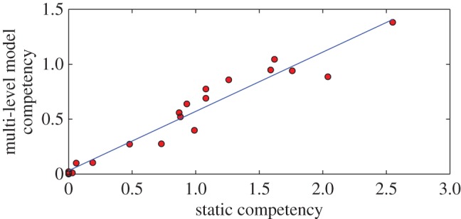
Correlation between multi-level model predicted competency and competency from Komar et al. [13] assuming static viraemia (r² = 0.94, slope = 0.54, p-value = 1×10⁻⁶). (Online version in colour.)

Komar et al. [13] assume that virus is constant over time (at a level equal to peak viraemia) and hence they overestimate the total amount of virus produced over the duration of infectivity. In reality, viraemia changes over time and is actual highest at the time of peak viraemia. Our estimates of competency account for this and hence are lower than those of Komar et al. [13]. Area under the curve in a simple model where virus increases linearly (on a log scale) and then declines linearly after some time forms a triangle. The triangle has approximately half the total area of the rectangle formed by assuming viraemia is maintained at peak levels throughout the duration of infection. Hence, our model has approximately half the area (and half the value) compared to the estimates of Komar et al. [13].

4.3. Scaling of biologically relevant quantities

A scaling relationship between a parameter η in our model and host body mass, M, is written as η∝M^α where α is the scaling exponent. Taking the logarithm of both sides of this relationship, we note

4.1

Thus, the scaling exponent can be derived as the slope of a log–log plot of η versus M.

In order to derive scaling relations with host body size, we used the slope of the correlation between individual-level averages of ODE parameters and species mass, when the correlation was statistically significant (figure 6, multi-level model). The scaling relationships and statistics are summarized in table 2. We observed that the production rate of infectious virions (p, PFU per day) is correlated and declines with species body mass (all species combined: p-value = 0.002, r² = 0.11, slope = −1.1; only passerines: p-value = 0.04, r² = 0.1, slope = −1). We note that although the 95% confidence interval (CI) for the slope [−1.5, 0.03] includes the theoretically predicted exponent of −0.25, the confidence interval is too large to provide a meaningful estimate of the scaling exponent.

Figure 6.

Scaling of biologically relevant quantities with host mass for the multi-level model: passerines (black square and black regression line, non-passerines (red circle and red regression line) and all combined (blue regression line). (a) Peak viraemia (V_p), slope =−0.82, p-value = 0.06, r² = 0.04. (b) WNV production rate (p), slope =−1.1, p-value = 0.002, r² = 0.11. (c) Inoculated density of virions (V₀), p-value = 0.35. (d) R₀, slope =−1.3, p-value = 0.006, r² = 0.09. (Online version in colour.)

Table 2.

Statistics of scaling relationships with species mass (all species combined) from multi-level model with target cell limitation (TCL) or an adaptive immune response (AIR).

parameters	combined slope	p	r2
p (TCL): WNV production rate	−1.1	0.002	0.11
p (AIR): WNV production rate	−0.84	0.04	0.05
R0 (TCL): basic reproductive number	−1.3	0.006	0.09
R0 (AIR): basic reproductive number	−0.57	0.08	0.04
p/δ (TCL): burst size	−1.1	0.001	0.12
p/δ (AIR): burst size	−0.86	0.03	0.06
Vp (TCL): peak viraemia	−0.82	0.06	0.04
Vp (AIR): peak viraemia	—	0.54	0.005
V0 (TCL): inoculated WNV density	—	0.35	0.1
V0 (AIR): inoculated WNV density	—	0.1	0.03
β (TCL): WNV infectivity	—	0.64	0.003
β (AIR): WNV infectivity	—	0.39	0.009
δ (TCL): death rate of productively infected cells	—	0.6	0.003
δ (AIR): death rate of productively infected cells	—	0.51	0.005
ρ (AIR): rate of adaptive immune system mediated virus neutralization	—	0.11	0.03
ti (AIR): time of initiation of IgM response	—	0.56	0.004

The basic reproductive number represents the average number of second-generation infections produced by a single infected cell placed in a population of susceptible cells. If R₀ is greater than 1, then an infection can be established, whereas an infection rapidly dies out if R₀ is less than 1. For the target cell limited model (equations (3.2)–(3.5)), R₀ is given by [47]

4.2

The basic reproductive number, R₀, had a significant overall decreasing correlation with mass (all species combined: p-value = 0.006, r² = 0.09, slope = − 1.3; only passerines: p-value = 7 × 10⁻⁵, r² = 0.33, slope = −3.7). Peak viraemia (P_v, the maximum viraemia attained by an individual over the time course of infection) had a marginally significant correlation with species mass (all species combined: p-value = 0.06, r² = 0.04, slope = −0.82).

The burst size (p/δ, PFU), representing the number of infectious virions released by an infected cell over its productively infected lifespan, had a significant decreasing relationship with species body mass (all species combined: p-value = 0.001, r² = 0.12, slope = −1.1; only passerines: p-value = 0.03, r² = 0.12, slope = −1.1). Also the viraemia at day 1 (V (1)) was correlated with mass (all species combined, p-value = 0.003, r² = 0.1, slope = −1.1).

The density of inoculated virions (V₀) and the infectivity of WNV (β) had no significant relationship with species mass (all species combined: p-value = 0.35, r² = 0.1 and p-value = 0.64, r² = 0.003). Finally, the death rate of productively infected cells (δ, d⁻¹) had no relationship with mass (all species combined, p = 0.6).

We also used the adaptive immune response model (equations (3.2)–(3.4), (3.6)–(3.7)) to investigate how parameters related to the immune response scale with host body mass (multi-level model, figure 7 and table 2). The rate of adaptive immune system mediated neutralization of virus (ρ, PRNT⁻¹₅₀ d⁻¹) did not have a significant relationship with body mass (all species combined: p-value = 0.11, r² = 0.03, slope = −0.19), although we observed that in passerines it declined significantly with mass (p-value = 0.04, r² = 0.1, slope = −0.51). The time of initiation of IgM response (t_i) also did not have a significant relationship with species mass (all species combined: slope = 0.002, p-value = 0.56, r² = 0.004; only passerines: slope = 0.01, p-value = 0.07, r² = 0.08).

Figure 7.

Scaling of immune response parameters with host mass for the multi-level model with immune response: passerines (black square) and non-passerines (red circle). (a) Rate of adaptive immune system mediated virus neutralization (ρ, PRNT⁻¹₅₀ d⁻¹). (b) Time of initiation of IgM response (t_i, days) (combined and each group separately are non-significant). (Online version in colour.)

The model parameter estimates and confidence intervals for all species are summarized in tables 3 and 4. The ODE model predictions for viraemia (for the parameters shown in tables 3 and 4) for all species are shown in figures 8–10.

Figure 9.

Predictions from the ODE model given by equations (3.2)–(3.5) for plasma virus concentration (in log₁₀ PFU ml⁻¹) over time post infection (blue) and experimental data on virus concentration (black). Parameters used are the mean for each species from the multi-level model. Data show the viraemia of the following species from [13]: (a–h) ring-billed gull, great-horned owl, American kestrel, killdeer, northern bobwhite, northern flicker, rock dove and American coot, respectively. (Online version in colour.)

Table 3.

Estimated parameters (mean and 95% CI) for all species from the multi-level model with target cell limitation (TCL). V₀, inoculated virus density (PFU ml⁻¹); β, rate constant of infection (ml d⁻¹); p, infectious virus production rate (PFU d⁻¹); δ, death rate of productively infected cells (d⁻¹).

species	V0	β	p	δ
fish crow	5 × 103 [4.3 × 103, 5.8 × 103]	3.7 × 10−9 [2.8 × 10−9, 4.8 × 10−9]	2.1 × 104 [1.8 × 104, 2.4 × 104]	4.8 [4.5, 5]
blue jay	2.9 × 103 [2.5 × 103, 3.3 × 103]	3.9 × 10−8 [3.3 × 10−8, 4.6 × 10−8]	4.9 × 104 [4.4 × 104, 5.5 × 104]	5.3 [4.9, 5.6]
American crow	740 [650.4, 842.2]	1.6 × 10−9 [1.4 × 10−9, 1.9 × 10−9]	1.4 × 104 [1.3 × 104, 1.6 × 104]	6.2 [5.9, 6.4]
common grackle	185.1 [163.1, 210]	4.4 × 10−8 [3.8 × 10−8, 5 × 10−8]	2.5 × 105 [2.2 × 105, 2.8 × 105]	6.8 [6.6, 7]
American robin	1.1 × 103 [0.9 × 103, 1.3 × 103]	4.8 × 10−8 [4.2 × 10−8, 5.4 × 10−8]	1.5 × 105 [1.3 × 105, 1.7 × 105]	7.4 [7.1, 7.6]
red-winged blackbird	731.4 [648.7, 824.6]	8 × 10−7 [7.2 × 10−7, 8.7 × 10−7]	1.5 × 104 [1.4 × 104, 1.6 × 104]	6.4 [6.2, 6.6]
black-billed magpie	1.4 × 103 [1.2 × 103, 1.5 × 103]	1 × 10−7 [0.9 × 10−7, 1.1 × 10−7]	5.2 × 104 [4.8 × 104, 5.7 × 104]	5.3 [5.1, 5.5]
house finch	305.9 [269.2, 347.8]	1.3 × 10−7 [1.1 × 10−7, 1.5 × 10−7]	3.5 × 104 [3.1 × 104, 3.8 × 104]	3.1 [2.9, 3.3]
house sparrow	3.4 × 103 [3 × 103, 3.9 × 103]	2.2 × 10−7 [1.9 × 10−7, 2.5 × 10−7]	7.4 × 104 [6.6 × 104, 8.2 × 104]	4.6 [4.5, 4.7]
mallard	164.2 [146.4, 184.1]	2.5 × 10−6 [2.3 × 10−6, 2.9 × 10−6]	3.3 × 103 [3 × 103, 3.7 × 103]	5.4 [5.2, 5.7]

Table 4.

Estimated parameters (mean and 95% CI) for all species from multi-level model with target cell limitation (TCL) (continued from table 3). V₀, inoculated virus density (PFU ml⁻¹); β, rate constant of infection (ml d⁻¹); p, infectious virus production rate (PFU d⁻¹); δ, death rate of productively infected cells (d⁻¹).

species	V0	β	p	δ
mourning dove	867.9 [750, 1000.4]	5.3 × 10−6 [4.8 × 10−6, 5.9 × 10−6]	1.1 × 103 [1 × 103, 1.2 × 103]	5.3 [5.1, 5.6]
ring-billed gull	3.2 × 103 [2.8 × 103, 3.7 × 103]	1.8 × 10−7 [1.6 × 10−7, 2.1 × 10−7]	2.8 × 104 [2.5 × 104, 3.1 × 104]	3.5 [3.4, 3.6]
great-horned owl	1 × 103 [0.9 × 103, 1.1 × 103]	3.4 × 10−7 [3.1 × 10−7, 3.7 × 10−7]	1.5 × 104 [1.4 × 104, 1.7 × 104]	4.6 [4.5, 4.9]
American kestrel	2.1 × 103 [1.8 × 103, 2.4 × 103]	2.5 × 10−7 [2.2 × 10−7, 2.9 × 10−7]	3.3 × 104 [3 × 104, 3.8 × 104]	5.5 [5.3, 5.7]
killdeer	871.7 [769.5, 987.3]	5.9 × 10−7 [5.3 × 10−7, 6.7 × 10−7]	1.9 × 104 [1.8 × 104, 2.1 × 104]	5.2 [4.9, 5.4]
northern bobwhite	4.7 × 103 [3.9 × 103, 5.6 × 103]	2.6 × 10−6 [2.1 × 10−6, 3.1 × 10−6]	1.1 × 103 [0.9 × 103, 1.3 × 103]	2.7 [2.5, 2.9]
northern flicker	250.3 [223.6, 280.2]	7.2 × 10−6 [6.6 × 10−6, 8 × 10−6]	884.3 [811.6, 963.5]	5.9 [5.7, 6.3]
rock dove	228.4 [200.7, 259.9]	8.5 × 10−5 [7.9 × 10−5, 9 × 10−5]	95.7 [90.8, 100.9]	5.5 [5.3, 5.7]
American coot	208.7 [182.4, 238.7]	2.1 × 10−5 [1.8 × 10−5, 2.3 × 10−5]	207.4 [187.9, 228.8]	5.3 [5, 5.6]
monk parakeet	2.3 × 103 [1.9 × 103, 2.7 × 103]	1.3 × 10−5 [1.1 × 10−5, 1.5 × 10−5]	296.3 [264.9, 331.5]	6.1 [5.7, 6.5]
budgerigar	674.7 [599.4, 759.4]	2.9 × 10−6 [2.5 × 10−6, 3.4 × 10−6]	860.8 [757.2, 978.6]	4.8 [4.5, 5.1]
Canada goose	647.3 [553.2, 757.3]	4.1 × 10−5 [3.7 × 10−5, 4.6 × 10−5]	144.5 [131, 159.4]	4.8 [4.5, 5.2]

We also show the posterior distributions of parameters for two selected species to highlight the differences in model parameters between these species in figure 11 (target cell limited model parameters V₀, β, p, δ for two species: American crows and Canadian geese). This underscores the variation in parameters between different species. Similar variation was seen between other species.

Figure 11.

(a–d) Posterior distribution of target cell limited model parameters for American crows. (e–h) Posterior distribution of target cell limited model parameters for Canadian geese. Parameters shown are V₀, inoculated virus density (PFU ml⁻¹); β, rate constant of infection (ml d⁻¹); p, infectious virus production rate (PFU d⁻¹); δ, death rate of productively infected cells (d⁻¹).

Finally, we show the trace plots of samples from the posterior distribution (the Monte Carlo Markov chain after burn-in and thinning) in figure 12. These show that the inference procedure converges around a particular value with variation around it. There is variation around a mean consistent with what would be observed when parameters have been identified. Similar behaviour was seen for posterior distributions of other species (data not shown).

Figure 12.

Trace of samples from the Monte Carlo Markov Chain after burn-in and thinning (taking every 5th sample). (a–d) Trace of target cell limited model parameters for American crows. (e–h) Trace of target cell limited model parameters for Canadian geese. Parameters shown are V₀, inoculated virus density (PFU ml⁻¹); β, rate constant of infection (ml d⁻¹); p, infectious virus production rate (PFU d⁻¹); δ, death rate of productively infected cells (d⁻¹). (Online version in colour.)

4.4. Accuracy in viraemia prediction

We estimated the accuracy of viraemia prediction by calculating three different estimates of a SSR between the data and the ODE model prediction (for both the multi-level and aggregated Bayesian models), as described in ‘Estimate of accuracy in viraemia prediction’ section.

We observed that the multi-level model produced more accurate estimates at the individual level and species level (figure 13a). A representative viraemia prediction for both the multi-level and aggregated model is also shown (figure 13b). The performance of both the models at the order level was similar.

Figure 13.

(a) Accuracy in viraemia prediction between multi-level model (blue) and aggregated model (red) for three different levels—individual, species and order. SSR—sum of squared residuals between model predicted viraemia and data. (b) A sample viraemia prediction from the multi-level (blue) and aggregated model (red).

We note that in some cases our hierarchical Bayesian models produce parameter estimates that appear to be biologically unreasonable, e.g. the production rate of WNV from infected cells (p) for some corvid species is predicted to be approximately 10⁸ PFU d⁻¹, which is unreasonably high. This could be due to the fact that the empirically measured viraemia goes up to 10¹⁵ PFU ml⁻¹ in some of these species and the initial susceptible cell population density (T₀ in our models) is much higher in corvids. This may suggest that other cell types are also available for infection in these species. Further experimental data on the susceptible cell population in corvid species may lead to more realistic estimates of the production rate (as these two parameters are correlated in our models).

5. Discussion

5.1. Summary

Understanding how quickly pathogens replicate and how quickly the immune system responds is important for predicting the epidemic spread of emerging pathogens. Host body size, through its correlation with metabolic rates, is theoretically predicted to impact pathogen replication and immune system response [9]. Prior work suggests that body mass affects pathogen replication [3,11,48], but immune response times are either independent of mass or increase only very slowly as mass increases [11,49]. Here, we use mathematical models of viral time courses from multiple species of birds infected by WNV to test more thoroughly how disease progression and immune response depend on host phylogeny and mass. The mathematical framework presented here is an approach to uncover systematic differences in disease progression and immune response in animals that differ in body mass and phylogeny.

Host phylogeny is an important determinant of the pathogenesis of WNV. Passerine species sustain more viraemia than non-passerine species, and corvid species are particularly susceptible to WNV infection [13]. Therefore, any analysis of disease dynamics in multi-host pathogens like WNV should take host phylogeny into account. We accomplish this using hierarchical Bayesian models that incorporate the hierarchical nature of phylogeny. We observe that the multi-level model produces more accurate predictions of viraemia at the individual and species level when compared with hierarchical models that have fewer levels of hierarchy (figure 13). Additionally, multi-level models with passerines and non-passerines or just passerines (figure 4a–d) produced more realistic and more strongly peaked distributions of R₀ and burst size, than a multi-level model with only corvids (figure 4e,f) and the aggregated model (figure 14). This appears to be due to the ability of multi-level models to pool information at the species level from different related species.

A major contribution of this work is a computational framework for infectious within-host disease modelling that leverages data from multiple species. This is particularly important given recent analysis of many zoonotic diseases that can or have the potential to cross species boundaries and infect humans [50]. Our models estimate a competency for infected hosts to infect mosquito vectors that can then sustain the disease between hosts. This link between within- and between-host disease models is an important step towards understanding the threat from emerging zoonotic diseases and identifying likely candidate species for biosurveillance.

5.2. Effect of host phylogeny on within-host pathogen replication

We quantified the basic reproductive number (R₀), which represents the average number of infections produced by a single infected cell. The mean values of R₀ from the multi-level model are higher for passerine species (R₀ = 23.8) compared to non-passerines (R₀ = 4.7) (figure 4a,b). Within passerines, corvid species have the highest mean value of R₀ = 93.2.

Burst sizes of passerine species (8690 PFU) are also much higher than those in non-passerines (340 PFU) (figure 4a,b). This is consistent with experimental studies that found passerines and corvids have higher reservoir competency (ability to transmit infection to mosquitoes) than non-passerines [13]. Overall, host phylogeny emerges as a key determinant of biologically relevant quantities like the basic reproductive number and burst size. The mean passerine values for R₀ (23.8) and burst size (8690 PFU) are also higher than the corresponding model's predicted values in mice (mean R₀ = 2.5 and burst size = 3 PFU [37]).

We also calculated a reservoir competence index that indicates the relative number of infectious mosquitoes that would be derived from feeding on these hosts (§3.6) and accounts for time-varying viraemia and species relatedness (via the multi-level Bayesian model). The mean reservoir competence for passerine species (0.8) is higher than that of non-passerines (0.2). This lends mechanistic insight into why some species (smaller passerine species) are pathogen reservoirs and some (larger non-passerine species) are potentially dead-end hosts for WNV.

5.3. Effect of host body size on virion production rate and immune response

Individual cellular metabolic rates and biological times, if constrained by host metabolism, are expected to scale with host body mass as M^−1/4 and M^1/4, respectively [4–9]. We observe that the production rate of infectious virions (p) declined significantly with host body mass. While the 95% confidence interval for the slope (CI = [−1.5, 0.03]) includes the theoretically predicted exponent of −0.25 (figure 6), the confidence interval is too large to provide a meaningful estimate of the scaling exponent.

The death rate of productively infected cells (δ), also theoretically predicted to decrease with mass, had no relationship with species mass. The basic reproductive number (R₀) declined significantly with body mass (figure 6) and the relationship is even more significant within passerine species. This is most likely because the production rate of virions (p), a component of the R₀ (equation (4.2)), declined with mass.

We found that the mean of peak viral concentration in serum (peak viraemia) declines with species body mass (figure 6) although the correlation was only marginally significant. Additionally, most passerine species had higher peak viraemia than non-passerines. This is likely because most of the passerine species had a higher value of the viral production rate (p) than the non-passerines. Overall, we observed modest trends in the direction predicted by scaling theory, but host phylogeny is a more important predictor of WNV dynamics.

The density of inoculated virions (V₀) has no significant relationship with species mass (figure 6). This is surprising because if mosquitoes inoculated a fixed dose directly into the host bloodstream, the density of virions (V₀) would be expected to decline with host mass because the dilution would be higher in the larger blood volume of a larger species. Mosquito-inoculated WNV, that is initially localized at the site of infection [51], is taken up by immune cells to nearby lymph nodes and then trafficks to different organs via the bloodstream. However, for computational efficiency, we use differential equation models that assume all components are well mixed. Our results point to the importance of accounting for spatial patterns of viral spread, especially in the initial stages of an infection when virus is localized, and this should be considered in future work.

The target cell limited and adaptive immune response models both produce similar scaling predictions when coupled to the multi-level hierarchical model (table 2).

We used the adaptive immune response model (equations (3.2)–(3.4), (3.6)–(3.7)) to investigate how parameters related to the immune response scale with host body mass (multi-level model, figure 7). The rate at which the adaptive (antibody) immune response neutralizes virus (ρ) did not have a significant relationship with body mass, although we observed that in passerine species it declined significantly with mass. The time of initiation of the adaptive (antibody) immune response (t_i) also did not have a significant relationship with species mass.

Hence, in sharp contrast to the vast majority of biological rates that slow systematically as the body size increases [7,8], the rate at which the adaptive (antibody) immune response clears WNV and the time at which it is initiated do not vary systematically with mass (figure 7). Previous work has suggested two plausible mechanisms that both enable this scale-invariant search and response. A sub-modular architecture of lymph nodes, which balances local pathogen detection and global antibody production, may lead to nearly scale-invariant search and response times [11,52]. Chemical signals released from infected sites also help guide immune system cells towards infected regions, reducing the time for the immune system to search for infection [12,53,54].

5.4. Implications for spread of West Nile Virus and other zoonotic diseases

Our modelling suggests that rates of WNV production decline with species mass, whereas rates and times related to the adaptive immune response do not vary systematically with mass. Taken together, these results provide an understanding of how epidemiological determinants vary with species body mass. The probability of infecting an uninfected mosquito increases with viraemia above a certain threshold for WNV [13]. This has also been observed for other flaviviruses such as dengue virus [55,56]). Above a threshold of viraemia of 10⁵ PFU ml⁻¹ of blood, a host is capable of infecting an uninfected mosquito and maintaining WNV in an enzootic cycle [13]. Hence, hosts that can sustain high viraemia above this threshold and for a longer duration are pathogen reservoirs [13]. The dependence of viraemia on host mass and phylogeny may give important insights into the role of mass and phylogeny on the spread of WNV. For example, larger non-passerine species, predicted to have lower viraemia, may be less competent as pathogen reservoirs.

Incorporating our within-host viral dynamics model into a between-host model that incorporates interactions between vectors and hosts, mosquito biting preferences [57–59] and bird abundance would be a fruitful avenue for future work. This analysis should consider the multiple ways in which host body size and phylogeny effect mosquito biting rates. Larger animals might have a greater probability of receiving an infective bite due to their larger surface area. However, the relationship between body size and the frequency of mosquito bites is complicated by several factors. For example, mosquitoes also have distinct biting preferences across species [57,58] and the ecological niche occupied by the species may influence biting rates. The effect of total body surface area may be limited given that the footpads, neck and the face are the only exposed regions in birds that do not have feathers and are most accessible for biting. Finally, body size affects population density which is approximately inversely proportional to host metabolism [60], and relative abundance of a species is another important factor in determining the spread of WNV. There are many unknowns and we speculate that models that combine species body size and other ecological factors with within-host modelling will be important in predicting outcomes of emerging diseases and formulating outbreak control strategies, as has been proposed for vector-borne diseases [61], dengue virus [55], Zika virus [62] and Ebola virus [63].

Our analysis suggests an important role for both species mass and host phylogeny in dictating epidemiological determinants such as the basic reproductive number, WNV production rate, peak viraemia in blood and host competency to infect mosquitoes. Our model is based on a principled analysis and gives a quantitative prediction for key epidemiological determinants and how they vary with species mass and phylogeny. The WNV production rate (p) and the basic reproductive number (R₀) decline with host body mass (figure 6). The relationship is even more significant within passerine species (figure 6).

We calculated a reservoir competence index that indicates the relative number of infectious mosquitoes that would be derived from feeding on these hosts (§3.6). Our reservoir competency index is a refinement on previously published indices [13] because they take time-varying viraemia and species relatedness (via the multi-level Bayesian model) into account. The reservoir competency indices we calculate are correlated with and approximately half of the estimates in Komar et al. [13] (figure 5). The mean reservoir competence for passerine species (0.8) is higher than that of non-passerines (0.2). Thus, our models provide insight into why some species (smaller passerine species) are pathogen reservoirs and some (larger non-passerine species) are potentially dead-end hosts for WNV.

WNV infection progresses along multiple scales: infection within hosts is related to dynamics of WNV spread between hosts by mosquito vectors. Coupling two different processes over multiple scales, from individual cells to epidemic spread in bird populations, is challenging and could yield valuable insights. Our predictions of host competency to infect mosquitoes (equation (3.8) and figure 5) can be coupled to models of WNV spread between multiple species. Such an approach would help link within-host WNV dynamics to dynamics between hosts and may help produce accurate estimates of spread of WNV.

Hierarchical Bayesian models coupled with within-host viral dynamics models can leverage data from multiple species to infer how body size and host phylogeny affect viral dynamics. This approach can be applied to model other zoonotic diseases and multi-host pathogens [37], particularly other emerging viruses such as dengue [64,52], Ebola [63] and Zika virus [33,34,62].

Data accessibility

This article has no additional data.

Author's contributions

S.B. carried out the analysis and implementation, participated in the design of the study and drafted the manuscript; A.S.P. carried out the analysis, drafted the manuscript and coordinated the study. M.M. carried out the analysis, drafted the manuscript and coordinated the study. All authors gave final approval for publication.

Competing interests

We declare we have no competing interests.

Funding

M.M. acknowledges the support from a James S. McDonnell Foundation Complex Systems Scholar Award and National Science Foundation EF 1038682. Portions of this work were performed under the auspices of the US Department of Energy under contract DE-AC52-06NA25396 and supported by NIH grants R01-AI078881, R01-OD011095, R01-AI028433 and HHSN272201000055C to A.S.P. The authors acknowledge the UNM Center for Evolutionary and Theoretical Immunology (CETI) funded by the NIH IDeA Program of the National Center for Research Resources P20RR018754 for funding and support of this collaboration.

References

- 1.Grace D, et al. 2012. Mapping of poverty and likely zoonoses hotspots. Report to the department for international development.
- 2.Woolhouse M, Taylor L, Haydon D. 2001. Population biology of multihost pathogens. Science 292, 1109–1112. ( 10.1126/science.1059026) [DOI] [PubMed] [Google Scholar]
- 3.Cable J, Enquist B, Moses M. 2007. The allometry of host–pathogen interactions. PLoS ONE 2, e1130 ( 10.1371/journal.pone.0001130) [DOI] [PMC free article] [PubMed] [Google Scholar]
- 4.Kleiber M. 1947. Body size and metabolic rate. Physiol. Rev. 27, 511–541. [DOI] [PubMed] [Google Scholar]
- 5.Kleiber M. 1932. Body size and metabolism. Hilgardia: J. Agric. Sci. 6, 315–353. ( 10.3733/hilg.v06n11p315) [DOI] [Google Scholar]
- 6.Peters RH. 1986. The ecological implications of body size, vol. 2 Cambridge, UK: Cambridge University Press. [Google Scholar]
- 7.West G, Brown J, Enquist B. 1997. A general model for the origin of allometric scaling laws in biology. Science 276, 122–126. ( 10.1126/science.276.5309.122) [DOI] [PubMed] [Google Scholar]
- 8.Brown JH, Gillooly JF, Allen AP, Savage VM, West GB. 2004. Toward a metabolic theory of ecology. Ecology 85, 1771–1789. ( 10.1890/03-9000) [DOI] [Google Scholar]
- 9.Wiegel FW, Perelson A. 2004. Some scaling principles for the immune system. Immunol. Cell Biol. 82, 127–131. ( 10.1046/j.0818-9641.2004.01229.x) [DOI] [PubMed] [Google Scholar]
- 10.Althaus CL. 2015. Of mice, macaques and men: scaling of virus dynamics and immune responses. Front. Microbiol. 6, 355 ( 10.3389/fmicb.2015.00355) [DOI] [PMC free article] [PubMed] [Google Scholar]
- 11.Banerjee S, Moses M. 2010. Scale invariance of immune system response rates and times: perspectives on immune system architecture and implications for artificial immune systems. Swarm Intell. 4, 301–318. ( 10.1007/s11721-010-0048-2) [DOI] [Google Scholar]
- 12.Banerjee S, Levin D, Koster F, Forrest S, Moses M. 2011. The value of inflammatory signals in adaptive immune responses. In Artificial Immune Systems, 10th International Conference, ICARIS 2011 (eds Liò P, Nicosia G, Stibor T). Lecture Notes in Computer Science, vol. 6825, pp. 1–14. Berlin, Germany: Springer. [Google Scholar]
- 13.Komar N, Langevin S, Hinten S, Nemeth N, Edwards E, Hettler DL, Davis BS, Bowen RA, Bunning ML. 2003. Experimental infection of North American birds with the New York 1999 strain of West Nile virus. Emerg. Infect. Dis. 9, 311–322. ( 10.3201/eid0903.020628) [DOI] [PMC free article] [PubMed] [Google Scholar]
- 14.Rouder J, Lu J, Speckman P. 2005. A hierarchical model for estimating response time distributions. Psychon. Bull. Rev. 12, 195–223. ( 10.3758/BF03257252) [DOI] [PubMed] [Google Scholar]
- 15.Pearl J. 2009. Causality. Cambridge, UK: Cambridge University Press. [Google Scholar]
- 16.Fei-Fei L, Perona P. 2005. A bayesian hierarchical model for learning natural scene categories. In Proceedings of the 2005 IEEE Computer Society Conference on Computer Vision and Pattern Recognition (CVPR'05), vol. 2, pp. 524–531. Washington, DC: IEEE Computer Society. [Google Scholar]
- 17.Wikle C. 2003. Hierarchical bayesian models for predicting the spread of ecological processes. Ecology 84, 1382–1394. ( 10.1890/0012-9658(2003)084%5B1382:HBMFPT%5D2.0.CO;2) [DOI] [Google Scholar]
- 18.Wikle C, Berliner L, Cressie N. 1998. Hierarchical bayesian space-time models. Environ. Ecol. Stat. 5, 117–154. ( 10.1023/A:1009662704779) [DOI] [Google Scholar]
- 19.Huang Y, Wu H, Acosta EP. 2010. Hierarchical Bayesian inference for HIV dynamic differential equation models incorporating multiple treatment factors. Biometrical J. 52, 470–486. ( 10.1002/bimj.200900173) [DOI] [PMC free article] [PubMed] [Google Scholar]
- 20.Huang Y, Liu D, Wu H. 2006. Hierarchical Bayesian methods for estimation of parameters in a longitudinal HIV dynamic system. Biometrics 62, 413–423. ( 10.1111/j.1541-0420.2005.00447.x) [DOI] [PMC free article] [PubMed] [Google Scholar]
- 21.Han C, Chaloner K, Perelson A. 2002. Bayesian analysis of a population HIV dynamic model. Case studies in Bayesian Statistics, vol. 6 (eds C Gatsonis, RE Kass, A Carriquiry, A Gelman, D Higdon, DK Parker, I Vardinelli) Lecture Notes in Statistics, pp. 223–237. New York, NY: Springer. [Google Scholar]
- 22.Canini L, Carrat F. 2011. Population modeling of influenza A/H1N1 virus kinetics and symptom dynamics. J. Virol. 85, 2764–2770. ( 10.1128/JVI.01318-10) [DOI] [PMC free article] [PubMed] [Google Scholar]
- 23.Hayes EB, Komar N, Nasci RS, Montgomery SP, O'Leary DR, Campbell GL. 2005. Epidemiology and transmission dynamics of West Nile virus disease. Emerg. Infect. Dis. 11, 1167–1173. ( 10.3201/eid1108.050289a) [DOI] [PMC free article] [PubMed] [Google Scholar]
- 24.Deardorff E, et al. 2006. Introductions of West Nile virus strains to Mexico. Emerg. Infect. Dis. 12, 314–318. ( 10.3201/eid1202.050871) [DOI] [PMC free article] [PubMed] [Google Scholar]
- 25.Komar N, Clark GG. 2006. West Nile virus activity in Latin America and the Caribbean. Rev. Panam Salud Publica 19, 112–117. ( 10.1590/S1020-49892006000200006) [DOI] [PubMed] [Google Scholar]
- 26.Lanciotti RS, et al. 1999. Origin of the West Nile virus responsible for an outbreak of encephalitis in the northeastern United States. Science 286, 2333–2337. ( 10.1126/science.286.5448.2333) [DOI] [PubMed] [Google Scholar]
- 27.Samuel MA, Diamond MS. 2006. Pathogenesis of West Nile virus infection: a balance between virulence, innate and adaptive immunity, and viral evasion. J. Virol. 80, 9349–9360. ( 10.1128/JVI.01122-06) [DOI] [PMC free article] [PubMed] [Google Scholar]
- 28.Stafford M, Cao Y, Ho D, Corey L. 2000. Modeling plasma virus concentration and CD4+ T cell kinetics during primary HIV infection. J. Theor. Biol. 203, 285–301. ( 10.1006/jtbi.2000.1076) [DOI] [PubMed] [Google Scholar]
- 29.Baccam P, Beauchemin C, Macken C, Hayden F, Perelson A. 2006. Kinetics of influenza a virus infection in humans. J. Virol. 80, 7590–7599. ( 10.1128/JVI.01623-05) [DOI] [PMC free article] [PubMed] [Google Scholar]
- 30.Rong L, Dahari H, Ribeiro RM, Perelson AS. 2010. Rapid emergence of protease inhibitor resistance in hepatitis C virus. Sci. Transl. Med. 2, 30ra32 ( 10.1126/scitranslmed.3000544) [DOI] [PMC free article] [PubMed] [Google Scholar]
- 31.Vaidya NK, Ribeiro RM, Miller CJ, Perelson AS. 2010. Viral dynamics during primary simian immunodeficiency virus infection: effect of time-dependent virus infectivity. J. Virol. 84, 4302–4310. ( 10.1128/JVI.02284-09) [DOI] [PMC free article] [PubMed] [Google Scholar]
- 32.Nowak MA, Bonhoeffer S, Hill AM, Boehme R, Thomas HC, McDade H. 1996. Viral dynamics in hepatitis B virus infection. Proc. Natl Acad. Sci. USA 93, 4398–4402. ( 10.1073/pnas.93.9.4398) [DOI] [PMC free article] [PubMed] [Google Scholar]
- 33.Osuna CE, et al. 2016. Zika viral dynamics and shedding in rhesus and cynomolgus macaques. Nat. Med. 22, 1448–1455. ( 10.1038/nm.4206) [DOI] [PMC free article] [PubMed] [Google Scholar]
- 34.Best K, Guedj J, Madelain V, de Lamballerie X, Lim SY, Osuna CE, Whitney JB, Perelson AS. 2017. Zika plasma viral dynamics in nonhuman primates provides insights into early infection and antiviral strategies. Proc. Natl Acad. Sci. USA 114, 8847–8852. ( 10.1073/pnas.1704011114) [DOI] [PMC free article] [PubMed] [Google Scholar]
- 35.Diamond MS, Sitati EM, Friend LD, Higgs S, Shrestha B, Engle M. 2003. A critical role for induced IgM in the protection against West Nile virus infection. J. Exp. Med. 198, 1853–1862. ( 10.1084/jem.20031223) [DOI] [PMC free article] [PubMed] [Google Scholar]
- 36.Diamond MS, Shrestha B, Marri A, Mahan D, Engle M. 2003. B cells and antibody play critical roles in the immediate defense of disseminated infection by West Nile encephalitis virus. J. Virol. 77, 2578–2586. ( 10.1128/JVI.77.4.2578-2586.2003) [DOI] [PMC free article] [PubMed] [Google Scholar]
- 37.Banerjee S, Guedj J, Ribeiro RM, Moses M, Perelson AS. 2016. Estimating biologically relevant parameters under uncertainty for experimental within-host murine West Nile virus infection. J. R. Soc. Interface 13, 20160130 ( 10.1098/rsif.2016.0130) [DOI] [PMC free article] [PubMed] [Google Scholar]
- 38.The MathWorks Inc. 2011. MATLAB version 7.13.0.564.
- 39.Styer LM, Kent KA, Albright RG, Bennett CJ, Kramer LD, Bernard KA. 2007. Mosquitoes inoculate high doses of West Nile virus as they probe and feed on live hosts. PLoS Pathog. 3, e132 ( 10.1371/journal.ppat.0030132) [DOI] [PMC free article] [PubMed] [Google Scholar]
- 40.Martín P, Ruiz SR, Martínez del Hoyo G, Anjuère F, Vargas HH, López-Bravo M, Ardavín C. 2002. Dramatic increase in lymph node dendritic cell number during infection by the mouse mammary tumor virus occurs by a CD62L-dependent blood-borne DC recruitment. Blood 99, 1282–1288. ( 10.1182/blood.V99.4.1282) [DOI] [PubMed] [Google Scholar]
- 41.Purtha W, Chachu K, Virgin H, Diamond MS. 2008. Early B-cell activation after West Nile virus infection requires alpha/beta interferon but not antigen receptor signaling. J. Virol. 82, 10 964–10 974. ( 10.1128/JVI.01646-08) [DOI] [PMC free article] [PubMed] [Google Scholar]
- 42.Cheeran MCJ, Hu S, Sheng WS, Rashid A, Peterson PK, Lokensgard JR. 2005. Differential responses of human brain cells to West Nile virus infection. J. Neurovirol. 11, 512–524. ( 10.1080/13550280500384982) [DOI] [PubMed] [Google Scholar]
- 43.Clapham HE, Tricou V, Van Vinh Chau N, Simmons CP, Ferguson NM. 2014. Within-host viral dynamics of dengue serotype 1 infection. J. R. Soc. Interface 11, 20140094 ( 10.1098/rsif.2014.0094) [DOI] [PMC free article] [PubMed] [Google Scholar]
- 44.Carlin B, Louis T. 1997. Bayes and empirical bayes methods for data analysis. Stat. Comput. 7, 153–154. ( 10.1023/A:1018577817064) [DOI] [Google Scholar]
- 45.Gilks W, Richardson S, Spiegelhalter D. 1995. Markov Chain Monte Carlo in practice: interdisciplinary statistics, vol. 2 London, UK: Chapman & Hall/CRC. [Google Scholar]
- 46.Gelfand A, Smith A. 1990. Sampling-based approaches to calculating marginal densities. J. Am. Stat. Assoc. 85, 398–409. ( 10.1080/01621459.1990.10476213) [DOI] [Google Scholar]
- 47.Nowak M, May RM. 2000. Virus dynamics: mathematical principles of immunology and virology. Oxford, UK: Oxford University Press. [Google Scholar]
- 48.Banerjee S, Moses M. 2009. A hybrid agent based and differential equation model of body size effects on pathogen replication and immune system response. In Artificial Immune Systems, 8th International Conference, ICARIS 2009 (eds Andrews PS, Timmis J, Owens NDL, Aickelin U, Hart E, Hone A, Tyrrell AM). Lecture Notes in Computer Science, vol. 5666, pp. 14–18. Berlin, Germany: Springer. [Google Scholar]
- 49.Moses M, Banerjee S. 2011. Biologically inspired design principles for scalable, robust, adaptive, decentralized search and automated response (RADAR). In Proc. of the 2011 IEEE Conference on Artificial Life, pp. 30–37. Washington, DC: IEEE Computer Society. [Google Scholar]
- 50.Olival KJ, Hosseini PR, Zambrana-Torrelio C, Ross N, Bogich TL, Daszak P. 2017. Host and viral traits predict zoonotic spillover from mammals. Nature 546, 646–650. ( 10.1038/nature22975) [DOI] [PMC free article] [PubMed] [Google Scholar]
- 51.Styer LM, Kent KA, Albright RG, Bennett CJ, Kramer LD, Bernard KA. 2007. Mosquitoes inoculate high doses of West Nile virus as they probe and feed on live hosts. PLoS Pathog. 3, 1262–1270. ( 10.1371/journal.ppat.0030132) [DOI] [PMC free article] [PubMed] [Google Scholar]
- 52.Banerjee S. 2013. Scaling in the immune system. PhD thesis, University of New Mexico, USA. [Google Scholar]
- 53.Banerjee S, Moses M. 2009. A hybrid agent based and differential equation model of body size effects on pathogen replication and immune system response. In Lecture notes in computer science, vol. 5666 Artificial immune systems, 8th international conference, ICARIS 2009 (eds Andrews PS, et al.), pp. 14–18. Berlin, Germany: Springer. [Google Scholar]
- 54.Banerjee S, Moses M. 2010. Modular RADAR: an immune system inspired search and response strategy for distributed systems. In Lecture notes in computer science, vol. 6209 Artificial immune systems, 9th international conference, ICARIS 2010 (eds Hart E, et al.), pp. 116–129. Berlin, Germany: Springer. [Google Scholar]
- 55.Clapham HE. 2013. Modelling dengue infection dynamics and the impact of control measures. Ph.D. thesis, Imperial College London.
- 56.MinhNguyen N, et al. 2013. Host and viral features of human dengue cases shape the population of infected and infectious Aedes aegypti mosquitoes. Proc. Natl Acad. Sci. USA 110, 9072–9077. ( 10.1073/pnas.1303395110) [DOI] [PMC free article] [PubMed] [Google Scholar]
- 57.Hassan HK, Cupp EW, Hill GE, Katholi CR, Klingler K, Unnasch TR. 2003. Avian host preference by vectors of eastern equine encephalomyelitis virus. Am. J. Trop. Med. Hyg. 69, 641–647. [PubMed] [Google Scholar]
- 58.Kilpatrick AM, Kramer LD, Jones MJ, Marra PP, Daszak P. 2006. West Nile virus epidemics in North America are driven by shifts in mosquito feeding behavior. PLoS Biol. 4, 606–610. ( 10.1371/journal.pbio.0040082) [DOI] [PMC free article] [PubMed] [Google Scholar]
- 59.Farajollahi A, Fonseca DM, Kramer LD, Marm Kilpatrick A. 2011. ‘Bird biting’ mosquitoes and human disease: a review of the role of Culex pipiens complex mosquitoes in epidemiology. Infect. Genet. Evol. 11, 1577–1585. ( 10.1016/j.meegid.2011.08.013) [DOI] [PMC free article] [PubMed] [Google Scholar]
- 60.Damuth J. 1981. Population density and body size in mammals. Nature 290, 699–700. ( 10.1038/290699a0) [DOI] [Google Scholar]
- 61.Dobson A. 2004. Population dynamics of pathogens with multiple host species. Am. Nat. 164, 64–78. ( 10.1086/424681) [DOI] [PubMed] [Google Scholar]
- 62.Ferguson NM, Cucunubá ZM, Dorigatti I, Nedjati-Gilani GL, Donnelly CA, Basáñez MG, Nouvellet P, Lessler J. 2016. Countering the Zika epidemic in Latin America. Science 353, 353–354. ( 10.1126/science.aag0219) [DOI] [PMC free article] [PubMed] [Google Scholar]
- 63.Castillo-Chavez C, Curtiss R, Daszak P, Levin SA, Patterson-Lomba O, Perrings C, Poste G, Towers S. 2015. Beyond Ebola: lessons to mitigate future pandemics. Lancet Global Health 3, e354–e355. ( 10.1016/S2214-109X(15)00068-6) [DOI] [PMC free article] [PubMed] [Google Scholar]
- 64.Clapham HE, Quyen TH, Kien DTH, Dorigatti I, Simmons CP, Ferguson NM. 2016. Modelling virus and antibody dynamics during dengue virus infection suggests a role for antibody in virus clearance. PLoS Comput. Biol. 12, e1004951 ( 10.1371/journal.pcbi.1004951) [DOI] [PMC free article] [PubMed] [Google Scholar]
Associated Data
This section collects any data citations, data availability statements, or supplementary materials included in this article.
Supplementary Materials
Data Availability Statement