Semiparametric regression analysis for alternating recurrent event data

Abstract

Alternating recurrent event data arise frequently in clinical and epidemiologic studies, where two types of events such as hospital admission and discharge occur alternately over time. The two alternating states defined by these recurrent events could each carry important and distinct information about a patient’s underlying health condition and/or the quality of care. In this paper, we propose a semiparametric method for evaluating covariate effects on the two alternating states jointly. The proposed methodology accounts for the dependence among the alternating states as well as the heterogeneity across patients via a frailty with unspecified distribution. Moreover, the estimation procedure, which is based on smooth estimating equations, not only properly addresses challenges such as induced dependent censoring and intercept sampling bias commonly confronted in serial event gap time data, but also is more computationally tractable than the existing rank-based methods. The proposed methods are evaluated by simulation studies and illustrated by analyzing psychiatric contacts from the South Verona Psychiatric Case Register.

1. Introduction

Recurrent event data analysis focuses on modeling and estimation of the risk of event occurrence over time and has a wide range of applications in a variety of fields including in reliability, medicine, social sciences, economics, and criminology. In many applications, the study endpoints can be characterized by two different alternating events. For example, patients with chronic diseases may be repeatedly admitted to and discharged from hospital, thus creating an alternating sequence of care periods and break periods. In studies of depression, participants may cycle back and forth between periods of normal mood and depressive episodes. Another important example is the relapse phase and the remission phase of a reversible disease, where patients may alternate between the two disease states. Such data structure is referred to as alternating recurrent event data in this paper to distinguish from its univariate counterpart where all recurrent events are of the same type. It is important to point out that the duration of the two types of time periods can each carry distinct information about the underlying health condition of patients and/or the quality of care. For example, a shorter hospital stay can indicate better treatment effect or quality of care, while a short break period would suggest ineffective maintenance strategies in chronically ill patients. Therefore, it is of interest to develop efficient statistical methods that can make full use of the observed data to evaluate the effects of treatment and risk factors on the two alternating states.

When the gap time, that is, the duration between consecutive events, is the outcome of interest, it is known that the sequential structure of recurrent events generates analytical challenges [1, 2]. For example, because the observable region of the jth gap time (j ≥ 2) is given by the difference between the overall censoring time and the j − 1th event time, the second and higher order gap times are subject to induced dependent censoring as recurrent gap times of the same subject are usually correlated. This is the case even when the overall censoring time is independent of the recurrent event process. In addition, because longer gap times are more likely to be censored, the last censored gap times tend to be longer than the observed uncensored gap times; the phenomenon is known as length bias due to intercept sampling. Finally, the number of gap times is informative about the underlying recurrent event process, as high-risk patients tend to have shorter times between consecutive events, thus more gap times. In the literature, various statistical methods have been developed for analyzing gap time data in the setting of univariate recurrent events. In particular, some authors considered nonparametric estimation of the gap time distribution [1, 3, 4], while others have studied various semiparametric regression models for evaluating covariate effects on the gap times [5, 6, 7, 8, 9, 10, 11, 12, 13, 14]. Note that the aforementioned methodologies for univariate recurrent events are not directly applicable to analyzing the pooled gap times between alternating recurrent events, as the two states of an alternating recurrent event process usually have distinct biological meanings and hence different distributions. It is also not appropriate, as discussed in [15], to apply these models to the two different types of gap times separately due to the induced dependent censoring. It is theoretically justifiable to apply these methods to the sum of the two states; for example, one may consider the elapse times from one hospital admission to the next hospital admission of a patient by ignoring the information about the time of discharge. This simplified approach, however, can not determine if the covariates are associated with the length of the care periods or the break periods, or both, and thus the rich information available from the alternating recurrent gap time data is not fully utilized. In fact, a treatment that shortens the care periods and at the same time prolongs the break periods could be deemed as ineffective if the treatment effect is evaluated based on the elapse times between hospital admission times using univariate recurrent gap time methods.

The development of statistical methods for alternating recurrent event data has been scarce. Huang and Wang [2] considered nonparametric estimation of the joint distribution of the two alternating states. While nonparametric estimation can serve as a basis for exploring the underlying recurrent event process, regression methods would be more attractive to researchers who are interested in identifying risk factors that are related to the duration of each state. In an early work by Xue and Brookmeyer [16], a semiparametric bivariate frailty model was proposed for the two types of gap times, where a parametric assumption for the joint distribution of the frailties is imposed for deriving maximum likelihood estimator. More recently, Yan and Fine [15] proposed a temporal process regression method focusing on the frequency and the cumulative length of one of the two alternating states. Chang [6] considered accelerated failure time (AFT) models for both types of alternating gap times and employed a rank-based estimating equation approach for model estimation. However, the rank-based estimating equation approach for AFT models is seldom used in applications due to the lack of efficient and reliable computational methods for obtaining parameter estimates and the corresponding variance estimates [17, 18]. The main difficulty in the implementation of rank-based estimation procedure lies in the nonsmoothness of the estimating functions. Unfortunately, the same argument applies to the estimation procedure proposed by Chang [6], making it less attractive for practical use.

In this paper, we propose a semiparametric estimation approach under the AFT model. We adapt the multi-state model studied by Huang [19] to the first pair of gap times from alternating recurrent gap time data and extend it to include the recurrent pairs using a within-subject averaging technique [11]. The proposed methodology is based on U-statistics that are continuous and compactly differentiable, and as a result, is expected to be more computationally tractable than that proposed by Chang [6]. The remainder of the article is organized as follows. In Section 2, we introduce the data structure and assumptions of the proposed model. In Section 3, we briefly review the estimation method developed by Huang [19] for multi-state data and introduce our proposed method for alternating recurrent events with large sample properties being established. In Section 4, we conduct a series of simulation studies to demonstrate the performance of the proposed method and compare it with the rank-based estimation procedures proposed by Chang [6]. Application of our proposed method to a psychiatric case register (PCR) data is presented in Section 5. Some concluding remarks can be found in Section 6.

2. The Model

To facilitate our discussion, we take the alternating sequence of care and break periods in hospitalization data as an example. Suppose that a group of patients are recruited to a study when they are admitted to a hospital due to a certain disease and followed up on any recurrent hospitalizations due to the same disease until the end of the study. In the absence of censoring, we denote the duration of the care and break periods due to the jth hospitalization episode of subject i as $X_{ij}^0$ and $Y_{ij}^0$, respectively, then the recurrent hospitalization process of subject i’s can be denoted by $N_i=\left\{\left(X_{i1}^0,Y_{i1}^0\right),\left(X_{i2}^0,Y_{i2}^0\right),\dots \right\}$,i=1,…,n. Let a p × 1 vector A_i denote the baseline covariates and γ_i = (γ_i1, γ_i2)^⊤ a subject-specific latent vector. We assume that conditioning on A_i and γ_i, the bivariate pairs $\left(X_{ij}^0,Y_{ij}^0\right)$, j=1,2,…, are independently and identically distributed (i.i.d.) within subject i. Thus, the pairs of durations of the care and break periods can be viewed as an alternating renewal process [20] given the baseline covariates and the latent random vector.

To assess the association between covariates and the lengths of care and break periods, we assume that each period is linearly related to covariates in the logarithmic scale:

$$\log X_{ij}^0={\gamma }_{i1}+{\mathbf{A}}_i^{\top }{\mathit{\beta }}_1+{\epsilon }_{ij1,}$$ (1)

$$\log Y_{ij}^0={\gamma }_{i2}+{\mathbf{A}}_i^{\top }{\mathit{\beta }}_2+{\epsilon }_{ij2,}$$ (2)

where β₁ and β₂ are the regression coefficients for the care and break periods, respectively; and ε_ijk, i = 1,…, n, j = 1, 2,…, and k = 1, 2, are mutually independent random errors with mean zero. The distributions of γ_i and ε_ijk are left unspecified. The latent vector γ_i characterizes the correlation among the gap times within a subject. Specifically, the association between $X_{ij}^0$ and $Y_{ij}^0$ is characterized by the correlation of γ_i1 and γ_i2, whereas the variances of γ_i1 and γ_i2 account for the degree of association within the same type of gap times, $X_{ij}^0$’s and $Y_{ij}^0$’s, respectively.

Let C_i denote the censoring time of the ith subject. Suppose C_i has a survival function G(·) with a maximum support τ_C defined by τ_C = sup{t : G(t) > 0}. We assume that the censoring time C_i is independent of N_i, A_i, and γ_i. Denote by m_i the number of observed (censored or uncensored) episodes of bivariate pairs, so that m_i satisfies

$${\displaystyle \sum _{j=1}^{m_i-1}\left(X_{ij}^0+Y_{ij}^0\right)}\le C_i,{\displaystyle \sum _{j=1}^{m_i}\left(X_{ij}^0+Y_{ij}^0\right)}>C_i.$$

By definition, the observation of the m_ith pair of gap times is always incomplete and the gap times of a lower order, that is, $\left(X_{ij}^0,Y_{ij}^0\right)$ for j = 1,…, m_i − 1, are observed completely if m_i > 1. Although the duration of the first care period $X_{i1}^0$ is subject to independent censoring C_i, the second and higher order gap times, $X_{ij}^0$, j>1 and $Y_{ij}^0$, j≥1 are likely to be dependent on their corresponding censoring times, $\max \{C_i-{\displaystyle {\sum }_{l=1}^{j-1}\left(X_{il}^0+Y_{il}^0\right),0}\}$ and $\max \{C_i-{\displaystyle {\sum }_{l=1}^{j-1}\left(X_{il}^0+Y_{il}^0\right)-X_{ij}^0},0\}$where ${\displaystyle {\sum }_1^0=0}$, respectively. Hence, it is not appropriate to naively apply clustered survival data methods [21], on the pooled recurrent gap times since the clustered survival data methods typically require that the times from the same cluster are all subject to independent censoring. Moreover, m_i is informative of the underlying distribution of the elapse times between two adjacent hospital admissions.

A typical recurrent hospitalization process is illustrated in Figure 1, where the censoring time for the care period of the last hospitalization of the ith subject is denoted by $C_i^{\ast }=C_i-{\displaystyle {\sum }_{j=1}^{m_i-1}\left(X_{ij}^0+Y_{ij}^0\right)}$. Due to right censoring, the observed data of subject i are $\left\{\left(X_{ij},Y_{ij},{\mathrm{\Delta }}_{ij}^X,{\mathrm{\Delta }}_{ij}^Y\right),j=1,\dots ,m_i\right\}$ where $X_{ij}=X_{ij}^0,Y_{ij}=Y_{ij}^0$, and ${\mathrm{\Delta }}_{ij}^X={\mathrm{\Delta }}_{ij}^Y=1$ for j < m_i; and $X_{i{m}_i}=\min \left(X_{i{m}_i}^0,C_i^{\ast }\right)$, $Y_{i{m}_i}=\min \left\{Y_{i{m}_i}^0,\max \left(C_i^{\ast }-X_{i{m}_i}^0,0\right)\right\}$, ${\mathrm{\Delta }}_{i{m}_i}^X=I\left(X_{i{m}_i}^0<C_i^{\ast }\right)$, and ${\mathrm{\Delta }}_{i{m}_i}^Y=0$. The break period in the m_i th hospitalization is always censored and can be unobserved if censoring occurs during the care period.

Figure 1.

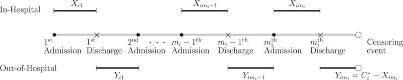
An illustration of a typical alternating recurrent event process.

3. Estimation Methods

3.1. A Brief Review of an Existing Method for Bivariate Non-Recurrent Gap Time Data

We first consider model estimation based on the first bivariate gap time pairs $\left\{\left(X_{i1},Y_{i1},{\mathrm{\Delta }}_{i1}^X,{\mathrm{\Delta }}_{i1}^Y\right);i=1,\dots ,n\right\}$ by adapting the methods for multi-state model developed by Huang [19] to our data structure. For the sake of simplicity, we suppress the order of gap time pairs and use $\left(X_i,Y_i,{\mathrm{\Delta }}_i^X,{\mathrm{\Delta }}_i^Y\right)$ in notation to denote the first pair throughout this section.

Model (1) implies that, given the covariate values A_i and ${\mathbf{A}}_{i\prime }$ for any two subjects i and i′, the two transformed random variables $\log X_i^0-{\mathbf{A}}_i^{\top }{\mathit{\beta }}_1+{\mathbf{A}}_{i\prime }^{\top }{\mathit{\beta }}_1$ and $\log X_{i\prime }^0$ have the same distribution. Define the transformed gap time $X_{ii\prime }^0\left({\mathbf{b}}_1\right)=\text{exp}\left({\mathbf{A}}_{ii\prime }^{\top }{\mathbf{b}}_1\right)X_i^0$, where ${\mathbf{A}}_{ii\prime }={\mathbf{A}}_{i\prime }-{\mathbf{A}}_i$ is the contrast between subjects i and i′ in terms of baseline covariates. It is easy to see that, given A_i and ${\mathbf{A}}_{i\prime }$, $\left\{X_i^0,X_{ii\prime }^0\left({\mathit{\beta }}_1\right)\right\}$ and $\left\{X_{i\prime i}^0\left({\mathit{\beta }}_1\right),X_{i\prime }^0\right\}$ have the same joint distribution when β₁ is the true regression parameter. Let O_L(·,·) be a symmetric, continuous function on {(t, s) : 0 ≤ t ≤ L, 0 ≤ s ≤ L}, where O_L(s, t) is monotonic in t given s and vice versa. By symmetry of O_L, we have

$$\mathrm{E}\left[{\mathbf{A}}_{ii\prime }{O}_L\left\{X_i^0,X_{ii\prime }^0\left({\mathit{\beta }}_1\right)\right\}\right]=0.$$ (3)

Next, we define $Z_i^0=X_i^0+Y_i^0$, the elapse time between the first two consecutive hospital admissions, and the transformed gap time $Z_{ii\prime }^0\left(\mathbf{b}\right)=\exp \left({\mathbf{A}}_{ii\prime }^{\top }{\mathbf{b}}_1\right)X_i^0+\exp \left({\mathbf{A}}_{ii\prime }^{\top }{\mathbf{b}}_2\right)Y_i^0$, where $\mathbf{b}={\left({\mathbf{b}}_1^{\top },{\mathbf{b}}_2^{\top }\right)}^{\top }$. Arguing as before, conditional on A_i and ${\mathbf{A}}_{i\prime }$, $\left\{Z_i^0,Z_{ii\prime }^0\left(\mathit{\beta }\right)\right\}$ and $\left\{Z_{i\prime i}^0\left(\mathit{\beta }\right),Z_{i\prime }^0\right\}$ share the same joint distribution, where $\mathit{\beta }={\left({\mathit{\beta }}_1^{\top },{\mathit{\beta }}_2^{\top }\right)}^{\top }$ are the true regression parameters. Then, it follows that

$$\mathrm{E}\left[{\mathbf{A}}_{ii\prime }{O}_L\left\{Z_i^0,Z_{ii\prime }^0\left(\mathit{\beta }\right)\right\}\right]=0.$$ (4)

In the absence of censoring, estimating equations using observed data can be constructed directly based on (3) and (4). Under right censoring, we define $Z_i=\min \left(Z_i^0,C_i\right)$ the time from the first hospital admission to the next hospital admission or censoring. Analogously, the observed counterparts of $X_{ii\prime }^0$ and $Z_{ii\prime }^0$ are defined as $X_{ii\prime }\left({\mathbf{b}}_1\right)=\exp \left({\mathbf{A}}_{ii\prime }^{\top }{\mathbf{b}}_1\right)X_i$ and $Z_{ii\prime }\left(\mathbf{b}\right)=\exp \left({\mathbf{A}}_{ii\prime }^{\top }{\mathbf{b}}_1\right)X_i+\exp \left({\mathbf{A}}_{ii\prime }^{\top }{\mathbf{b}}_2\right)Y_i$, respectively. Under the independent censoring assumption, we derive

$$\mathrm{E}\left[\frac{{\mathrm{\Delta }}_i^X{O}_L\left\{X_i,X_{ii\prime }\left({\mathit{\beta }}_1\right)\right\}}{G\left(X_i\wedge L\right)}|{\mathbf{A}}_i,{\mathbf{A}}_{i\prime }\right]=\mathrm{E}\left[O_L\left\{X_i^0,X_{ii\prime }^0\left({\mathit{\beta }}_1\right)\right\}|{\mathbf{A}}_i,{\mathbf{A}}_{i\prime }\right],$$

$$\mathrm{E}\left[\frac{{\mathrm{\Delta }}_i^X{O}_L\left\{Z_i,Z_{ii\prime }\left(\mathit{\beta }\right)\right\}}{G\left(Z_i\wedge L\right)}|{\mathbf{A}}_i,{\mathbf{A}}_{i\prime }\right]=\mathrm{E}\left[O_L\left\{Z_i^0,Z_{ii\prime }^0\left(\mathit{\beta }\right)\right\}|{\mathbf{A}}_i,{\mathbf{A}}_{i\prime }\right],$$

by the idea of inverse probability of censoring weights, where a ⋀ b = min(a, b). Following (3) and (4), unconditional on A_i and ${\mathbf{A}}_{i\prime }$, we have

$$\mathrm{E}\left[{\mathbf{A}}_{ii\prime }\frac{{\mathrm{\Delta }}_i^X{O}_L\left\{X_i,X_{ii\prime }\left({\mathit{\beta }}_1\right)\right\}}{G\left(X_i\wedge L\right)}\right]=0,$$ (5)

$$\mathrm{E}\left[{\mathbf{A}}_{ii\prime }\frac{{\mathrm{\Delta }}_i^Y{O}_L\left\{Z_i,Z_{ii\prime }\left(\mathit{\beta }\right)\right\}}{G\left(Z_i\wedge L\right)}\right]=0.$$ (6)

Then, a system of estimating functions can be constructed with the observed bivariate gap times:

$$D_1\left({\mathbf{b}}_1\right)=n^{-2}{\displaystyle \sum _{i=1}^n\left[{\displaystyle \sum _{i\prime =1}^n{\mathbf{A}}_{ii\prime }}\frac{{\mathrm{\Delta }}_i^X{O}_{L_1}\left\{X_i,X_{ii\prime }\left({\mathbf{b}}_1\right)\right\}}{{\widehat{G}}_1\left(X_i\wedge L_1\right)}\right]},$$ (7)

$$D_2\left(\mathbf{b}\right)=n^{-2}{\displaystyle \sum _{i=1}^n\left[{\displaystyle \sum _{i\prime =1}^n{\mathbf{A}}_{ii\prime }}\frac{{\mathrm{\Delta }}_i^Y{O}_{L_2}\left\{Z_i,Z_{ii\prime }\left(\mathbf{b}\right)\right\}}{{\widehat{G}}_2\left(Z_i\wedge L_2\right)}\right]},$$ (8)

where ${\widehat{G}}_1$ and ${\widehat{G}}_2$ are the Kaplan-Meier estimators of the survival function G(·) based on the data $\left\{\left(X_i,1-{\mathrm{\Delta }}_i^X\right),i=1,\dots ,n\right\}$ and $\left\{\left(Z_i,1-{\mathrm{\Delta }}_i^Y\right),i=1,\dots ,n\right\}$, respectively. As pointed out in [19], ${\widehat{G}}_2$ can be used in (7) in place of ${\widehat{G}}_1$, but this often leads to a greater variance of D₁(b₁). The limits L₁ < τ_C and L₂ < τ_C are imposed to address the problem of $X_i^0$ and $Z_i^0$ having maximum support greater than τ_C. One can inductively solve the estimating equations D₁(b₁) = 0 and D₂ (b) = 0 to obtain the estimates for β₁ and β₂. Conventional methods for survival analysis under the AFT model (see [22], and reference therein) are not directly applicable to the estimation of Model (2). In our setting, the break period $Y_i^0$ is subject to induced dependent censoring because it is censored by max $\left(C_i-X_i^0,0\right)$, which is informative due to the correlation between $X_i^0$ and $Y_i^0$. By considering the elapse time between consecutive admissions $Z_i^0$ and the sum of transformed care and break periods $Z_{ii\prime }^0$ instead of the break period $Y_i^0$ solely, we circumvent the induced dependent censoring issue.

3.2. The Proposed Estimation Method

We now extend the method in Section 3.1 to deal with alternating recurrent gap time data. As pointed out in [2], the m_i th pair of gap times tends to be longer than the uncensored pairs of gap times due to bias induced by intercept sampling (also see [20], p.65 for the example of textile fiber sampling). As a result, naively including all observed data in the estimation procedure usually leads to inconsistent estimation. In this section we extend the method for multi-state models proposed by Huang [19], which was reviewed in Section 3.1, to the setting of alternating recurrent events.

Define $m_i^{\ast }=\max \left(m_i-1,1\right)$. Thus for patients with no completely observed bivariate gap time pairs, $m_i^{\ast }=1$; for patients with at least one completely observed gap time pair, $m_i^{\ast }$ is the number of complete pairs. Let the elapse time between two consecutive hospital admissions be denoted as $Z_{ij}^0=X_{ij}^0+Y_{ij}^0$ and its observed counterparts as $Z_{ij}=X_{ij}+Y_{ij}$, for j = 1,…, $m_i^{\ast }$. The observed transformed times are defined as

$$X_{ii\prime j}\left({\mathbf{b}}_1\right)=\exp \left({\mathbf{A}}_{ii\prime }^{\top }{\mathbf{b}}_1\right)X_{ij},$$

$$Z_{ii\prime j}\left(\mathbf{b}\right)=\exp \left({\mathbf{A}}_{ii\prime }^{\top }{\mathbf{b}}_1\right)X_{ij}+\exp \left({\mathbf{A}}_{ii\prime }^{\top }{\mathbf{b}}_2\right)Y_{ij},j=1,\dots ,m_i^{\ast }.$$

Under our model assumption, conditioning on m_i, γ_i, and A_i, the observed bivariate pairs, $\left(X_{i1},Y_{i1}\right),\dots ,\left(X_{i{m}_i^{\ast }},Y_{i{m}_{{ }_i}^{\ast }}\right)$ are i.i.d. when m_i ≥ 2. Thus, replacing $\left\{X_i,X_{ii\prime }\left({\mathit{\beta }}_1\right),Z_i,Z_{ii\prime }\left(\mathit{\beta }\right)\right\}$ with $\left\{X_{ij},X_{ii\prime j}\left({\mathit{\beta }}_1\right),Z_{ij},Z_{ii\prime j}\left(\mathit{\beta }\right)\right\}$ for any $j=1,\dots ,m_i^{\ast }$ in (5) and (6) should give unbiased estimating equations. We propose to apply the idea of weighted risk-set method [11] to assign a weight $1/m_i^{\ast }$ to each pair of bivariate gap times and sum over $j=1,\dots ,m_i^{\ast }$ to construct more efficient estimating functions. Specifically, arguing as in [11], we can prove that the weighted averages of $O_{L_1}\left(·,·\right)$ and $O_{L_2}\left(·,·\right)$ over the conditional i.i.d. bivariate pairs have the same expectations as their counterparts for the first bivariate gap time pair only data:

$$\mathrm{E}\left(\frac{1}{m_i^{\ast }}{\displaystyle \sum _{j=1}^{m_i^{\ast }}\mathrm{E}}\left[\frac{{\mathrm{\Delta }}_{ij}^X{O}_L\left\{X_{ij},X_{ii\prime j}\left({\mathit{\beta }}_1\right)\right\}}{G\left(X_{ij}\wedge L\right)}|m_i^{\ast },{\mathit{\gamma }}_i,{\mathbf{A}}_i,{\mathbf{A}}_{i\prime }\right]|{\mathbf{A}}_i,{\mathbf{A}}_{i\prime }\right)=\mathrm{E}\left[\frac{{\mathrm{\Delta }}_{i1}^X{O}_L\left\{X_{i1,}{X}_{ii\prime 1}\left({\mathit{\beta }}_1\right)\right\}}{G\left(X_{i1}\wedge L\right)}|{\mathbf{A}}_i,{\mathbf{A}}_{i\prime }\right],$$

$$\mathrm{E}\left(\frac{1}{m_i^{\ast }}{\displaystyle \sum _{j=1}^{m_i^{\ast }}\mathrm{E}}\left[\frac{{\mathrm{\Delta }}_{ij}^Y{O}_L\left\{Z_{ij},Z_{ii\prime j}\left(\mathit{\beta }\right)\right\}}{G\left(Z_{ij}\wedge L\right)}|m_i^{\ast },{\mathit{\gamma }}_i,{\mathbf{A}}_i,{\mathbf{A}}_{i\prime }\right]|{\mathbf{A}}_i,{\mathbf{A}}_{i\prime }\right)=\mathrm{E}\left[\frac{{\mathrm{\Delta }}_{i1}^Y{O}_L\left\{Z_{i1,}{Z}_{ii\prime 1}\left(\mathit{\beta }\right)\right\}}{G\left(Z_{i1}\wedge L\right)}|{\mathbf{A}}_i,{\mathbf{A}}_{i\prime }\right].$$

It follows directly that

$$\mathrm{E}\left[{\mathbf{A}}_{ii\prime }\frac{1}{m_i^{\ast }}{\displaystyle \sum _{j=1}^{m_i^{\ast }}\frac{{\mathrm{\Delta }}_{ij}^X{O}_L\left\{X_{ij},X_{ii\prime j}\left({\mathit{\beta }}_1\right)\right\}}{G\left(X_{ij}\wedge L\right)}}\right]=0,$$ (9)

$$\mathrm{E}\left[{\mathbf{A}}_{ii\prime }\frac{1}{m_i^{\ast }}{\displaystyle \sum _{j=1}^{m_i^{\ast }}\frac{{\mathrm{\Delta }}_{ij}^Y{O}_L\left\{Z_{ij},Z_{ii\prime j}\left(\mathit{\beta }\right)\right\}}{G\left(Z_{ij}\wedge L\right)}}\right]=0.$$ (10)

By using data only up to the $m_i^{\ast }$ th pair in the above formulation for subjects who have at least one completely observed gap time pair, we exclude the potentially longer gap time pairs and avoid intercept sampling bias. Hence, $X_{i{m}_i}$, either censored or uncensored, and $Y_{i{m}_i}$, which is always censored, are not used for such subjects in (9) and (10). For subjects who have no completely observed gap time pairs, we only use their data for constructing consistent estimators for G(·) if the first gap time is censored (i.e., ${\mathrm{\Delta }}_{i1}^X=0$), otherwise (i.e., ${\mathrm{\Delta }}_{i1}^X=1$) the data of such subjects are used in both the estimation of G(·) and the numerator in the expectation in (9). Therefore, we can construct a system of estimating functions as follows:

$$D_1^{\ast }\left({\mathbf{b}}_1\right)=n^{-2}{\displaystyle \sum _{i=1}^n\left[{\displaystyle \sum _{i\prime =1}^n{\mathbf{A}}_{ii\prime }}\frac{1}{m_i^{\ast }}{\displaystyle \sum _{j=1}^{m_i^{\ast }}\frac{{\mathrm{\Delta }}_{ij}^X{O}_{L_1}\left\{X_{ij},X_{ii\prime j}\left({\mathbf{b}}_1\right)\right\}}{{\widehat{G}}_1\left(X_{ij}\wedge L_1\right)}}\right]},$$ (11)

$$D_2^{\ast }\left(\mathbf{b}\right)=n^{-2}{\displaystyle \sum _{i=1}^n\left[{\displaystyle \sum _{i\prime =1}^n{\mathbf{A}}_{ii\prime }}\frac{1}{m_i^{\ast }}{\displaystyle \sum _{j=1}^{m_i^{\ast }}\frac{{\mathrm{\Delta }}_{ij}^Y{O}_{L_2}\left\{Z_{ij},Z_{ii\prime j}\left(\mathbf{b}\right)\right\}}{{\widehat{G}}_2\left(Z_{ij}\wedge L_2\right)}}\right]},$$ (12)

where ${\widehat{G}}_1$ and ${\widehat{G}}_2$ are Kaplan-Meier estimators based on the first pair of bivariate gap times (censored or uncensored) as in (7) and (8). The proposed estimators ${\widehat{\mathit{\beta }}}_1$ and ${\widehat{\mathit{\beta }}}_2$ can be obtained by inductively solving $D_1^{\ast }\left({\mathbf{b}}_1\right)=0$ and $D_2^{\ast }\{{\left({\widehat{\mathit{\beta }}}_1^{\top }{\mathbf{b}}_2^{\top }\right)}^{\top }\}=0$. Following [19], we choose O_L (t, s) = log [min{max(t, s), L}] − log(L) to yield monotonic estimating functions which guarantee a unique solution. Further discussions on the selection of O_L can be found in [19]. Compared with the method for bivariate non-recurrent gap time data reviewed in Section 3.1, the proposed estimation method is expected to be more efficient because the information beyond the second hospital admission time of each patient is utilized.

3.3. Asymptotic Properties

In this section, we establish the consistency and the asymptotic normality of the proposed estimator $\widehat{\mathit{\beta }}={\left({\widehat{\mathit{\beta }}}_1^{\top },{\widehat{\mathit{\beta }}}_2^{\top }\right)}^{\top }$. Following Huang [19], we begin by rewriting the estimating functions (7) and (8) as

$$D_1\left({\mathbf{b}}_1\right)={\displaystyle {\int }_{t,s,{\mathbf{a}}_1,{\mathbf{a}}_2}\left({\mathbf{a}}_2-{\mathbf{a}}_1\right)}\frac{O_{L_1}\left(t,s\right)}{{\widehat{G}}_1\left(t\wedge L_1\right)}{\widehat{F}}_1\left(\mathrm{d}t,\mathrm{d}s,\mathrm{d}{\mathbf{a}}_1;{\mathbf{a}}_2,{\mathbf{b}}_1\right)\widehat{H}\left(\mathrm{d}{\mathbf{a}}_2\right),$$ (13)

$$D_2\left(\mathbf{b}\right)={\displaystyle {\int }_{t,s,{\mathbf{a}}_1,{\mathbf{a}}_2}\left({\mathbf{a}}_2-{\mathbf{a}}_1\right)}\frac{O_{L_2}\left(t,s\right)}{{\widehat{G}}_2\left(t\wedge L_2\right)}{\widehat{F}}_2\left(\mathrm{d}t,\mathrm{d}s,\mathrm{d}{\mathbf{a}}_1;{\mathbf{a}}_2,\mathbf{b}\right)\widehat{H}\left(\mathrm{d}{\mathbf{a}}_2\right),$$ (14)

where ${\widehat{F}}_1$, ${\widehat{F}}_2$, and $\widehat{H}$ are the empirical estimators of

$$F_1\left(t,s,{\mathbf{a}}_1;{\mathbf{a}}_2,{\mathbf{b}}_1\right)=\mathrm{Pr}\left[X_{i1}\le t,\exp \left\{{\left({\mathbf{a}}_2-{\mathbf{A}}_i\right)}^{\top }{\mathbf{b}}_1\right\}{X}_{i1}\le s,{\mathbf{A}}_i\le {\mathbf{a}}_1,{\mathrm{\Delta }}_{i1}^X=1\right],$$

$$F_2\left(t,s,{\mathbf{a}}_1;{\mathbf{a}}_2,\mathbf{b}\right)=\mathrm{Pr}\left[Z_{i1}\le t,\exp \left\{{\left({\mathbf{a}}_2-{\mathbf{A}}_i\right)}^{\top }{\mathbf{b}}_1\right\}{X}_{i1}+\exp \left\{{\left({\mathbf{a}}_2-{\mathbf{A}}_i\right)}^{\top }{\mathbf{b}}_2\right\}{Y}_{i1}\le s,{\mathbf{A}}_i\le {\mathbf{a}}_1,{\mathrm{\Delta }}_{i2}^X=1\right],$$

and H(a₂) = Pr(A_i ≤ a₂), respectively. Note that Pr(A_i ≤ a) = Pr(A_i1 ≤ a₁,…,A_ip ≤ a_p), where A_i = (A_i1,…, A_ip)^⊤ and a = (a₁,…, a_p)^⊤. Huang showed that D₁ and D₂ are continuous and compactly differentiable functionals through the properties of the components, ${\widehat{G}}_1$, ${\widehat{G}}_2$, ${\widehat{F}}_1$, ${\widehat{F}}_2$, and $\widehat{H}$. Based on the re-expression in (13) and (14), both $D_1^{\top }\left({\mathbf{b}}_1\right)\left({\mathbf{b}}_1-{\mathit{\beta }}_1\right)$ and $D_2^{\top }\left(\mathbf{b}\right)\left({\mathbf{b}}_2-{\mathit{\beta }}_2\right)$ converge almost surely and uniformly in b₁ and in b to

$$\mathrm{E}\left[{\mathbf{A}}_{ii\prime }^{\top }\left({\mathbf{b}}_1-{\mathit{\beta }}_1\right)O_{L_1}\left\{X_{i1}^0,X_{ii\prime 1}^0\left({\mathbf{b}}_1\right)\right\}\right]\text{and}$$ (15)

$$\mathrm{E}\left[{\mathbf{A}}_{ii\prime }^{\top }\left({\mathbf{b}}_2-{\mathit{\beta }}_2\right)O_{L_2}\left\{Z_{i1}^0,Z_{ii\prime 1}^0\left(\mathbf{b}\right)\right\}\right],$$ (16)

respectively. It can be shown that the estimating functions $D_1^{\ast }$ and $D_2^{\ast }$ in (11) and (12) converge uniformly to the same limit as D₁ and D₂, respectively. Thus, it follows that $D_1^{\ast }{ }^{\top }\left({\mathbf{b}}_1\right)\left({\mathbf{b}}_1-{\mathit{\beta }}_1\right)$ and $D_2^{\ast }{ }^{\top }\left(\mathbf{b}\right)\left({\mathbf{b}}_2-{\mathit{\beta }}_2\right)$ also converge almost surely to (15) and (16). Since (15) equals 0 when b₁= β₁, ${\widehat{\mathit{\beta }}}_1$ is consistent for β₁. Given the consistency of ${\widehat{\mathit{\beta }}}_1$, the consistency of ${\widehat{\mathit{\beta }}}_2$ follows from the fact that (16) equals 0 when b₂ = β₂.

To prove the asymptotic normality of $\widehat{\mathit{\beta }}$, it suffices to establish the asymptotic normality and linearity of $D^{\ast }\left(\mathit{\beta }\right)={\left\{D_1^{\ast }{ }^{\top }\left({\mathit{\beta }}_1\right),D_2^{\ast }{ }^{\top }\left(\mathit{\beta }\right)\right\}}^{\top }$. Huang [19] showed that n^1/2 D(β) is asymptotically normal with mean zero and variance Ω using the compact differentiability of (13) and (14), where $D\left(\mathit{\beta }\right)={\left\{D_1^{\top }\left({\mathit{\beta }}_1\right),D_2^{\top }\left(\mathit{\beta }\right)\right\}}^{\top }$. For the variance, we define

$${\xi }_{i1}\left({\mathit{\beta }}_1\right)=n^{-3/2}{\displaystyle \sum _{i\prime =1}^n{\mathbf{A}}_{ii\prime }}\left[\frac{{\mathrm{\Delta }}_{i1}^X{O}_{L_1}\left\{X_{i1},X_{ii\prime 1}\left({\mathit{\beta }}_1\right)\right\}}{{\widehat{G}}_1\left(X_{i1}\wedge L_1\right)}-\frac{{\mathrm{\Delta }}_{i\prime 1}^X{O}_{L_1}\left\{X_{i\prime 1},X_{i\prime i1}\left({\mathit{\beta }}_1\right)\right\}}{{\widehat{G}}_1\left(X_{i\prime 1}\wedge L_1\right)}\right]+n^{-3/2}{\displaystyle {\int }_0^{L_1}\frac{U_1\left(t,{\mathit{\beta }}_1\right){\widehat{G}}_1\left(t-\right)}{R_1\left(t\right){\widehat{G}}_1\left(t\right)}}\mathrm{d}{\widehat{M}}_{i1}\left(t\right),$$

$$\begin{gathered} {\xi }_{i2}\left(\mathit{\beta }\right)=n^{-3/2}{\displaystyle \sum _{i\prime =1}^n{\mathbf{A}}_{ii\prime }}\left[\frac{{\mathrm{\Delta }}_{i1}^Y{O}_{L_2}\left\{Z_{i1},Z_{ii\prime 1}\left(\mathit{\beta }\right)\right\}}{{\widehat{G}}_2\left(Z_{i1}\wedge L_2\right)}-\frac{{\mathrm{\Delta }}_{i\prime 1}^Y{O}_{L_2}\left\{Z_{i\prime 1},Z_{i\prime i1}\left(\mathit{\beta }\right)\right\}}{{\widehat{G}}_2\left(Z_{i\prime 1}\wedge L_2\right)}\right] \\ +n^{-3/2}{\displaystyle {\int }_0^{L_2}\frac{U_2\left(t,\mathit{\beta }\right){\widehat{G}}_2\left(t-\right)}{R_2\left(t\right){\widehat{G}}_2\left(t\right)}}\mathrm{d}{\widehat{M}}_{i2}\left(t\right), \end{gathered}$$

in which

$$U_1\left(t,{\mathit{\beta }}_1\right)={\displaystyle \sum _{i=1}^n{\displaystyle \sum _{i\prime =1}^n{\mathbf{A}}_{ii\prime }}}\left[\frac{{\mathrm{\Delta }}_{i1}^X{O}_{L_1}\left\{X_{i1},X_{ii\prime 1}\left({\mathit{\beta }}_1\right)\right\}}{{\widehat{G}}_1\left(X_{i1}\wedge L_1\right)}I\left(X_{i1}>t\right)\right],$$

$$U_2\left(t,\mathit{\beta }\right)={\displaystyle \sum _{i=1}^n{\displaystyle \sum _{i\prime =1}^n{\mathbf{A}}_{ii\prime }}}\left[\frac{{\mathrm{\Delta }}_{i1}^X{O}_{L_2}\left\{Z_{i1},Z_{ii\prime 1}\left(\mathit{\beta }\right)\right\}}{{\widehat{G}}_2\left(Z_{i1}\wedge L_2\right)}I\left(Z_{i1}>t\right)\right],$$

$R_1\left(t\right)={\displaystyle {\sum }_{i=1}^{n}I\left(X_{i1}\ge t\right)}$, $R_2\left(t\right)={\displaystyle {\sum }_{i=1}^{n}I\left(Z_{i1}\ge t\right)}$, ${\widehat{M}}_{i1}\left(t\right)=I\left(X_{i1}\le t,{\mathrm{\Delta }}_{i1}^X=0\right)-{\displaystyle {\int }_0^{t}I}\left(X_{i1}\ge s\right)\mathrm{d}{\widehat{\mathrm{\Lambda }}}_1\left(s\right)$, ${\widehat{M}}_{i2}\left(t\right)=I\left(Z_{i1}\le t,{\mathrm{\Delta }}_{i1}^Y=0\right)-{\displaystyle {\int }_0^{t}I}\left(Z_{i1}\ge s\right)\mathrm{d}{\widehat{\mathrm{\Lambda }}}_2\left(s\right)$, and ${\widehat{\mathrm{\Lambda }}}_1$ and ${\widehat{\mathrm{\Lambda }}}_2$ are the Nelson–Aalen estimator corresponding to ${\widehat{G}}_1$ and ${\widehat{G}}_2$, respectively. The variance Ω is the limit of ${{\displaystyle {\sum }_{i=1}^n\left\{{\xi }_{i1}^{\top }\left({\mathit{\beta }}_1\right),{\xi }_{i2}^{\top }\left(\mathit{\beta }\right)\right\}}}^{\top }\left\{{\xi }_{i1}^{\top }\left({\mathit{\beta }}_1\right),{\xi }_{i2}^{\top }\left(\mathit{\beta }\right)\right\}$. Now, we show the asymptotic normality of D*(β) following the approach in [19]. We note that $D_1^{\ast }$ and $D_2^{\ast }$ are continuous and compactly differentiable. By applying the functional delta method and the influence function approach, n^1/2 D*(β) converges weakly to a normal distribution with mean zero and variance Ω*. Define

$${\xi }_{i1}^{\ast }\left({\mathit{\beta }}_1\right)=n^{-3/2}{\displaystyle \sum _{i\prime =1}^n{\mathbf{A}}_{ii\prime }}\left[\frac{1}{m_i^{\ast }}{\displaystyle \sum _{j=1}^{m_i^{\ast }}\frac{{\mathrm{\Delta }}_{ij}^X{O}_{L_1}\left\{X_{ij},X_{ii\prime j}\left({\mathit{\beta }}_1\right)\right\}}{{\widehat{G}}_1\left(X_{ij}\wedge L_1\right)}}-\frac{1}{m_{i\prime }^{\ast }}{\displaystyle \sum _{l=1}^{m_{i\prime }^{\ast }}\frac{{\mathrm{\Delta }}_{i\prime l}^X{O}_{L_1}\left\{X_{i\prime l},X_{i\prime il}\left({\mathit{\beta }}_1\right)\right\}}{{\widehat{G}}_1\left(X_{i\prime l}\wedge L_1\right)}}\right]+n^{-3/2}{\displaystyle {\int }_0^{L_1}\frac{U_1^{\ast }\left(t,{\mathit{\beta }}_1\right){\widehat{G}}_1\left(t-\right)}{R_1^{\ast }\left(t\right){\widehat{G}}_1\left(t\right)}}\mathrm{d}{\widehat{M}}_{i1}^{\ast }\left(t\right),$$

$${\xi }_{i2}^{\ast }\left(\mathit{\beta }\right)=n^{-3/2}{\displaystyle \sum _{i\prime =1}^n{\mathbf{A}}_{ii\prime }}\left[\frac{1}{m_i^{\ast }}{\displaystyle \sum _{j=1}^{m_i^{\ast }}\frac{{\mathrm{\Delta }}_{ij}^X{O}_{L_2}\left\{Z_{ij},Z_{ii\prime j}\left(\mathit{\beta }\right)\right\}}{{\widehat{G}}_2\left(Z_{ij}\wedge L_2\right)}}-\frac{1}{m_{i\prime }^{\ast }}{\displaystyle \sum _{l=1}^{m_{i\prime }^{\ast }}\frac{{\mathrm{\Delta }}_{i\prime l}^X{O}_{L_2}\left\{Z_{i\prime l},Z_{i\prime il}\left(\mathit{\beta }\right)\right\}}{{\widehat{G}}_2\left(Z_{i\prime l}\wedge L_2\right)}}\right]+n^{-3/2}{\displaystyle {\int }_0^{L_2}\frac{U_2^{\ast }\left(t,\mathit{\beta }\right){\widehat{G}}_2\left(t-\right)}{R_2^{\ast }\left(t\right){\widehat{G}}_2\left(t\right)}}\mathrm{d}{\widehat{M}}_{i2}^{\ast }\left(t\right),$$

in which,

$$U_1^{\ast }\left(t,{\beta }_1\right)={\displaystyle \sum _{i=1}^n{\displaystyle \sum _{i\prime =1}^n{\mathbf{A}}_{ii\prime }}}\left[\frac{1}{m_i^{\ast }}{\displaystyle \sum _{j=1}^{m_i^{\ast }}\frac{{\mathrm{\Delta }}_{ij}^X{O}_{L_1}\left\{X_{ij},X_{ii\prime j}\left({\mathit{\beta }}_1\right)\right\}}{{\widehat{G}}_1\left(X_{ij}\wedge L_1\right)}I\left(X_{ij}>t\right)}\right],$$

$$U_2^{\ast }\left(t,\beta \right)={\displaystyle \sum _{i=1}^n{\displaystyle \sum _{i\prime =1}^n{\mathbf{A}}_{ii\prime }}}\left[\frac{1}{m_i^{\ast }}{\displaystyle \sum _{j=1}^{m_i^{\ast }}\frac{{\mathrm{\Delta }}_{ij}^Y{O}_{L_2}\left\{Z_{ij},Z_{ii\prime j}\left(\mathit{\beta }\right)\right\}}{{\widehat{G}}_2\left(Z_{ij}\wedge L_2\right)}I\left(Z_{ij}>t\right)}\right],$$

$R_1^{\ast }\left(t\right)={\displaystyle {\sum }_{i=1}^n{\displaystyle {\sum }_{j=1}^{m_i^{\ast }}I\left(X_{ij}\ge t\right)}}/m_i^{\ast }$, $R_2^{\ast }\left(t\right)={\displaystyle {\sum }_{i=1}^n{\displaystyle {\sum }_{j=1}^{m_i^{\ast }}I\left(Z_{ij}\ge t\right)}}/m_i^{\ast }$, ${\widehat{M}}_{i1}^{\ast }\left(t\right)={\displaystyle {\sum }_{j=1}^{m_i^{\ast }}I\left(X_{ij}\le t,{\mathrm{\Delta }}_{ij}^X=0\right)/m_i^{\ast }-{\displaystyle {\int }_0^t{\displaystyle {\sum }_{j=1}^{m_i^{\ast }}I\left(X_{ij}\ge s\right)/m_i^{\ast }}\mathrm{d}{\widehat{\mathrm{\Lambda }}}_1\left(s\right)}}$, and ${\widehat{M}}_{i2}^{\ast }\left(t\right)={\displaystyle {\sum }_{j=1}^{m_i^{\ast }}I\left(Z_{ij}\le t,{\mathrm{\Delta }}_{ij}^Y=0\right)}/m_i^{\ast }-{\displaystyle {\int }_0^t{\displaystyle {\sum }_{j=1}^{m_i^{\ast }}I\left(Z_{ij}\ge s\right)/m_i^{\ast }\mathrm{d}{\widehat{\mathrm{\Lambda }}}_2}\left(s\right)}$. By exchangeability, the weighted average ${\xi }_{ik}^{\ast }$, $U_k^{\ast }$, $R_k^{\ast }$, and $M_{ik}^{\ast }$ converge uniformly to the same limit as their counterparts, ξ_ik, U_k, R_k, and M_ik, for k = 1,2. Thus, the variance Ω* can be estimated by ${\widehat{\mathrm{\Omega }}}^{\ast }={{\displaystyle {\sum }_{i=1}^n\left\{{\xi }_{i1}^{\ast \top }\left({\widehat{\mathit{\beta }}}_1\right),{\xi }_{i2}^{\ast \top }\left(\widehat{\mathit{\beta }}\right)\right\}}}^{\top }\left\{{\xi }_{i1}^{\ast \top }\left({\widehat{\mathit{\beta }}}_1\right),{\xi }_{i2}^{\ast \top }\left(\widehat{\mathit{\beta }}\right)\right\}$. By the Glivenko-Cantelli theorem in [23], ${{\displaystyle {\sum }_{i=1}^n\left\{{\xi }_{i1}^{\ast \top }\left({\mathbf{b}}_1\right),{\xi }_{i2}^{\ast \top }\left(\mathbf{b}\right)\right\}}}^{\top }\left\{{\xi }_{i1}^{\ast \top }\left({\mathbf{b}}_1\right),{\xi }_{i2}^{\ast \top }\left(\mathbf{b}\right)\right\}$ converges uniformly and almost surely in b to a limiting function continuous at b = β. Hence, the variance estimate ${\widehat{\mathrm{\Omega }}}^{\ast }$ is consistent for Ω* given the consistency of $\widehat{\mathit{\beta }}$.

The estimating functions (11) and (12) can be rewritten as ${\overline{D}}_1^{\ast }\left({\mathbf{b}}_1\right)$ and ${\overline{D}}_2^{\ast }\left(\mathbf{b}\right)$ by replacing ${\widehat{F}}_1$ and ${\widehat{F}}_2$ in (13) and (14) with their weighted counterparts

$$\frac{1}{n}{\displaystyle \sum _{i=1}^n\frac{1}{m_i^{\ast }}}{\displaystyle \sum _{j=1}^{m_i^{\ast }}I\left[X_{ij}\le t,\exp \left\{{\left({\mathbf{a}}_2-\mathbf{A}\right)}^{\top }{\mathbf{b}}_1\right\}{X}_{ij}\le s,\mathbf{A}\le {\mathbf{a}}_1,{\mathrm{\Delta }}_{ij}^X=1\right]}\text{and}\frac{1}{n}{\displaystyle \sum _{i=1}^n\frac{1}{m_i^{\ast }}}{\displaystyle \sum _{j=1}^{m_i^{\ast }}I}\left[Z_{ij}\le t,\exp \left\{{\left({\mathbf{a}}_2-\mathbf{A}\right)}^{\top }{\mathbf{b}}_1\right\}{X}_{ij}+\exp \left\{{\left({\mathbf{a}}_2-\mathbf{A}\right)}^{\top }{\mathbf{b}}_2\right\}{Y}_{ij}\le s,\mathbf{A}\le {\mathbf{a}}_1,{\mathrm{\Delta }}_{ij}^Y=1\right],$$

respectively. We note that ${\overline{D}}^{\ast }\left(\mathbf{b}\right)={\left\{{\overline{D}}_1^{\ast }{ }^{\top }\left({\mathbf{b}}_1\right),{\overline{D}}_2^{\ast }{ }^{\top }\left(\mathbf{b}\right)\right\}}^{\top }$ is not everywhere differentiable. Thus, the first-order Taylor expansion cannot be directly used. Instead, we use the generalized law of mean, proposed in [24], to accommodate the nondifferentiable functions. By applying the generalized law of mean, we have

$$D^{\ast }\left(\mathbf{b}\right)={\overline{D}}^{\ast }\left(\mathbf{b}\right)+o_p\left(\Vert \mathbf{b}-\mathit{\beta }\Vert +n^{-1/2}\right)=D^{\ast }\left(\mathit{\beta }\right)+{\displaystyle {\sum }_{\mathit{\beta }}\left(\mathbf{b}-\mathit{\beta }\right)}+o_p\left(\Vert \mathbf{b}-\mathit{\beta }\Vert +n^{-1/2}\right)$$

for b converging to β, where Σ_β is the limit of the left and right partial derivative of ${\overline{D}}^{\ast }\left(\mathit{\beta }\right)$. It follows that D*(b) is asymptotically linear at b = β.

The asymptotic normality of $\widehat{\mathit{\beta }}$ naturally follows from the asymptotic normality and linearity of D* (β). Thus, $n^{1/2}\left(\widehat{\mathit{\beta }}-\mathit{\beta }\right)$ converges weakly to a normal distribution with mean zero and variance consistently estimated by ${\widehat{\sum }}_{\widehat{\mathit{\beta }}}^{-1}{\widehat{\mathrm{\Omega }}}^{\ast }{\left({\widehat{\sum }}_{\widehat{\mathit{\beta }}}^{-1}\right)}^{\top }$ where ${\widehat{\sum }}_{\widehat{\mathit{\beta }}}$ is the derivative matrix of ${\overline{D}}^{\ast }\left(\mathbf{b}\right)$ evaluated at $\mathbf{b}=\widehat{\mathit{\beta }}$.

4. Simulation Studies

We conducted a series of simulation studies to assess the performance of the proposed method. For each setting, we simulated 1000 datasets with sample sizes of n = 150 and 300 from the assumed models (1) and (2). Two covariates A = (A₁, A₂)^⊤ are generated from a Bernoulli distribution with probability 0.5 and a uniform distribution (0, 1), respectively. We set the true regression parameters as β₁ = (0.5, 0.5)^⊤ and β₂ = (0, −0.5)^⊤ to account for the distinct covariate effects on the two alternating states. We consider two scenarios where (1) the subject-specific latent vector (γ_i1, γ_i2) follows a bivariate normal distribution with varying levels of correlation; and (2) the latent variables γ_i1 and γ_i2 are from different distributions. The error terms ε_ij1 and ε_ij2 are simulated from independent normal distributions with mean zero and variance 0.1. Since the recurrent event process is subject to right censoring, we generate the censoring time C_i from a uniform distribution that yields 15% or 30% of subjects to have their first bivariate gap time pairs censored on average. Under each setting, we evaluate the performance of the proposed method relative to the rank-based method by Chang [6] (referred to as Chang’s method). For the latter method, we present the perturbation-based variance estimates adopted in the original paper [6]. For both methods, we present the mean of the point estimates (Mean), the empirical standard deviation of the point estimates (SD), the empirical average of the standard error estimates (SE), and the coverage probability based on the 95% confidence intervals (CP).

Simulation Scenario 1

In the first scenario, we generate the subject-specific latent vector (γ_i1, γ_i2) from a bivariate normal distribution with unit mean vector and variance-covariance matrix $\left(\begin{array}{cc}0.5& 0.5\rho \\ 0.5\rho & 0.5\end{array}\right)$ We consider ρ =1,0.5, and 0. When ρ = 1, the two latent variables γ_i1 = γ_i2; when ρ = 0, γ_i1 and γ_i2 are independent. The simulation results are summarized in the upper panels of Tables 1 and 2 for sample sizes of n = 150 and 300, respectively. The proposed estimator provides virtually unbiased point estimates, and the SE’s are close to the SD’s across all settings. The CP’s are reasonably close to the nominal level. We observe that the SD’s and SE’s increase as the censoring rate increases from 15% to 30% because fewer bivariate gap time pairs are observed. We note that the level of association between alternating gap times has little impact on the point estimation or the variance estimation. As expected, the variance decreases with the sample size.

Table 1.

Summary statistics for the simulation study with n = 150.

			Proposed method		Chang’s method
			β1	β2	β1	β2
			A1, A2	A1, A2	A1, A2	A1, A2
ρ	cr	True	0.5, 0.5	0.0, −0.5	0.5, 0.5	0.0, −0.5
Scenario 1
			$\overline{m}=6.36$
1	15%	Mean	0.495, 0.494	−0.031, −0.508	0.486, 0.521	−0.004, −0.408
		SD	0.138, 0.262	0.223, 0.367	0.141, 0.226	0.152, 0.217
		SE	0.140, 0.245	0.219, 0.363	0.144, 0.282	0.170, 0.263
		CP	0.952, 0.930	0.927, 0.924	0.954, 0.985	0.956, 0.961
			$\overline{m}=3.31$
	30%	Mean	0.501, 0.490	−0.026, −0.505	0.487, 0.518	−0.014, −0.404
		SD	0.154, 0.271	0.246, 0.403	0.138, 0.235	0.177, 0.227
		SE	0.150, 0.263	0.243, 0.405	0.155, 0.304	0.207, 0.279
		CP	0.942, 0.934	0.918, 0.915	0.949, 0.973	0.967, 0.958
			$\overline{m}=5.76$
0.5	15%	Mean	0.500, 0.501	−0.004, −0.494	0.489, 0.511	−0.003, −0.414
		SD	0.139, 0.253	0.204, 0.368	0.141, 0.230	0.160, 0.210
		SE	0.140, 0.245	0.208, 0.352	0.140, 0.274	0.176, 0.251
		CP	0.958, 0.940	0.934, 0.925	0.947, 0.959	0.966, 0.952
			$\overline{m}=3.05$
	30%	Mean	0.499, 0.504	−0.016, −0.511	0.487, 0.514	−0.006, −0.404
		SD	0.148, 0.265	0.237, 0.395	0.139, 0.244	0.181, 0.236
		SE	0.150, 0.263	0.235, 0.393	0.149, 0.295	0.215, 0.273
		CP	0.941, 0.949	0.929, 0.927	0.957, 0.960	0.981, 0.941
			$\overline{m}=5.28$
0	15%	Mean	0.498, 0.501	−0.010, −0.490	0.487, 0.464	0.017, −0.416
		SD	0.145, 0.255	0.204, 0.369	0.133, 0.243	0.154, 0.221
		SE	0.140, 0.245	0.208, 0.352	0.140, 0.265	0.179, 0.254
		CP	0.938, 0.945	0.943, 0.928	0.955, 0.950	0.975, 0.945
			$\overline{m}=2.81$
	30%	Mean	0.501, 0.493	−0.013, −0.509	0.477, 0.479	0.002, −0.398
		SD	0.149, 0.274	0.227, 0.405	0.144, 0.268	0.177, 0.254
		SE	0.149, 0.262	0.232, 0.392	0.151, 0.288	0.205, 0.278
		CP	0.961, 0.937	0.942, 0.914	0.961, 0.955	0.966, 0.930
Scenario 2
			$\overline{m}=5.32$
–	15%	Mean	0.500, 0.497	0.000, −0.506	0.498, 0.491	0.015, −0.417
		SD	0.139, 0.249	0.237, 0.404	0.131, 0.259	0.182, 0.252
		SE	0.140, 0.245	0.233, 0.393	0.139, 0.261	0.208, 0.270
		CP	0.954, 0.943	0.930, 0.911	0.959, 0.934	0.964, 0.942
			$\overline{m}=2.90$
	30%	Mean	0.505, 0.495	−0.010, −0.513	0.480, 0.490	0.000, −0.412
		SD	0.149, 0.271	0.250, 0.437	0.140, 0.249	0.195, 0.248
		SE	0.149, 0.261	0.252, 0.424	0.153, 0.280	0.222, 0.282
		CP	0.947, 0.933	0.920, 0.912	0.961, 0.958	0.955, 0.935

True, true coefficients; Mean, empirical average of point estimates; SD, empirical standard deviation of point estimates; SE, empirical average of standard error estimates; CP, coverage probability based on the 95% confidence interval; $\overline{m}$, average number of observed pairs of recurrence times per subject; cr, average proportion of subjects having the first pair censored; ρ, correlation coefficient.

Table 2.

Summary statistics for the simulation study with n = 300.

			Proposed method		Chang’s method
			β1	β2	β1	β2
			A1, A2	A1, A2	A1, A2	A1, A2
ρ	cr	True	0.5, 0.5	0.0, −0.5	0.5, 0.5	0.0, −0.5
Scenario 1
			$\overline{m}=6.38$
1	15%	Mean	0.501, 0.495	−0.010, −0.504	0.496, 0.518	−0.001, −0.457
		SD	0.095, 0.181	0.165, 0.286	0.093, 0.150	0.107, 0.150
		SE	0.101, 0.177	0.164, 0.275	0.099, 0.199	0.120, 0.201
		CP	0.958, 0.958	0.935, 0.904	0.950, 0.985	0.973, 0.990
			$\overline{m}=3.25$
	30%	Mean	0.499, 0.498	−0.014, −0.500	0.492, 0.501	−0.004, −0.443
		SD	0.106, 0.189	0.183, 0.303	0.092, 0.155	0.124, 0.172
		SE	0.108, 0.190	0.182, 0.305	0.104, 0.214	0.149, 0.226
		CP	0.956, 0.945	0.934, 0.924	0.976, 0.988	0.966, 0.983
			$\overline{m}=5.79$
0.5	15%	Mean	0.503, 0.498	−0.016, −0.511	0.491, 0.496	−0.008, −0.448
		SD	0.099, 0.182	0.153, 0.278	0.095, 0.165	0.104, 0.159
		SE	0.101, 0.177	0.159, 0.267	0.099, 0.194	0.120, 0.196
		CP	0.957, 0.946	0.946, 0.918	0.948, 0.955	0.961, 0.976
			$\overline{m}=3.06$
	30%	Mean	0.506, 0.490	−0.006, −0.498	0.493, 0.496	−0.006, −0.452
		SD	0.108, 0.193	0.182, 0.297	0.099, 0.168	0.130, 0.173
		SE	0.108, 0.190	0.176, 0.301	0.106, 0.212	0.148, 0.227
		CP	0.943, 0.944	0.922, 0.937	0.946, 0.981	0.965, 0.979
			$\overline{m}=5.21$
0	15%	Mean	0.501, 0.500	−0.006, −0.491	0.496, 0.501	−0.001, −0.464
		SD	0.098, 0.179	0.153, 0.277	0.093, 0.171	0.109, 0.176
		SE	0.101, 0.178	0.158, 0.271	0.099, 0.189	0.122, 0.204
		CP	0.957, 0.947	0.954, 0.937	0.945, 0.967	0.956, 0.967
			$\overline{m}=2.82$
	30%	Mean	0.498, 0.504	−0.009, −0.482	0.495, 0.485	0.000, −0.450
		SD	0.102, 0.191	0.176, 0.314	0.096, 0.171	0.125, 0.181
		SE	0.108, 0.190	0.173, 0.296	0.104, 0.209	0.144, 0.226
		CP	0.958, 0.954	0.933, 0.915	0.952, 0.970	0.965, 0.967
Scenario 2
			$\overline{m}=5.32$
–	15%	Mean	0.502, 0.504	−0.008, −0.480	0.498, 0.496	0.003, −0.437
		SD	0.099, 0.185	0.178, 0.305	0.096, 0.180	0.137, 0.183
		SE	0.101, 0.177	0.176, 0.299	0.098, 0.187	0.143, 0.217
		CP	0.948, 0.938	0.933, 0.925	0.948, 0.940	0.940, 0.957
			$\overline{m}=2.91$
	30%	Mean	0.497, 0.503	−0.009, −0.497	0.493, 0.506	−0.006, −0.445
		SD	0.106, 0.197	0.188, 0.313	0.093, 0.184	0.134, 0.186
		SE	0.108, 0.189	0.187, 0.320	0.105, 0.205	0.157, 0.232
		CP	0.950, 0.940	0.934, 0.931	0.964, 0.961	0.981, 0.964

True, true coefficients; Mean, empirical average of point estimates; SD, empirical standard deviation of point estimates; SE, empirical average of standard error estimates; CP, coverage probability based on the 95% confidence interval; $\overline{m}$, average number of observed pairs of recurrence times per subject; cr, average proportion of subjects having the first pair censored; ρ, correlation coefficient.

As discussed earlier, the point estimation and the resampling-based variance estimation with rank-based, nonsmooth estimating equations tend to be unstable [25]. Under our simulation settings, the proportion of datasets that converged for Chang’s method is as low as one third to almost one half of the simulated datasets, depending on the different simulation parameters. Note that the summary results in the tables are based on converged datasets only for the point estimation, and the variance estimation is based on converged perturbation samples only. For the converged datasets, the point estimates based on Chang’s method are biased in the estimation of β₂ for the covariate A₂, especially when the sample size is small. The inconsistency between the SD’s and the SE’s for this variable may be due to the bias in its point estimation.

Simulation Scenario 2

In this scenario, we consider a situation in which the subject-specific latent variables follow different distributions. Specifically, γ_i1 and γ_i2 are independently generated from a normal distribution with mean 1 and variance 0.5 and a Gamma distribution (1/θ, θ) with the scale parameter θ = 0.5. The results are presented in the lower panels of Tables 1 and 2. Again, the proposed method is virtually unbiased and the SE’s are close to their corresponding SD’s. As expected, the SD’s (and the SE’s) increase as the censoring rate increases. We note that whether the latent variables are generated from the normal distribution or the Gamma distribution does not affect the proposed estimation by comparing the results of Scenario 2 with the results when ρ = 0 under Scenario 1. Since we impose no parametric assumption for the subject-specific latent vector in our model assumption, the proposed estimator is robust to the distributions of the latent variables.

Similar to the results in Scenario 1, about the same amount of datasets failed to converge based on Chang’s method and the summary of the converged datasets shows biased estimates for one covariate. Based on our simulation results from both scenarios, the bias in the point estimation of Chang’s method decreases and the number of converged datasets increases as the sample size increases, so we expect Chang’s method to be more reliable when the sample size is large.

5. Analysis of Psychiatric Case Register data

In this section, we present the analysis of a subset of the South Verona PCR data [26] to illustrate the proposed method. We studied a total of 336 patients who were diagnosed with schizophrenia or related disorders and contacted the register for the first time between 1981 and 1995 in South Verona, Italy. Among the patients, 47.9% were male, 59.8% received secondary or higher education, and the age of the patients at onset ranged from 13.7 to 84.0 (median: 37.2). Ten patients who had missing values in education level were excluded from analysis. During the follow-up, patients were in either a care period or a break period, and the two states alternated repeatedly over time. According to the definition in [27, 28], a break period is when no mental health service is used for over 90 days between consecutive mental health services, and a care period begins from the time a psychiatric contact is made until a break occurs. A total number of 1035 bivariate pairs were observed from the 336 patients with the follow-up time ranging from 6 to 5817 days (median: 2406 days). On average, each patient experienced about 3.1 care-and-break episodes (range: 1 – 18).

We are interested in evaluating the effects of demographic and socioeconomic factors on the length of care and break periods. Specifically, it is of interest to identify patient characteristics that are associated with longer care period and/or shorter break period because patients with such characteristics may require more medical attention and care. The results of simple regression analyses using the proposed method (Table 3, left panel) show that patients who received secondary or higher education tended to have longer care periods than less educated patients, and patients with an older disease onset age tended to have longer break periods. Multiple regression analyses with all three covariates (Table 3, right panel) yield similar results: when holding the other covariates fixed, the length of break periods increased by 28% (= exp(0.25) − 1) when the age of onset was delayed by a decade. Also, patients with a secondary or higher education tended to have 1.78 (= exp(0.58)) times longer duration of care than patients with lower level of education. A previous study conducted on costs of community-based psychiatric care [29] has shown that for patient with schizophrenia, higher education was positively associated with costs of care, which is in line with our finding because extended duration of care would inevitably trigger more costs. When the misspecified rank-based method for univariate recurrent gap time data [6] was implemented, patient’s education was not significant in either the simple or multiple regression analyses (results not shown). We also tried Chang’s method for alternating recurrent gap time data, but it failed to converge.

Table 3.

Summary of the simple and multiple regression analyses of the South Verona psychiatric case register data with the regression coefficient estimate (Est), standard error estimate (SE), and the 95% confidence interval (95% CI) for each variable.

		Simple Regression			Multiple Regression
Variables	Period	Est	SE	95% CI	Est	SE	95% CI
Gender (male = 1, female = 0)	Care	0.048	0.194	(−0.331, 0.428)	−0.126	0.204	(−0.526, 0.274)
	Break	0.013	0.299	(−0.574, 0.600)	0.264	0.260	(−0.245, 0.772)
Age at onset (in 10 years)	Care	−0.085	0.060	(−0.203, 0.033)	−0.001	0.071	(−0.140, 0.138)
	Break	0.205	0.073*	(0.062, 0.349)	0.252	0.079*	(0.098, 0.406)
Education (higher = 1, lower = 0)	Care	0.552	0.199*	(0.162, 0.941)	0.577	0.230*	(0.126, 1.029)
	Break	−0.207	0.286	(−0.769, 0.354)	0.161	0.278	(−0.383, 0.705)

^*P-value < 0.05.

6. Concluding Remarks

In this article, we proposed a semiparametric regression model to make inference about the covariate effects on alternating recurrent event data. The proposed model allows the covariates to have different effects on the two alternating states, hence can provide a better understanding of the underlying recurrent event process than methods that do not distinguish the two different states within a recurrence episode. In the example of hospitalization data, we could identify which risk factors extend or shorten the actual care periods and what factors prolong or speedup the time from one hospital discharge to the next admission. This can provide useful information for studying patients’ quality of life and medical costs, especially when direct measures of these data are not available or difficult to obtain. In either case, hospitalization time data can usually be retrieved relatively easily and economically.

In this article, the dependence structures between the two alternating states and among different bivariate gap time pairs within each subject is treated as nuisance. However, when the dependence structure is of interest, estimation methods using copula models may be considered.

In our simulation studies, we compare the performance of the proposed estimator with the rank-based estimator under the same model assumptions considered by Chang [6]. The results show that the proposed estimator is more favorable than the rank-based estimator since the convergence of the rank-based estimator is not guaranteed. In addition to the non-convergence problem in the point estimation, the variance estimation also suffers from such problem. As discussed in [25], the resampling-based variance estimates for rank-based estimators, such as those in [6], could be influenced by extreme solutions and become unstable. Unfortunately, this problem would not be resolved by increasing the size of resampling. Tools such as induced smoothing [18, 30] and efficient resampling methods [25] may be considered to improve the rank-based method in future research.

References

- 1.Wang MC, Chang SH. Nonparametric estimation of a recurrent survival function. Journal of the American Statistical Association. 1999;94:146–153. doi: 10.1080/01621459.1999.10473831. [DOI] [PMC free article] [PubMed] [Google Scholar]
- 2.Huang CY, Wang MC. Nonparametric estimation of the bivariate recurrence time distribution. Biometrics. 2005;61:392–402. doi: 10.1111/j.1541-0420.2005.00328.x. [DOI] [PubMed] [Google Scholar]
- 3.Peña EA, Strawderman RL, Hollander M. Nonparametric estimation with recurrent event data. Journal of the American Statistical Association. 2001;96:1299–1315. [Google Scholar]
- 4.Du P. Nonparametric modeling of the gap time in recurrent event data. Lifetime Data Analysis. 2009;15:256–277. doi: 10.1007/s10985-008-9110-4. [DOI] [PubMed] [Google Scholar]
- 5.Huang Y, Chen YQ. Marginal regression of gap between recurrent events. Lifetime Data Analysis. 2003;9:293–303. doi: 10.1023/a:1025892922453. [DOI] [PubMed] [Google Scholar]
- 6.Chang SH. Estimating marginal effects in accelerated failure time models for serial sojourn times among repeated events. Lifetime Data Analysis. 2004;10:175–190. doi: 10.1023/b:lida.0000030202.20842.c9. [DOI] [PubMed] [Google Scholar]
- 7.Schaubel DE, Cai J. Regression methods for gap time hazard functions of sequentially ordered multivariate failure time data. Biometrika. 2004;91:291–303. [Google Scholar]
- 8.Strawderman RL. The accelerated gap times model. Biometrika. 2005;92:647–666. [Google Scholar]
- 9.Lu W. Marginal regression of multivariate event times based on linear transformation models. Lifetime Data Analysis. 2005;11:389–404. doi: 10.1007/s10985-005-2969-4. [DOI] [PubMed] [Google Scholar]
- 10.Sun LQ, Park DH, Sun JG. The additive hazards model for recurrent gap times. Statistica Sinica. 2006;16:919–932. [Google Scholar]
- 11.Luo X, Huang CY. Analysis of recurrent gap time data using the weighted risk set method and the modified within-cluster resampling method. Statistics in Medicine. 2011;30:301–311. doi: 10.1002/sim.4074. [DOI] [PubMed] [Google Scholar]
- 12.Luo X, Huang CY, Wang L. Quantile regression for recurrent gap time data. Biometrics. 2013;69:375–385. doi: 10.1111/biom.12010. [DOI] [PMC free article] [PubMed] [Google Scholar]
- 13.Darlington GA, Dixon SN. Event-weighted proportional hazards modelling for recurrent gap time data. Statistics in Medicine. 2013;32:124–130. doi: 10.1002/sim.5522. [DOI] [PubMed] [Google Scholar]
- 14.Kang F, Sun L, Zhao X. A class of transformed hazards models for recurrent gap times. Computational Statistics and Data Analysis. 2015;83:151–167. [Google Scholar]
- 15.Yan J, Fine JP. Analysis of episodic data with application to recurrent pulmonary exacerbations in cystic fibrosis patients. Journal of the American Statistical Association. 2008;103:498–510. [Google Scholar]
- 16.Xue X, Brookmeyer R. Bivariate frailty model for the analysis of multivariate survival time. Lifetime Data Analysis. 1996;2:277–289. doi: 10.1007/BF00128978. [DOI] [PubMed] [Google Scholar]
- 17.Jin Z, Lin DY, Wei LJ, Ying Z. Rank-based inference for the accelerated failure time model. Biometrika. 2003;90:341–353. [Google Scholar]
- 18.Chiou SH, Kang S, Yan J. Rank-based estimating equations with general weight for accelerated failure time models: an induced smoothing approach. Statistics in Medicine. 2015;34:1495–1510. doi: 10.1002/sim.6415. [DOI] [PubMed] [Google Scholar]
- 19.Huang Y. Censored regression with the multistate accelerated sojourn times model. Journal of Royal Statistical Society Series B (Methodological) 2002;64:17–29. [Google Scholar]
- 20.Cox DR. Renewal Theory. London: Methuen and Company, Ltd.; 1962. [Google Scholar]
- 21.Lin JS, Wei LJ. Linear regression analysis for multivariate failure time observations. Journal of the American Statistical Association. 1992;87:1091–1097. [Google Scholar]
- 22.Kalbfleisch J, Prentice R. The Statistical Analysis of Failure Time Data. 2nd. Hoboken, N.J.: J. Wiley; 2002. (Wiley series in probability and statistics). [Google Scholar]
- 23.Pollard D. Convergence of Stochastic Processes. New York: Springer; 1984. [Google Scholar]
- 24.Huang Y. Two-sample multistate accelerated sojourn times model. Journal of the American Statistical Association. 2000;95:619–627. [Google Scholar]
- 25.Zeng D, Lin DY. Efficient resampling methods for nonsmooth estimating functions. Biometrics. 2008;9:355–363. doi: 10.1093/biostatistics/kxm034. [DOI] [PMC free article] [PubMed] [Google Scholar]
- 26.Tansella M. Community-based psychiatry Long-term patterns of care in South Verona Psychological Medicine. Cambridge, U.K.: Cambridge University Press; 1991. (Monograph Supplement 19). [PubMed] [Google Scholar]
- 27.Sturt E, Wykes T, Creer C. Demographic, social and clinical characteristics of the sample. In Long-Term Community Care: Experience in a London Borough. In: Wing Jk., editor. Psychological Medicine. Cambridge, U.K.: Cambridge University Press; 1982. (Monograph Supplement 2). [Google Scholar]
- 28.Tansella M, Micciolo R, Biggeri A, Bisoffi G, Balestrieri M. Episode of care for first-ever psychiatric patients. A long-term case-register evaluation in a mainly urban area. British Journal of Psychiatry. 1995;167:220–227. doi: 10.1192/bjp.167.2.220. [DOI] [PubMed] [Google Scholar]
- 29.Amaddeo F, Beecham J, Bonizzato P, Fenyo A, Tansella M, Knapp M. The costs of community-based psychiatric care for first-ever patients: a case register study. Psychological Medicine. 1998;28:173–183. doi: 10.1017/s0033291797005862. [DOI] [PubMed] [Google Scholar]
- 30.Brown BM, Wang YG. Induced smoothing for rank regression with censored survival times. Statistics in Medicine. 2007;26:828–836. doi: 10.1002/sim.2576. [DOI] [PubMed] [Google Scholar]