BioSeq-Analysis2.0: an updated platform for analyzing DNA, RNA and protein sequences at sequence level and residue level based on machine learning approaches

Abstract

As the first web server to analyze various biological sequences at sequence level based on machine learning approaches, many powerful predictors in the field of computational biology have been developed with the assistance of the BioSeq-Analysis. However, the BioSeq-Analysis can be only applied to the sequence-level analysis tasks, preventing its applications to the residue-level analysis tasks, and an intelligent tool that is able to automatically generate various predictors for biological sequence analysis at both residue level and sequence level is highly desired. In this regard, we decided to publish an important updated server covering a total of 26 features at the residue level and 90 features at the sequence level called BioSeq-Analysis2.0 (http://bliulab.net/BioSeq-Analysis2.0/), by which the users only need to upload the benchmark dataset, and the BioSeq-Analysis2.0 can generate the predictors for both residue-level analysis and sequence-level analysis tasks. Furthermore, the corresponding stand-alone tool was also provided, which can be downloaded from http://bliulab.net/BioSeq-Analysis2.0/download/. To the best of our knowledge, the BioSeq-Analysis2.0 is the first tool for generating predictors for biological sequence analysis tasks at residue level. Specifically, the experimental results indicated that the predictors developed by BioSeq-Analysis2.0 can achieve comparable or even better performance than the existing state-of-the-art predictors.

INTRODUCTION

Established in 2017, the platform BioSeq-Analysis (1) is for the first time proposed to analyze various biological sequences at sequence level via machine learning approaches. BioSeq-Analysis (1) has been increasingly and extensively applied in many areas of computational biology. Moreover, many new and powerful predictors in the field of computational biology were developed by using the BioSeq-Analysis, such as iLearn (2), QSPred-FL (3), etc.

As shown in Figure 1, there are two main important tasks in biological sequence analysis, including residue-level analysis and sequence-level analysis. The aim of the residue-level analysis task is to study the properties of the residues, for instance protein-protein interaction site prediction (4), protein disordered region prediction (5), N6-Methyladenosine site prediction (6), etc, while the aim of the sequence-level analysis task is to investigate the structure and function characteristics of the entire sequences, such as enhancer identification (7,8), protein remote homology detection and fold recognition (9–12), recombination spot identification (13,14), DNA/RNA binding protein identification (15,16), etc. All these biological sequence analysis tasks are consisted of three main steps: feature extraction, predictor construction, and performance evaluation. The BioSeq-Analysis mainly focuses on analyzing biological sequences at the sequence level, meaning that the BioSeq-Analysis can be only applied to the sequence-level analysis tasks. Can we construct an intelligent tool to generate predictors for both residue-level and sequence-level analysis by automatically implementing all the three processes listed in Figure 1? To answer this question, we have decided to publish an important updated platform called BioSeq-Analysis2.0. Compared with BioSeq-Analysis and other existing tools, BioSeq-Analysis2.0 has the following novel functions and features:

1. 26 new feature extraction methods at residue level were added, of which 7 for DNA residues (17–21), 6 for RNA residues (17–19,22) and 13 for amino acid residues (11,17,18,23–32), and 34 new feature extraction methods at sequence level were also added, of which 9 for DNA sequences (2,33–35), 7 for RNA sequences (2,33,35) and 18 for protein sequences (36–55). To the best of our knowledge, BioSeq-Analysis2.0 is the first web server proposed to generate various residue-level feature extraction methods. As a result, BioSeq-Analysis2.0 covers a total of 26 features at the residue level and 90 features at the sequence level.

2. For the residue-level analysis tasks, a sliding window approach was applied to extract the information of the sequential neighboring residues, and a sequence labeling model Conditional Random Field (CRF) was added into BioSeq-Analysis2.0 so as to capture the global sequence order information of residues.

Figure 1.

The three main processes of biological sequence analysis tasks at residue level (top part) and sequence level (bottom part) based on machine learning algorithms. The residue-level analysis tasks explore the characteristics of residues, while the sequence-level analysis tasks explore the characteristics of the entire sequences.

MATERIALS AND METHODS

For biological sequence analysis tasks, given a DNA/RNA/protein sequence S with L residues, it can be formulated as:

(1)

where is the first residue, is the second residue, etc.

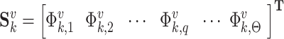
Residue-level analysis

The task of residue-level analysis can be generally described as follows. Given a dataset containing I sequences with N residues, in order to predict the attributes of the residues, each residue should be classified into one of the M categories, where each category is composed of residues with the same attribute, and its size is. Evidently, the total number of samples is. The uth residue in is expressed by

(2)

where is the pth feature of the uth residue in category m.

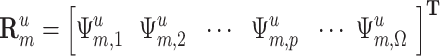
Sequence-level analysis

Given a dataset containing I sequences (see Equation 1) from K categories, where each category is composed of sequences with the same attribute, and its size is. The total number of sequence samples is. The vth sequence in category is expressed by (56)

(3)

where is the qth feature of the vth sequence in category k.

Now the difficulty is, for a residue or a sequence, how to identify which category it belongs to? To cope with such a problem, we proposed a powerful and multifunctional web server in this study, named BioSeq-Analysis2.0, through which users can construct various sequence-level and residue-level predictors for analyzing DNA, RNA and protein sequences.

BioSeq-Analysis2.0 updates the three sub web servers (DNA-Analysis2.0, RNA-Analysis2.0, Protein-Analysis2.0) for analyzing DNA, RNA and protein sequences, respectively. Each of them is able to automatically implement the three main steps: feature extraction, predictor construction and performance evaluation (see Figure 1).

Feature extraction

The residue-level features explore the properties of the residues, and their relationship among the residues in the sliding windows, while the sequence-level features focus on extracting the global information along the entire sequences. For residue-level analysis, in order to capture the properties of the residues, the sliding window strategy and the fragment strategy were used to extract the corresponding features via a user defined fixed-length window. For sequence-level analysis, the biological sequences (see Equation 1) were converted into feature vectors via sequence information. BioSeq-Analysis2.0 for the first time provides 26 features for residue-level analysis. BioSeq-Analysis2.0 updates 34 new features at sequence level, leading to 90 features for sequence-level analysis. In this section, we mainly focused on introducing the 26 features for residue-level analysis and the 34 new features for sequence-level analysis. For the other 56 features for sequence-level analysis, please refer to (1).

In DNA-Analysis2.0, there are seven different residue-level features for DNA sequences to generate various predictors, which can be further divided into three categories (Table 1).

Table 1.

Seven residue-level features for DNA sequences

Category	Feature	Description
Residue composition	One-hot	Basic one-hot (17)
	Position-specific-2	Position-specific of two nucleotides (18)
	Position-specific-3	Position-specific of three nucleotides (18)
	Position-specific-4	Position-specific of four nucleotides (18)
Physicochemical property	DPC	Dinucleotide physicochemical (19,20)
	TPC	Trinucleotide physicochemical (19)
Evolutionary information	BLAST-matrix	BLAST-matrix (21)

The first category is about residue composition containing four features. Of the four, the first one is of One-hot, where the residues are arranged in a particular order, and then the ith residue type is represented by four binary bits with the ith bit set as 1, and all the other bits are set as 0; the rest of the four are Position-specific-2 (18), Position-specific-3 (18) and Position-specific-4 (18), reflecting different position specificity between any two nucleotides along a DNA sequence based on One-hot.

The second category is about physicochemical property containing two features, DPC and TPC. The former (DPC) is based on the 90 physicochemical indices of dinucleotides extracted from (19,20) to represent residues, while the latter depends on 12 physicochemical properties of trinucleotides extracted from (19) to represent residues. Both the two features can select some physicochemical indices from the built-in index boxes.

The third category is about evolutionary information containing one feature BLAST-matrix based on (21), which can represent the local and global DNA sequence composition.

In RNA-Analysis2.0, there are six different residue-level features for RNA sequences to generate various predictors, which can be separated into three categories (Table 2)

Table 2.

Six residue-level features for RNA sequences

Category	Feature	Description
Residue composition	One-hot	Basic one-hot (17)
	Position-specific-2	Position-specific of two nucleotides (18)
	Position-specific-3	Position-specific of three nucleotides (18)
	Position-specific-4	Position-specific of four nucleotides (18)
Physicochemical property	DPC	Dinucleotide physicochemical (19)
Structure composition	SS	Secondary structure (22)

The first category is about residue composition containing four features. Three of the four are Position-specific-2 (18), Position-specific-3 (18) and Position-specific-4 (18), reflecting different position specificity between any two nucleotides along a RNA sequence based on One-hot. The last one of the four is basic One-hot.

The second category is about physicochemical property containing one feature, DPC, which represents residues depended on the 11 physicochemical properties of dinucleotides extracted from (19). Users can select physicochemical indices from the built-in index boxes.

The third category is about structure composition containing one feature SS, which represents the secondary structure of each residue extracted from (22), therefore, SS can represent the local RNA structure composition.

In Protein-Analysis2.0, there are 13 different residue-level features for protein sequences to generate various predictors, which can be further divided into the following four categories (Table 3)

Table 3.

Thirteen residue-level features for protein sequences

Category	Feature	Description
Residue composition	One-hot	Basic one-hot (17)
	One-hot(6-bit)	6-dimension One-hot method (23)
	Binary(5-bit)	Use five binary bit to encode (24)
	AESNN3	Learn from alignments (25)
	Position-specific-2	Position-specific of two residues (18)
Physicochemical property	PP	Properties form AAindex (26)
Structure composition	SS	Secondary structure (27)
	SASA	Solvent accessible surface area (28)
Evolutionary information	PAM250	PAM250 matrix (29)
	BLOSUM62	BLOSUM62 matrix (30)
	PSSM	PSSM matrix (31)
	PSFM	Frequency profiles matrix (11)
	CS	Conservation score (32)

The first category is about residue composition containing five features. Of the five, the first one is One-hot, the dimension of each residue is 20. The next two features One-hot (6-bit) (23) and Binary (5-bit) (24) are to reduce the dimension and complexity of One-hot. The fourth feature is Position-specific-2 based on One-hot to represent the local protein sequence composition, and the fifth feature is AESNN3 (25) based on the characteristics generated by machine learning techniques.

The second category is PP that represents residues using the 547 amino acid physicochemical indices from AAindex (26), and users can select some physicochemical properties from the index boxes to use.

The third category is about structure composition containing two features: SS (27), and SASA (28) based on secondary structure and relative solvent accessibility information of each residue, respectively.

The fourth category is about evolutionary information that containing five features: PAM250 (29), BLOSUM62 (30), PSSM (31), PSFM (11), and CS (32). Of the five features, PAM250 is based on the homologous protein sequences, and BLOSUM62 is based on the BLOCKS database of aligned protein sequences. Both the PSSM and PSFM features are based on sequence alignments, which were generated by using PSI-BLAST searching against the NRDB90 database with num_iter of 3, evalue_threshold of 0.0001, and num_threads of 40. The CS is based on sequence conservation score.

Please note that nine new sequence-level features in the nucleotide acid composition category for DNA/RNA were added (Table 4), including multiple nucleic acid composition, nucleotide chemical property, Electron-ion interaction pseudopotentials of trinucleotide for DNA. Eighteen new sequence-level features for proteins were added (Table 5) into the three categories: amino acid composition, autocorrelation, predicted structure features.

Table 4.

Nine new sequence-level features for DNA/RNA sequences.

Category	Feature	Type	Description
Nucleotide acid composition	NAC	DNA/RNA	Nucleic Acid Composition (2)
	DNC	DNA/RNA	Di-Nucleotide Composition (2)
	TNC	DNA/RNA	Tri-Nucleotide Composition (2)
	CKSNAP	DNA/RNA	Composition of k-spaced Nucleic Acid Pairs (2)
	NCP	DNA/RNA	Nucleotide Chemical Property (2)
	ANF	DNA/RNA	Accumulated Nucleotide Frequency (33)
	Zcurve	DNA/RNA	Representation of DNA/RNA sequence (35)
	EIIP	DNA	Electron-ion interaction pseudopotentials of trinucleotide only for DNA (34)
	PseEIIP	DNA	Electron-ion interaction pseudopotentials of trinucleotide only for DNA (2)

Table 5.

Eighteen new sequence-level features for protein sequences

Category	Feature	Description
Amino acid composition	AAC	Amino Acid Composition (37)
	GAAC	Grouped Amino Acid Composition (38)
	CTDC	Composition (C), transition (T), and distribution (D) (39)
	CTDT	Composition (C), transition (T), and distribution (D) (39,40)
	CTDD	Composition (C), transition (T), and distribution (D) (39,40)
	CTriad	Conjoint Triad (41)
	SOCNumber	Sequence-Order-Coupling Number (42)
	QSOrder	Quasi-sequence-order (43)
	Z-Scale	ZSCALE (44,45)
	TPC	Tri-Peptide Composition (37)
	GTPC	Grouped Tri-Peptide Composition (37)
	CKSAAP	Composition of k-spaced Amino Acid Pairs (46–49)
	CKSAAGP	Composition of k-Spaced Amino Acid Group Pairs (46–49)
	PAAC	Pseudo-Amino Acid Composition (50,51)
Autocorrelation	MAC	Moran autocorrelation (52,53)
	GAC	Geary autocorrelation (54)
	NMMAC	Normalized Moreau-Broto Autocorrelation (53)
Predicted structure features	SSEB	Secondary Structure Binary (55)

Since the dimension of some feature extraction methods is tremendously high, which will result in high-dimension disaster (57).To cope with this problem, in BioSeq-Analysis2.0, users can reduce the feature vector dimension into a user-defined length by using mutual information (58) or chi-square algorithm (59). The chi-square feature selection qualitatively measures the correlation of independent features only for classification purpose. Mutual information is the amount of information of one feature contained in another feature. The chi-square test makes it easier to give high scores for features occurring less frequently. For example, if a feature appears once in the benchmark dataset, it will get a relatively high score, while its mutual information score will be low.

Predictor construction

Most of biological sequence analysis tasks at residue level and sequence level can be treated as classification tasks. Therefore, many classifiers have been applied to biological sequence analysis.

For residue-level analysis, BioSeq-Analysis2.0 incorporates two classification algorithms (Support Vector Machine (SVM) (60), Random Forest (RF) (61)), and a sequence labelling algorithm (Conditional Random Fields (CRF) (62)).

For SVM algorithm, its implementation was depended on the LIBSVM package (63) with the kernel of Gaussian radial basis function (RBF), and users can select the values of the c and g (c is from to , g is from to ) or these parameters can be automatically optimized according to specific performance measures, such as accuracy (Acc), Matthew's correlation coefficient (MCC) or area under ROC (64) curve (AUC) (64). RF is a flexible and widely used supervised machine learning algorithm. The Python Scikit-learn (65) package was used as its implementation in BioSeq-Analysis2.0, and the users can select the value of n_estimators (the number of the decision trees, whose range is from 100 to 800). This parameter can also be automatically optimized.

Furthermore, in order to capture the global and long-range sequence order information of residues, a sequence labelling algorithm Conditional Random Field (CRF) (62) was provided for residue-level analysis. Compared with the transitional classification classifiers, such as SVM and RF, CRF is a sequence labelling algorithm that is able to model the biological sequences in a global fashion considering the dependency information of all the residues along the sequences as shown in Figure 2. DNA, RNA, or protein sequences are treated as observation sequences, and each residue in the sequences is labeled as 0 or 1. Given the biological sequences X and their labels Y, a conditional probability model can be trained with X and Y. For each observation sequence x, the conditional probability for its label sequence y can be calculated by (62):

(4)

where is a normalization factor, represents a transition feature function (66) about observation sequence x and labels at position i-1 and i. represents a state feature function about observation sequence x and the label at position i. The index k of and the index l of is the number of different feature extraction methods. and are the weights of and , respectively.

Figure 2.

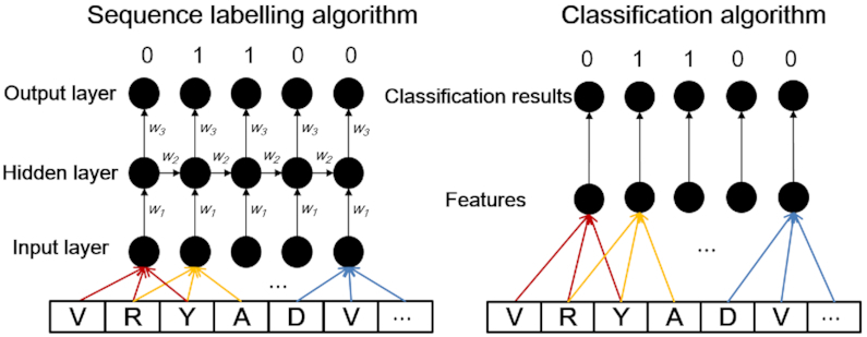
The relationship between sequence labelling algorithm and classification algorithm. Compared with the classification algorithm, the sequence labelling algorithm is able to consider the interactions among residues along the sequence in a global fashion.

For residue-level analysis, the FlexCRFs (http://flexcrfs.sourceforge.net/documents.html (accessed on June 2019)) toolkit was used as the implementation of CRF, which was modified to deal with the real value features following this study (67). The parameters of the num_iterations (the number of training iterations) and the init_lambda_val (the initial value for the feature weights) were set as 50 and 0.05, respectively.

For sequence-level analysis, four classification algorithms were employed in BioSeq-Analysis2.0. For more details, please refer to (1).

Performance evaluation

According to the aforementioned two processes, a predictor for analyzing biological sequence tasks can be generated. Evaluating performance of the predictor is an important component (68). In BioSeq-Analysis2.0, two methods are used for realizing this purpose, containing 5-fold cross-validation and independent test.

In 5-fold cross-validation, the benchmark dataset is randomly partitioned into five roughly equivalent subsets. The training procedure is repeated five times with different training and test sets. Please note that in order to avoid overestimating the performance of the residue-level predictors, all the residues in one sequence must be in the same subset, which is different from the sequence-level analysis. Besides 5-fold cross-validation, the independent test is usually adopted to evaluate a predictor of the real world applications. The predictor is trained with the benchmark dataset, and tested on the independent dataset. The independent dataset should be fully independent from the benchmark dataset so as to fairly evaluate its performance.

The training sets are often imbalanced for some biological sequence analysis tasks, for example, for the protein disordered region prediction task, the number of the residues in the ordered regions is much larger than the number of residues in the disordered regions (66), which will inevitably lead to a bias consequence (66). In this regard, the oversampling and under sampling techniques were also provided to minimize this bias consequence in BioSeq-Analysis2.0.

In BioSeq-Analysis2.0, five metrics were used to measure the predictor's quality for binary classification tasks, including Sn, Sp, Acc, MCC and AUC, calculated by (8,69):

(5)

where and represent the total amount of positive samples and the total amount of negative samples, respectively. Whereas represents the amount of positive samples wrongly predicted as negative samples and represents the amount of the negative samples wrongly predicted as positive samples.

For multiclass classification tasks, Acc was used to evaluate the performance, calculated by (6):

(6)

where represents the total amount of the samples in the ith class, whereas is the amount of the samples in the ith class wrongly predicted as the other classes and represents the total amount of the samples not in the ith class, whereas is the amount of the samples not in the ith class wrongly predicted to be the ith class.

RESULTS AND DISCUSSION

Web server

BioSeq-Analysis2.0 is an updated platform for analyzing DNA, RNA, and protein sequences at sequence level and residue level based on machine learning approaches. The pipeline of BioSeq-Analysis2.0 is shown in Figure 3.

Figure 3.

The pipeline of the web server of BioSeq-Analysis 2.0.

Input

The input page of BioSeq-Analysis2.0 web server is shown in Figure 4. The input sequences should be in FASTA format, which can be written into the input box, or uploaded as a separate file. For residue-level analysis tasks, the corresponding label for each residue should be given. For DNA-Analysis2.0, 7 and 29 DNA feature extraction methods at residue level and sequence level respectively are provided. For RNA-Analysis2.0, 6 and 21 RNA feature extraction methods at residue-level and sequence-level respectively are provided. For Protein-Analysis2.0, 13 and 40 protein feature extraction methods at residue-level and sequence-level respectively are provided. The users should select one feature from the above features. For residue-level analysis, the fragment method or the size of the sliding window should be selected. Two feature selection methods (mutual information or chi-square algorithm) can be used to select representative features so as to avoid the high dimension disaster. The next step is to choose one operation engine. The parameters of the feature extraction methods and the machine learning classifiers can be automatically optimized. Furthermore, the oversampling and under sampling techniques can be used to handle the imbalanced training set problem.

Figure 4.

A screenshot to show that BioSeq-Analysis2.0 contains three sub servers, including (i) DNA-Analysis2.0, (ii) RNA-Analysis2.0, (iii) Protein-Analysis2.0 for residue-level analysis (A) and sequence-level analysis (B). For each of the three sub-servers, users can generate their desired predictors via the buttons marked with (iv), (v) and (vi).

Output

Figure 5 is a result page using One-hot feature in the sub web server DNA-Analysis2.0 with the provided example data (sliding window size 7, c, and g =) as the input.

Figure 5.

A screenshot to show the result page of DNA-Analysis2.0. It contains six panels: (A) the parameter summary, including the input sequence type, selected feature, and the selected machine learning algorithm; (B) the 5-fold cross-validation results, including Acc, MCC, AUC, Sn, and Sp; (C) the generated ROC curve; (D) the trained model with parameters; (E) features in Scikit-learn format; (F) features in Weka format.

Figure 5A includes two parts. The first part is the parameters of the selected feature containing feature name and the size of the sliding window, and the other part is the parameters of the selected machine learning algorithm such as the value of c, and g. Figure 5B shows the 5-fold cross-validation evaluation results, which is a table listing the values of Acc, MCC, AUC, Sn, and Sp to evaluate the performance of the DNA-Analysis2.0. Figure 5C is the ROC curve generated by the DNA-Analysis2.0, which has good robustness to the distribution of positive and negative samples. Figure 5D is an example output of the trained model that can be directly downloaded for further analysis. The trained model includes the total number of the categories (nr_class), the number of support vectors (total_sv) and the number of support vectors for each category (nr_sv), the parameters of the machine learning algorithm (gamma), etc. Figure 5E shows an example output of the generated features in Scikit-learn format, for convenience, it can be downloaded directly as a separate file. For the stand-alone package, the output file format can be chosen from the tab-delimited format, LIBSVM format, and the CSV format, which will be used for further computational analysis. Figure 5F gives an example output of generated features in Weka format containing three parts: relation, attribute and data, which can also be downloaded directly as a separate file. Relation is the relationship name of the dataset, and attribute is an attribute description for each sample in the dataset.

Stand-alone package of BioSeq-Analysis2.0

In order to deal with the biological sequence analysis tasks with large datasets, the stand-alone package of BioSeq-Analysis2.0 web server is also provided, which can be accessed at http://bliulab.net/BioSeq-Analysis2.0/download. There are two main modules in the BioSeq-Analysis2.0 stand-alone package for residue level analysis, one is feature extraction module with five executive python scripts: ‘ei.py’, ‘ssc.py’, ‘rc.py’, ‘pp.py’ and ‘feature.py’, the other module is ‘train.py’ and ‘rf_method.py’ for predictor construction and performance evaluation. For the convenience of the user, the processes of feature extraction, predictor construction and performance evaluation were combined into one executive python scripts ‘analysis.py’. There are also some scripts that help users to find the best predictor for a specific biological sequence analysis task. Please refer to the user manual for more details. Additionally, the multiprocessing technique was employed to further reduce the computing time of this stand-alone package.

Applications of BioSeq-Analysis2.0

In this section, BioSeq-Analysis2.0 stand-alone package was applied to three important residue-level biological sequence analysis tasks, including protein disordered region prediction (66), enhancer prediction (8), and mRNA N6-methyladenosine (m⁶A) site prediction (6).

The predictors for these tasks can be easily generated using BioSeq-Analysis2.0. Particularly, the performance of some predictors automatically generated by BioSeq-Analysis2.0 is highly comparable or even better than the existing predictors, indicating that BioSeq-Analysis2.0 is a powerful tool for generating new predictors for analysing biological sequence tasks.

Identification of enhancers

Enhancer is short DNA region that can be bound by proteins (activators) to activate a gene transcription (7). Therefore, the identification of enhancers is important for studying the transcription process, which can be treated as a binary classification task. In this study, the DNA-Analysis2.0 was used to generate 14 different predictors for enhancer prediction based on the 7 residue-level feature extraction methods for DNA sequences (Table 1), and two machine learning algorithms: SVM and RF. Each predictor can be easily generated by running the following command line:

python analysis.py sequence_file DNA –method feature_extraction_method –ml machine_learning_method –labels label_file –fragment 1 –model model_name

Evaluated on a widely used benchmark dataset (7,8), the ROC curves of the 14 predictors were listed in Figure 6, from which we can see that the SVM-One-hot predictor achieves the top performance with an AUC score of 0.8267, even outperforming the existing approach reported in (70), indicating that BioSeq-Analysis2.0 is useful for generating new predictors for enhancer identification.

Figure 6.

An illustration of the ROC curves and the values of AUC of 14 different predictors for the identification of enhancers generated by DNA-Analysis2.0 on the benchmark dataset (7,8) based on SVM (A) and RF (B).

Identification of mRNAs (m6A) sites

N6-Methyladenosine (m⁶A) is an RNA methylation modification at the nitrogen-6 position of the adenosine base (6). Research in cancer biology has shown that m⁶A mRNA modification plays a critical role in glioblastoma stem cell self-renewal and tumorigenesis (71,72). Therefore, the identification of the m⁶A becomes a hot topic.

In this study, the RNA-Analysis2.0 in BioSeq-Analysis2.0 was used to generate 12 different predictors for mRNAs (m⁶A) site prediction based on the 6 residue-level feature extraction methods (Table 2), and two machine learning algorithms: SVM and RF. Each predictor can be easily generated by running the following command line:

python analysis.py sequence_file RNA –method feature_extraction_method –ml machine_learning_method –labels label_file –fragment 1 –model model_name

Figure 7 shows the ROC curves of the 12 predictors automatically generated by BioSeq-Analysis2.0. These experimental results further confirmed that RNA-Analysis2.0 was useful for developing new predictors for RNA sequence analysis tasks as well.

Figure 7.

An illustration of the ROC curves and the values of AUC of 12 different predictors for mRNAs (m⁶A) site identification generated by RNA-Analysis2.0 on the subset of the benchmark dataset (6) based on SVM (A) and RF (B).

Identification of protein disordered regions

Intrinsically disordered proteins lack stable three dimensional structures in their native states (66), which are correlated with many diseases, such as genetic diseases, cancer, etc. Therefore, identification of disordered proteins and regions has become one of the most popular tasks in the studies of protein structures and functions (66,69). Here, Protein-Analysis2.0 in BioSeq-Analysis2.0 was used to automatically generate various predictors for protein disordered region prediction based on the benchmark dataset (66). Finally, 26 predictors were generated based on the 13 residue-level feature extraction methods of proteins (see Table 3), and two machine learning algorithms: CRF and SVM. Each predictor can be easily generated by running the following command line:

python analysis.py sequence_file Protein –method feature_extraction_method –ml machine_learning_method –labels label_file –model model_name –size sliding_window_size

The ROC curves of the 26 predictors were shown in Figure 8, where we can see that the feature extraction methods and machine learning algorithms impact on the performance of the corresponding predictors, and the predictors based on the sequence labeling model CRFs generally outperformed those based on the SVM, which is fully consistent with a recent study (66). Particularly, the CRF-One-hot (6-bit) predictor can achieve an AUC score of 0.7472, highly comparable with the existing state-of-the-art methods in this filed (66).

Figure 8.

An illustration of the ROC curves and the values of AUC of 26 different predictors for disordered protein identification generated by Protein-Analysis2.0 on the subset of the benchmark dataset (66) based on CRF (A) and SVM (B).

As shown in some recent studies, machine learning techniques are playing more and more important roles in biological sequence analysis (73,74), such as protein remote homology detection (75), protein fold recognition (76), etc. It can be anticipated that the proposed BioSeq-Analysis2.0 will become a very useful tool for the researchers who are interested in developing new computational predictors for these tasks.

Notes

Present address: Bin Liu, Beijing Institute of Technology, No. 5, South Zhongguancun Street, Haidian District, Beijing 100081, China.

FUNDING

National Natural Science Foundation of China [61822306]; Fok Ying-Tung Education Foundation for Young Teachers in the Higher Education Institutions of China [161063]; Scientific Research Foundation in Shenzhen [JCYJ20180306172207178]. Funding for open access charge: National Natural Science Foundation of China [61822306].

Conflict of interest statement. None declared.

REFERENCES

- 1. Liu B. BioSeq-Analysis: a platform for DNA, RNA and protein sequence analysis based on machine learning approaches. Brief. Bioinform. 2017; doi:10.1093/bib/bbx165. [DOI] [PubMed] [Google Scholar]
- 2. Chen Z., Zhao P., Li F., Marquez-Lago T.T., Leier A., Revote J., Zhu Y., Powell D.R., Akutsu T., Webb G.I. et al.. iLearn: an integrated platform and meta-learner for feature engineering, machine-learning analysis and modeling of DNA, RNA and protein sequence data. Brief. Bioinform. 2019; doi:10.1093/bib/bbz041. [DOI] [PubMed] [Google Scholar]
- 3. Wei L., Hu J., Li F., Song J., Su R., Zou Q.. Comparative analysis and prediction of quorum-sensing peptides using feature representation learning and machine learning algorithms. Brief. Bioinform. 2018; doi:10.1093/bib/bby107. [DOI] [PubMed] [Google Scholar]
- 4. Bock J.R., Gough D.A.. Predicting protein–protein interactions from primary structure. Bioinformatics. 2001; 17:455–460. [DOI] [PubMed] [Google Scholar]
- 5. Ishida T., Kinoshita K.. PrDOS: prediction of disordered protein regions from amino acid sequence. Nucleic Acids Res. 2007; 35:W460–W464. [DOI] [PMC free article] [PubMed] [Google Scholar]
- 6. Zou Q. Sr., Xing P., Wei L., Liu B.. Gene2vec: gene subsequence embedding for prediction of mammalian N6-methyladenosine sites from mRNA. RNA. 2018; 25:205–218. [DOI] [PMC free article] [PubMed] [Google Scholar]
- 7. Liu B., Fang L.Y., Long R., Lan X., Chou K.C.. iEnhancer-2L: a two-layer predictor for identifying enhancers and their strength by pseudo k-tuple nucleotide composition. Bioinformatics. 2016; 32:362–369. [DOI] [PubMed] [Google Scholar]
- 8. Liu B., Li K., Huang D.S., Chou K.C.. iEnhancer-EL: identifying enhancers and their strength with ensemble learning approach. Bioinformatics. 2018; 34:3835–3842. [DOI] [PubMed] [Google Scholar]
- 9. Chen J.J., Guo M.Y., Wang X.L., Liu B.. A comprehensive review and comparison of different computational methods for protein remote homology detection. Brief. Bioinform. 2018; 19:231–244. [DOI] [PubMed] [Google Scholar]
- 10. Yan K., Xu Y., Fang X.Z., Zheng C.H., Liu B.. Protein fold recognition based on sparse representation based classification. Artif. Intell. Med. 2017; 79:1–8. [DOI] [PubMed] [Google Scholar]
- 11. Liu B., Zhang D.Y., Xu R.F., Xu J.H., Wang X.L., Chen Q.C., Dong Q.W., Chou K.C.. Combining evolutionary information extracted from frequency profiles with sequence-based kernels for protein remote homology detection. Bioinformatics. 2014; 30:472–479. [DOI] [PMC free article] [PubMed] [Google Scholar]
- 12. Chen J.J., Guo M.Y., Li S.M., Liu B.. ProtDec-LTR2.0: an improved method for protein remote homology detection by combining pseudo protein and supervised Learning to Rank. Bioinformatics. 2017; 33:3473–3476. [DOI] [PubMed] [Google Scholar]
- 13. Liu B., Wang X., Zou Q., Dong Q., Chen Q.. Protein Remote Homology Detection by Combining Chou's Pseudo Amino Acid Composition and Profile-Based Protein Representation. Mol. Inf. 2013; 32:775–782. [DOI] [PubMed] [Google Scholar]
- 14. Liu B., Wang S., Long R., Chou K.-C.. iRSpot-EL: identify recombination spots with an ensemble learning approach. Bioinformatics. 2017; 33:35–41. [DOI] [PubMed] [Google Scholar]
- 15. Yan J., Friedrich S., Kurgan L.. A comprehensive comparative review of sequence-based predictors of DNA- and RNA-binding residues. Brief. Bioinform. 2016; 17:88–105. [DOI] [PubMed] [Google Scholar]
- 16. Zhang J., Liu B.. PSFM-DBT: identifying DNA-binding proteins by combing position specific frequency matrix and distance-Bigram transformation. Int. J. Mol. Sci. 2017; 18:E1856. [DOI] [PMC free article] [PubMed] [Google Scholar]
- 17. Yoo P.D., Zhou B.B., Zomaya A.Y.. Machine learning techniques for protein secondary structure prediction: an overview and evaluation. Curr. Bioinform. 2008; 3:74–86. [Google Scholar]
- 18. Doench J.G., Fusi N., Sullender M., Hegde M., Vaimberg E.W., Donovan K.F., Smith I., Tothova Z., Wilen C., Orchard R. et al.. Optimized sgRNA design to maximize activity and minimize off-target effects of CRISPR-Cas9. Nat. Biotechnol. 2016; 34:184–191. [DOI] [PMC free article] [PubMed] [Google Scholar]
- 19. Chen W., Zhang X.T., Brooker J., Lin H., Zhang L.Q., Chou K.C.. PseKNC-General: a cross-platform package for generating various modes of pseudo nucleotide compositions. Bioinformatics. 2015; 31:119–120. [DOI] [PubMed] [Google Scholar]
- 20. Friedel M., Nikolajewa S., Suhnel J., Wilhelm T.. DiProDB: a database for dinucleotide properties. Nucleic Acids Res. 2009; 37:D37–D40. [DOI] [PMC free article] [PubMed] [Google Scholar]
- 21. Altschul S., Madden T., Schaffer A., Zhang J.H., Zhang Z., Miller W., Lipman D.. Gapped BLAST and PSI-BLAST: a new generation of protein database search programs. FASEB J. 1998; 12:A1326–A1326. [DOI] [PMC free article] [PubMed] [Google Scholar]
- 22. Hofacker I.L., Fontana W., Stadler P.F., Bonhoeffer L.S., Tacker M., Schuster P.. Fast folding and comparison of RNA secondary structures. Monatsh. Chem. 1994; 125:167–188. [Google Scholar]
- 23. Wang J.T.L., Ma Q., Shasha D., Wu C.H.. New techniques for extracting features from protein sequences. IBM Syst. J. 2001; 40:426–441. [Google Scholar]
- 24. White G., Seffens W.. Using a neural network to backtranslate amino acid sequences. Electron. J. Biotechnol. 1998; 1:17–18. [Google Scholar]
- 25. Lin K., May A.C.W., Taylor W.R.. Amino acid encoding schemes from protein structure alignments: multi-dimensional vectors to describe residue types. J. Theor. Biol. 2002; 216:361–365. [DOI] [PubMed] [Google Scholar]
- 26. Kawashima S., Pokarowski P., Pokarowska M., Kolinski A., Katayama T., Kanehisa M.. AAindex: amino acid index database, progress report 2008. Nucleic Acids Res. 2008; 36:D202–D205. [DOI] [PMC free article] [PubMed] [Google Scholar]
- 27. Cuff J.A., Barton G.J.. Application of multiple sequence alignment profiles to improve protein secondary structure prediction. Proteins. 2000; 40:502–511. [DOI] [PubMed] [Google Scholar]
- 28. Heffernan R., Paliwal K., Lyons J., Dehzangi A., Sharma A., Wang J., Sattar A., Yang Y., Zhou Y.. Improving prediction of secondary structure, local backbone angles, and solvent accessible surface area of proteins by iterative deep learning. Sci. Rep. 2015; 5:11476. [DOI] [PMC free article] [PubMed] [Google Scholar]
- 29. MO D. A model of evolutionary change in proteins. Atlas Protein Seq. Struct. 1978; 5:89–99. [Google Scholar]
- 30. Henikoff S., Henikoff J.G.. Amino-acid substitution matrices from protein blocks. P Natl Acad Sci USA. 1992; 89:10915–10919. [DOI] [PMC free article] [PubMed] [Google Scholar]
- 31. Altschul S.F., Koonin E.V.. Iterated profile searches with PSI-BLAST - a tool for discovery in protein databases. Trends Biochem. Sci. 1998; 23:444–447. [DOI] [PubMed] [Google Scholar]
- 32. Glaser F., Rosenberg Y., Kessel A., Pupko T., Ben-Tal N.. The ConSurf-HSSP database: The mapping of evolutionary conservation among homologs onto PDB structures. Proteins-Struct. Funct. Bioinform. 2005; 58:610–617. [DOI] [PubMed] [Google Scholar]
- 33. Chen W., Tran H., Liang Z., Lin H., Zhang L.J. Sr. Identification and analysis of the N 6-methyladenosine in the Saccharomyces cerevisiae transcriptome. Sci. Rep. 2015; 5:13859. [DOI] [PMC free article] [PubMed] [Google Scholar]
- 34. Nair A.S., Sreenadhan S.P.J.B.. A coding measure scheme employing electron-ion interaction pseudopotential (EIIP). Bioinformation. 2006; 1:197–202. [PMC free article] [PubMed] [Google Scholar]
- 35. Gao F., Zhang C.T.. Comparison of various algorithms for recognizing short coding sequences of human genes. Bioinformatics. 2004; 20:673–U232. [DOI] [PubMed] [Google Scholar]
- 36. Liu Y., Wang X., Liu B.. A comprehensive review and comparison of existing computational methods for intrinsically disordered protein and region prediction. Brief. Bioinform. 2017; 20:330–346. [DOI] [PubMed] [Google Scholar]
- 37. Bhasin M., Raghava G.P.J.J.O.B.C.. Classification of nuclear receptors based on amino acid composition and dipeptide composition. J. Biol. Chem. 2004; 279:23262–23266. [DOI] [PubMed] [Google Scholar]
- 38. Lee T.-Y., Lin Z.-Q., Hsieh S.-J., Bretaña N.A., Lu C.-T.J.B.. Exploiting maximal dependence decomposition to identify conserved motifs from a group of aligned signal sequences. Bioinformatics. 2011; 27:1780–1787. [DOI] [PubMed] [Google Scholar]
- 39. Dubchak I., Muchnik I., Holbrook S.R., Kim S.-H.J.P.O.T.N.A.O.S.. Prediction of protein folding class using global description of amino acid sequence. Proc. Natl. Acad. Sci. U.S.A. 1995; 92:8700–8704. [DOI] [PMC free article] [PubMed] [Google Scholar]
- 40. Dubchak I., Muchnik I., Mayor C., Dralyuk I., Kim S.H.J.P.S.. Recognition of a protein fold in the context of the SCOP classification. Proteins. 1999; 35:401–407. [PubMed] [Google Scholar]
- 41. Shen J., Zhang J., Luo X., Zhu W., Yu K., Chen K., Li Y., Jiang H.J.P.O.T.N.A.O.S.. Predicting protein–protein interactions based only on sequences information. Proc. Natl. Acad. Sci. U.S.A. 2007; 104:4337–4341. [DOI] [PMC free article] [PubMed] [Google Scholar]
- 42. Chou K.C., Cai Y.D.J.J.O.C.B. Prediction and classification of protein subcellular location—sequence‐order effect and pseudo amino acid composition. J. Cell. Biochem. 2003; 90:1250–1260. [DOI] [PubMed] [Google Scholar]
- 43. Chou K.-C.J.B. Prediction of protein subcellular locations by incorporating quasi-sequence-order effect. Biochem Biophys Res Commun. 2000; 278:477–483. [DOI] [PubMed] [Google Scholar]
- 44. Sandberg M., Eriksson L., Jonsson J., Sjöström M., Wold S.J.J.O.M.C. New chemical descriptors relevant for the design of biologically active peptides. A multivariate characterization of 87 amino acids. J. Med. Chem. 1998; 41:2481–2491. [DOI] [PubMed] [Google Scholar]
- 45. Chen Y.-Z., Chen Z., Gong Y.-A., Ying G.J.P.O.. SUMOhydro: a novel method for the prediction of sumoylation sites based on hydrophobic properties. PLoS One. 2012; 7:e39195. [DOI] [PMC free article] [PubMed] [Google Scholar]
- 46. Chen K., Jiang Y., Du L., Kurgan L.J.J.O.C.C. Prediction of integral membrane protein type by collocated hydrophobic amino acid pairs. J. Comput. Chem. 2009; 30:163–172. [DOI] [PubMed] [Google Scholar]
- 47. Chen K., Kurgan L., Rahbari M.J.B.. Prediction of protein crystallization using collocation of amino acid pairs. Biochem. Biophys. Res. Commun. 2007; 355:764–769. [DOI] [PubMed] [Google Scholar]
- 48. Chen K., Kurgan L.A., Ruan J.J.B.s.b. Prediction of flexible/rigid regions from protein sequences using k-spaced amino acid pairs. BMC Struct. Biol. 2007; 7:25. [DOI] [PMC free article] [PubMed] [Google Scholar]
- 49. Chen K., Kurgan L.A., Ruan J.J.J.O.C.C. Prediction of protein structural class using novel evolutionary collocation‐based sequence representation. J Comput. Chem. 2008; 29:1596–1604. [DOI] [PubMed] [Google Scholar]
- 50. Chou K.C.J.P.S. Prediction of protein cellular attributes using pseudo‐amino acid composition. Proteins Struct. Funct. Bioinform. 2001; 43:246–255. [DOI] [PubMed] [Google Scholar]
- 51. Chou K.-C.J.B. Using amphiphilic pseudo amino acid composition to predict enzyme subfamily classes. Bioinformatics. 2004; 21:10–19. [DOI] [PubMed] [Google Scholar]
- 52. Feng Z.-P., Zhang C.-T.. Prediction of membrane protein types based on the hydrophobic index of amino acids. J. Protein Chem. 2000; 19:269–275. [DOI] [PubMed] [Google Scholar]
- 53. Horne D.S. Prediction of protein helix content from an autocorrelation analysis of sequence hydrophobicities. Biopolymers. 1988; 27:451–477. [DOI] [PubMed] [Google Scholar]
- 54. Sokal R.R., Thomson B.A.. Population structure inferred by local spatial autocorrelation: an example from an Amerindian tribal population. Am. J. Phys. Anthropol. 2006; 129:121–131. [DOI] [PubMed] [Google Scholar]
- 55. Sun S., Thomas P.D., Dill K.A.J.P.E.. A simple protein folding algorithm using a binary code and secondary structure constraints. Protein. Eng. 1995; 8:769–778. [DOI] [PubMed] [Google Scholar]
- 56. Chou K.C. Some remarks on protein attribute prediction and pseudo amino acid composition. J. Theor. Biol. 2011; 273:236–247. [DOI] [PMC free article] [PubMed] [Google Scholar]
- 57. Lin H., Deng E.Z., Ding H., Chen W., Chou K.C.. iPro54-PseKNC: a sequence-based predictor for identifying sigma-54 promoters in prokaryote with pseudo k-tuple nucleotide composition. Nucleic Acids Res. 2014; 42:12961–12972. [DOI] [PMC free article] [PubMed] [Google Scholar]
- 58. Ross B.C. Mutual Information between Discrete and Continuous Data Sets. PLoS One. 2014; 9:e87357. [DOI] [PMC free article] [PubMed] [Google Scholar]
- 59. Liu B., Wang X.L., Lin L., Dong Q.W., Wang X.. A discriminative method for protein remote homology detection and fold recognition combining Top-n-grams and latent semantic analysis. BMC Bioinformatics. 2008; 9:510. [DOI] [PMC free article] [PubMed] [Google Scholar]
- 60. Suykens J.A.K., Vandewalle J.. Least squares support vector machine classifiers. Neural Process Lett. 1999; 9:293–300. [Google Scholar]
- 61. Ho T.K. The random subspace method for constructing decision forests. IEEE Trans. Pattern Anal. 1998; 20:832–844. [Google Scholar]
- 62. Lafferty J., Mccallum A., Pereira F.. Conditional Random Fields: Probabilistic Models for Segmenting and Labeling Sequence Data. Proc. ICML. 2001; 3:282–289. [Google Scholar]
- 63. Chang C.C., Lin C.J.. LIBSVM: A Library for Support Vector Machines. ACM Trans. Intel. Syst. Tech. 2011; 2:27:1–27:27. [Google Scholar]
- 64. Fawcett T. An introduction to ROC analysis. Pattern Recogn. Lett. 2006; 27:861–874. [Google Scholar]
- 65. Pedregosa F., Varoquaux G., Gramfort A., Michel V., Thirion B., Grisel O., Blondel M., Prettenhofer P., Weiss R., Dubourg V. et al.. Scikit-learn: machine learning in python. J. Mach. Learn. Res. 2011; 12:2825–2830. [Google Scholar]
- 66. Liu Y., Wang X., Liu B.. IDP-CRF: intrinsically disordered protein/region identification based on conditional random fields. Int. J. Mol. Sci. 2018; 19:E2483. [DOI] [PMC free article] [PubMed] [Google Scholar]
- 67. Li M.H., Lin L., Wang X.L., Liu T.. Protein-protein interaction site prediction based on conditional random fields. Bioinformatics. 2007; 23:597–604. [DOI] [PubMed] [Google Scholar]
- 68. Liu B., Li C., Yan K.. DeepSVM-fold: protein fold recognition by combining support vector machines and pairwise sequence similarity scores generated by deep learning networks. Brief. Bioinform. doi:10.1093/bib/bbz098. [DOI] [PubMed] [Google Scholar]
- 69. Liu B., Xu J.H., Lan X., Xu R.F., Zhou J.Y., Wang X.L., Chou K.C.. iDNA-Prot vertical bar dis: identifying DNA-binding proteins by incorporating amino acid distance-pairs and reduced alphabet profile into the general pseudo amino acid composition. PLoS One. 2014; 9:e106691. [DOI] [PMC free article] [PubMed] [Google Scholar]
- 70. Jia C., He W.. EnhancerPred: a predictor for discovering enhancers based on the combination and selection of multiple features. Sci. Rep. 2016; 6:38741. [DOI] [PMC free article] [PubMed] [Google Scholar]
- 71. Cui Q., Shi H., Ye P., Li L., Qu Q., Sun G., Sun G., Lu Z., Huang Y., Yang C.G. et al.. m(6)A RNA methylation regulates the self-renewal and tumorigenesis of glioblastoma stem cells. Cell Rep. 2017; 18:2622–2634. [DOI] [PMC free article] [PubMed] [Google Scholar]
- 72. Zhang S., Zhao B.S., Zhou A., Lin K., Zheng S., Lu Z., Chen Y., Sulman E.P., Xie K., Bogler O. et al.. m(6)A demethylase ALKBH5 maintains tumorigenicity of glioblastoma stem-like cells by sustaining FOXM1 expression and cell proliferation program. Cancer Cell. 2017; 31:591–606. [DOI] [PMC free article] [PubMed] [Google Scholar]
- 73. Liu B., Liu F., Wang X., Chen J., Fang L., Chou K.-C.. Pse-in-One: a web server for generating various modes of pseudo components of DNA, RNA, and protein sequences. Nucleic Acids Res. 2015; 43:W65–W71. [DOI] [PMC free article] [PubMed] [Google Scholar]
- 74. Wu Z., Liao Q., Liu B.. A comprehensive review and evaluation of computational methods for identifying protein complexes from protein-protein interaction networks. Brief. Bioinform. doi:10.1093/bib/bbz085. [DOI] [PubMed] [Google Scholar]
- 75. Liu B., Zhu Y.. ProtDec-LTR3.0: protein remote homology detection by incorporating profile-based features into learning to rank. IEEE ACCESS. 2019; 7:102499–102507. [Google Scholar]
- 76. Yan K., Fang X., Xu Y., Liu B.. Protein fold recognition based on multi-view modeling. Bioinformatics. 2019; doi:10.1093/bioinformatics/btz040. [DOI] [PubMed] [Google Scholar]