A Utility Approach to Individualized Optimal Dose Selection Using Biomarkers

Abstract

In many settings, including oncology, increasing the dose of treatment results in both increased efficacy and toxicity. With the increasing availability of validated biomarkers and prediction models, there is the potential for individualized dosing based on patient specific factors. We consider the setting where there is an existing dataset of patients treated with heterogenous doses and including binary efficacy and toxicity outcomes and patient factors such as clinical features and biomarkers. The goal is to analyze the data to estimate an optimal dose for each (future) patient based on their clinical features and biomarkers. We propose an optimal individualized dose finding rule by maximizing utility functions for individual patients while limiting the rate of toxicity. The utility is defined as a weighted combination of efficacy and toxicity probabilities. This approach maximizes overall efficacy at a prespecified constraint on overall toxicity. We model the binary efficacy and toxicity outcomes using logistic regression with dose, biomarkers and dose-biomarker interactions. To incorporate the large number of potential parameters, we use the LASSO method. We additionally constrain the dose effect to be non-negative for both efficacy and toxicity for all patients. Simulation studies show that the utility approach combined with any of the modeling methods can improve efficacy without increasing toxicity relative to fixed dosing. The proposed methods are illustrated using a dataset of patients with lung cancer treated with radiation therapy.

1. Introduction

The goal of personalized medicine is to give the right treatment to the right patient at the right dose using all we know about the patient. Available knowledge about individual patients is increasingly including biomarkers which allow personalizing treatment decisions. One approach to personalized medicine is to identify the right patient for a given treatment. For example, in the setting of a single binary outcome and two potential treatments, Foster et. al (2011) proposed a “Virtual Twins” method involving predicting response probabilities for treatment and control “twins” for each subject by random forest, and then using regression or classification trees to identify subgroups of patients with large positive treatment effect estimates. A related but different approach is to identify the right treatment for a patient, often referred to as optimal treatment regimes (OTR). A treatment regime is defined as the function that maps a patient’s covariate vector to one of the treatment choices. One approach to identify an OTR is a 2-step method that involves building a model for conditional expectation of the outcome given treatment as the first step, then maximizing the mean expected reward to get the optimal treatment for each subject. In an alternative approach, rather than modeling the marginal outcome, outcome weighted learning (OWL) methods maximize the reward from following a treatment regime directly, which is equal to the expected outcome in a subset of patients who actually followed that regime, inversely weighted by the probability of being assigned to the regime (Zhao et al., 2012). Maximizing the reward with respect to the treatment regime is equivalent to minimizing the expectation for patients who did not follow the regime, and can be interpreted as minimizing the weighted classification error in a classification problem (Zhang et al., 2012a). Zhang et. al (2012b) also proposed the doubly robust augmented inverse probability weighted estimator (AIPWE) in which an outcome model is combined with a model for the probability of a treatment which is important when analyzing observational data. The OWL method has been extended to continuous treatment dose settings such as optimal dose finding (Chen et al., 2016).

In many settings, it is not possible to describe a patient’s outcome using a single variable. For example, in oncology, it is typical to describe patient outcomes in terms of toxicity and efficacy variables. Several strategies have been proposed for identifying an optimal treatment or dose based on the trade-off between efficacy and toxicity. Thall and Cook (2004) proposed using efficacy-toxicity trade-off contours that partition the two-dimensional outcome probability domain such that efficacy-toxicity pairs on the same contour are equally desirable. Dose could then be selected to maximize desirability. More commonly, a utility matrix is elicited from clinicians by assigning numerical utilities to each possible bivariate outcome. The optimal dose is then defined as the value maximizing the posterior mean utility (Guo and Yuan, 2017).

Guo and Yuan (2017) proposed a Phase I/II trial design incorporating biomarkers in which the optimal dose for an individual patient is selected to maximize utility. A joint model of ordinal toxicity and efficacy outcomes is specified and canonical partial least squares are used to extract a small number of components from the covariate matrix containing dose, biomarkers, and dose-by-biomarker interactions. Wang et. al (2018) proposed two approaches to identify a personalized optimal treatment strategy that maximizes clinical benefit under a constraint on the average risk in the situation of a binary treatment option and continuous outcomes.

In this paper we propose a utility based method to estimate optimal doses for individual patients in the setting of binary efficacy and toxicity outcomes. To allow for potentially large numbers of biomarkers and patient factors we utilize l₁-penalty via LASSO (Tibshirani, 1996). At the individual level, we find the optimal dose by maximizing utility functions defined as the probability of efficacy minus the weighted probability of toxicity, which is equivalent to a utility matrix (Schipper et al., 2014). The weight term in the utility equation could be elicited from clinicians to quantify the relative undesirability of toxicity relative to lack of efficacy. Alternatively it can be viewed as a tuning parameter selected to achieve a desired overall (at the population level) rate of toxicity. In the vast majority of oncology treatments and many other disease settings, both efficacy and toxicity outcomes are monotonically linked to increasing dose. While “flat” curves are common (Postel-Vinay et al., 2009), it is uncommon for increasing dose to lead to decreased toxicity or efficacy. We note that monotonicity may not hold for outcomes such as progression free survival which include death as an event, since they are potentially a consequence of either toxicity or lack of efficacy. When estimating outcomes as a function of dose only it is often not necessary to impose this constraint. However, when including many potential dose*biomarker interactions, it is likely that some patients will be estimated to have decreasing toxicity or efficacy with increasing dose due to statistical noise. To prevent this and to improve efficiency we propose a method that constrains the estimated dose-efficacy and dose-toxicity relationships to be non-decreasing for all patients. We call this constrained LASSO, which can be solved by decomposition and quadratic programming (He, 2011) and alternating direction method of multipliers (ADMM) (Gains and Zhou, 2016). In section 3, we report results of a simulation study and in section 4 we illustrate the proposed methods using a dataset of patients with lung cancer treated with radiation therapy.

2. Method

2.1. Binary Outcome Setting

We assume the available data, (x_i, d_i, E_i, T_i), i = 1, …, n, comprises n independent and identically distributed copies of (x, d, E, T), where x, a p-dimensional centered vector of subject-specific features, d ∈ [−1, 1] denotes continuous dose of treatment, E is the binary efficacy outcome, and T is the binary toxicity outcome. A large probability of E and small probability of T is preferable.

An individualized dose rule is the map from x to the dose domain: $\mathcal{F}:{\mathbb{R}}^p\to [-1,1]$. Under $\mathcal{F}$, a patient with covariate x is recommended to dose $d=\mathcal{F}(x)$. For any treatment rule $\mathcal{F}$, the population expected efficacy and toxicity are ${\mathbb{E}}^{\mathcal{F}}(E)$ and ${\mathbb{E}}^{\mathcal{F}}(T)$. Our goal is to estimate an individualized dose rule that maximizes the population expected efficacy while controlling the overall expected toxicity under some tolerance level, that is

$${\max }_{\mathcal{F}}{\mathbb{E}}^{\mathcal{F}}(E),\text{subject to}{\mathbb{E}}^{\mathcal{F}}(T)\le \tau ,$$ (1)

where τ is the pre-specified maximal tolerance level of average toxicity.

Define δ_E(x_i, d_i) =P(E = 1∣d_i, x_i)−P(E = 1∣d_i = −1, x_i), δ_T(x_i, d_i) =P(T = 1∣d_i, x_i)−P(T = 1∣d_i = −1, x_i). δ_E(x_i, d_i) and δ_T(x_i, d_i) can be interpreted as the difference in expected efficacy and toxicity outcomes for a patient if treated at the lowest dose (d_i = −1) or some higher dose (d_i). Let ${\mathbb{E}}_x$ to denote the population average of the function across the distribution of x. After introducing the Lagrange multiplier, solving equation (1) is equivalent to

$${\max }_{\mathcal{F}}{\mathbb{E}}_x[{\delta }_E\{x_i,\mathcal{F}(x_i)\}-\theta {\delta }_T\{x_i,\mathcal{F}(x_i)\}],$$ (2)

where θ > 0 is chosen such that ${\mathbb{E}}_x[{\delta }_T\{x_i,\mathcal{F}(x_i)\}]\le \tau -{\mathbb{E}}_x[\mathrm{P}(T=1\mid d_i=-1,x_i)]$. The expression in equation (2) is a utility function quantifying the trade-off between efficacy and toxicity. By fitting separate models for E and T using methods such as logistic regression via maximum likelihood or constrained LASSO as described below, we can calculate the utility values for individual patients over the range of possible dose values, and calculate the dose rule that maximizes equation (2).

Consider the model logit{P(Y = 1)} = f(x, d, β) = β₀ + Wβ between outcome Y, i.e. E or T, and covariates including biomarkers x, dose d, and dose-biomarker interactions dx, i.e. W = (x, d, dx). To fit the model we use the generalized LASSO with l₁-penalty on the log-likelihood and no penalty on β₀. To enforce a non-decreasing relationship of efficacy and toxicity with dose, we add constraints on derivatives with respect to d to be non-negative, i.e., $\frac{\partial }{\partial d}f(x_i,d,\beta )\ge 0$ for all x_i. We call this method constrained LASSO (cLASSO), for which the constraint can be written as Cβ ≥ 0, where C is a n × (2p + 1) matrix of [$0_{n\ast p},1_{n\ast 1},{\mathit{x}}_{n\ast p}$]. Then the cLASSO method is to

$$\text{minimize}-\log L(\beta ,W,Y)+\lambda \Vert \beta {\Vert }_1=-\sum _{i=1}^n[Y_i({\beta }_0+W_i\beta )-\log \{1+\text{exp}({\beta }_0+W_i\beta )\}]+\lambda \Vert \beta {\Vert }_1$$ (3)

subject to Cβ ≥ 0.

To solve (3) we decompose β into its positive and negative part, β = β⁺ − β⁻, as the relation ∣β∣ = β⁺ + β⁻ handles the l₁ penalty term. Let W * = (W, −W), and β* = (β^+T, −β^−T)^T. By plugging these into (3) and adding the additional non-negativity constraints on β⁺ and β⁻, the constrained LASSO is formulated and can be solved, for example, by spg() in R, which uses the spectral projected gradient method for large-scale optimization with simple constraints. That is,

$$\text{minimize}-\sum _{i=1}^n[Y_i({\beta }_0+W_i^{\ast }{\beta }^{\ast })-\log \{1+\text{exp}({\beta }_0+W_i^{\ast }{\beta }^{\ast })\}]+\lambda {1_{4p+2}}^T{\beta }^{\ast }$$ (4)

subject to (C, −C)β* ≥ 0, β⁺ ≥ 0, β⁻ ≥ 0.

The derivative of (4) with respect to (β₀, β*) is

$$-\sum _{i=1}^n\{Y_i(1,W_i^{\ast })-\frac{\text{exp}({\beta }_0+W_i^{\ast }{\beta }^{\ast })}{1+\text{exp}({\beta }_0+W_i^{\ast }{\beta }^{\ast })}(1,W_i^{\ast })\}+\lambda (0,{1_{4p+2}}^T)$$ (5)

The minimizer to (4) always satisfies ${\beta }_j^{+}{\beta }_j^{-}=0$ for j = 1, …, 2p + 1, as shown in the Appendix. We use 10-fold cross-validation(CV) to choose λ to minimize the CV deviance.

For any fixed value of theta, and using the above estimated models of efficacy and toxicity, we can find the optimal dose for each patient that maximize (2), then we use grid search to find the smallest θ achieving the constraint on toxicity. Specifically the algorithm is as follows:

1. Set a grid 0 = θ₁ < θ₂ < … < θ_K

2. For each m =1, …, K:

   1. set θ = θ_m
   2. For each subject i = 1, …, n with covariate x_i: calculate $d_i^{opt}=\text{argmax}({\delta }_E(x_i,d)-\theta {\delta }_T(x_i,d))$, estimate $\mathrm{P}(E=1\mid d_i^{opt},x_i)$ and $\mathrm{P}(T=1\mid d_i^{opt},x_i)$

3. Select the smallest $\widehat{\theta }$ such that ${\mathbb{E}}_x[\mathrm{P}(T=1\mid d_i^{opt}(\theta ),x_i)]\le \tau$. Then $d_i^{opt}(\widehat{\theta })$ is the estimated optimal dose for patient i.

For binary outcomes under the logistic link function, both δ_E(x, d) and δ_T(x, d) are functions involving the intercept, main effect of x, as well as dose related covariates d and dx. Estimation of d^opt at given θ for each subject is solved by one-dimensional optimization using optimize() in R, which uses a combination of golden section search and successive parabolic interpolation. Because of the non-decreasing dose-efficacy and dose-toxicity relationship, a larger θ will recommend a smaller d^opt, and the corresponding population average efficacy and toxicity will be smaller. So the smallest θ achieving the constraint on average toxicity will achieve the largest average efficacy. The range and size of the grid can be pre-specified and should include a range of feasible values. In our simulation and data example, we used a range of 0.01 to 4, in steps of 0.001. We note that for the determination of $d_i^{opt}$, we consider the subject level E − T trade-off, while for the determination of θ, we look at the population level E − T trade-off.

2.2. Multiple Outcome Setting

In some applications there are multiple toxicity outcomes which must be considered and balanced against efficacy when selecting treatment dose. Without loss of generality, we consider two different toxicity outcomes T₁, T₂ and the goal is to

$${\max }_{\mathcal{F}}{\mathbb{E}}^{\mathcal{F}}(E),\text{subject to}{\mathbb{E}}^{\mathcal{F}}(T_1)\le {\tau }_1,{\mathbb{E}}^{\mathcal{F}}(T_2)\le {\tau }_2$$ (6)

where τ₁, τ₂ are the pre-specified maximal tolerance levels of average toxicity for each toxicity outcome.

Define δ_E(x_i, d_i) =P(E = 1∣d_i, x_i)−P(E = 1∣d_i = −1, x) δ_T1(x_i, d_i) =P(T₁ = 1∣d_i, x_i)−P(T₁ = 1∣d_i = −1, x_i), δ_T2(x_i, d_i) =P(T₂ = 1∣d_i, x_i)−P(T₂ = 1∣d_i = −1, x_i). Then equation (6) is equivalent to

$${\max }_{\mathcal{F}}{\mathbb{E}}_x[{\delta }_E\{x_i,\mathcal{F}(x_i)\}-{\theta }_1{\delta }_{T_1}\{x_i,\mathcal{F}(x_i)\}-{\theta }_2{\delta }_{T_2}\{x_i,\mathcal{F}(x_i)\}],$$ (7)

where θ₁ > 0, θ₂ > 0 are chosen such that ${\mathbb{E}}_x[{\delta }_{T_1}\{x_i,\mathcal{F}(x_i)\}]\le {\tau }_1-{\mathbb{E}}_x[\mathrm{P}(T_1=1\mid d_i=-1,x_i)]$, and ${\mathbb{E}}_x[{\delta }_{T_2}\{x_i,\mathcal{F}(x_i)\}]\le {\tau }_2-{\mathbb{E}}_x[\mathrm{P}(T_2=1\mid d_i=-1,x_i)]$.

We specify parametric logistic models for E, T₁, T₂ as functions of biomarkers, dose, and dose-biomarker interactions. Denote the parameter estimates from those logistic models as ${\widehat{\beta }}_E$, ${\widehat{\beta }}_{T_1}$, ${\widehat{\beta }}_{T_2}$. We propose a random walk and Metropolis algorithm to select θ₁, θ₂ to achieve the constraints on toxicity. The algorithm is as follows:

1. Set a chain length, B, fix σ² > 0 and initialize ${\theta }^0=({\theta }_1^0,{\theta }_2^0)$ to a starting value that makes ${\mathbb{E}}_x[\mathrm{P}(T_1=1\mid d_i^{opt}({\theta }^0),x_i)]\le {\tau }_1$, ${\mathbb{E}}_x[\mathrm{P}(T_2=1\mid d_i^{opt}({\theta }^0),x_i)]\le {\tau }_2$.

2. For b = 0, …, B:

   1. Generate ${\tilde{\theta }}^{b+1}\sim N({\theta }^b,{\sigma }^2\mathit{I})$ and ${\tilde{\theta }}^{b+1}>0$
   2. For each subject i = 1, …, n with covariate x_i: compute $d_i^{opt}=\text{arg}\max \{{\delta }_E(x_i,d)-{\tilde{\theta }}_1^{b+1}{\delta }_{T_1}(x_i,d)-{\tilde{\theta }}_2^{b+1}{\delta }_{T_2}(x_i,d)\}$, estimate $\mathrm{P}(E=1\mid d_i^{opt}({\tilde{\theta }}^{b+1}),x_i)$, $\mathrm{P}(T_1=1\mid d_i^{opt}({\tilde{\theta }}^{b+1}),x_i)$, and $\mathrm{P}(T_2=1\mid d_i^{opt}({\tilde{\theta }}^{b+1}),x_i)$
   3. Compute $q=\text{min}[1,{\mathbb{E}}_x\{\mathrm{P}(E=1\mid d_i^{opt}({\tilde{\theta }}^{b+1}),x_i)\}∕{\mathbb{E}}_x\{Pr(E=1\mid d_i^{opt}({\theta }^b),x_i)\}]$
   4. Generate U ~ U(0, 1); if ${\mathbb{E}}_x[\mathrm{P}(T_1=1\mid d_i^{opt}({\tilde{\theta }}^{b+1}),x_i)]\le {\tau }_1$, ${\mathbb{E}}_x[\mathrm{P}(T_2=1\mid d_i^{opt}({\tilde{\theta }}^{b+1}),x_i)]\le {\tau }_2$, and U ≤ q, set ${\theta }^{b+1}={\tilde{\theta }}^{b+1}$ otherwise, set θ^b+1 = θ^b

3. After generating a chain (θ⁰, …, θ^B), we select the θ^k that leads to the largest value of ${\mathbb{E}}_x[\mathrm{P}(E=1\mid d_i^{opt}({\theta }^k),x_i)]$ as the optimal solution, and the $d_i^{opt}({\theta }^k)$ is the optimal dose for patient i.

In stage 2(b) in the above algorithm, d^opt at given θ for each subject is solved by one-dimensional optimization using optimize() in R. The variance of the proposal distribution σ² in stage 2(a) is chosen to make the acceptance proportion between 0.25 and 0.5. When there are multiple constraints we found that the random walk and Metropolis algorithm is more efficient than using a finite grid search over the multiple dimensions of θ. In our experience, as long as the chain is long enough, the maxima of the population average efficacy will be achieved. This can be checked by running the algorithm in parallel for different initial choices of θ⁰. It is noted that there is no guarantee that both toxicity constraints will be met at the boundary.

3. Simulation Studies

In this section, we performed numerical studies to investigate the performance of the proposed method under different settings. We simulated five i.i.d covariates, x₁, …, x₅ from a standard normal distribution, d from Uniform(−1, 1), and then generated N=200 binary outcomes E and T from the regression models

$$\log \text{it}(\mathrm{P}(E=1))={\beta }_{0,E}+W_E{\beta }_E,$$

$$\log \text{it}(\mathrm{P}(T=1))={\beta }_{0,T}+W_T{\beta }_T,$$

where W_E = W_T = (x, d, dx). A range of scenarios for β were considered, but we first describe scenario 0, as given in Table 1. For scenario 0 (β_0,E, β_E) =(0, 1, 0, 0, 0, 0, 1, .4, .4, .4, −.8, 0), and (β_0,T, β_T) =(−1.386, −1, 0, 0, 0, 0, 1, −.4, −.4, −.4, .8, 0). In generating x’s, we also applied the constraints that x must satisfy 1 + 0.4x₁ + 0.4x₂ + 0.4x₃ − 0.8x₄ > 0 and 1 − 0.4x₁ − 0.4x₂ − 0.4x₃ + 0.8x₄ > 0 to reflect the non-decreasing dose-efficacy and dose-toxicity curves for all subjects. This excludes up to 35% of the originally simulated observations.

Table 1:

Simulation results. Summary of average Efficacy improvement compared with fixed dose with P(Toxicity) constrained to be ≤ 0.2. Results from 1000 simulated trials. Each scenario true logistic models for E and T include main effect for the biomarkers, dose and biomarker-dose interactions, with coefficients as shown below.

Scenarios	Efficacy and Toxicity model coefficients												FS	LASSO	cLASSO	Possible Improvement	cLASSO > LASSO
		Biomarker					Dose	Interactions
0	E	1	0	0	0	0	1	.4	.4	.4	−.8	0	0.513	0.518	0.589	0.147	69.0%
	T	−1	0	0	0	0	1	−.4	−.4	−.4	.8	0
1	E	1	0	0	0	0	1	0	0	0	0	0	0.393	0.659	0.694	0.052	53.3%
	T	−1	0	0	0	0	1	0	0	0	0	0
2	E	1	0	0	0	0	1	.4	.4	.4	−.8	0	0.344	0.340	0.375	0.070	56.7%
	T	−1	0	0	0	0	1	.4	.4	.4	−.8	0
3	E	1	0	0	0	0	1	.4	.4	.4	−.8	0	0.216	0.332	0.354	0.146	60.4%
	T	−1	0	0	0	0	1	−.4	−.4	−.4	.8	0
4	E	1	0	0	0	0	1	.4	.4	.4	−.8	0	NA	0.246	0.272	0.146	60.0%
	T	−1	0	0	0	0	1	−.4	−.4	−.4	.8	0
5	E	1	0	0	0	0	1	.4	.4	.4	−.8	0	0.692	0.691	0.762	0.148	71.7%
	T	−1	0	0	0	0	1	−.4	−.4	−.4	.8	0
6	E	1	0	0	0	0	1	.4	.4	.4	−.8	0	0.433	0.431	0.461	0.148	66.3%
	T	−1	0	0	0	0	1	−.4	−.4	−.4	.8	0
7	E	1	0	0	0	0	1	.4	.4	.4	−.8	0	0.561	0.561	0.628	0.147	66.2%
	T	−1	0	0	0	0	1	−.4	−.4	−.4	.8	0
8	E	1	0	0	0	0	1	.4	.4	.4	−.8	0	0.378	0.399	0.450	0.200	58.2%
	T	−1	0	0	0	0	1	−.4	−.4	−.4	.8	0
9	E	1	0	0	0	0	1	.4	.4	.4	−.8	0	0.360	0.402	0.481	0.206	64.6%
	T	−1	0	0	0	0	1	−.4	−.4	−.4	.8	0
10	E	1	0	0	0	0	1	.4	.4	.4	−.8	0	0.455	0.466	0.551	0.146	69.3%
	T	−1	0	0	0	0	1	−.4	−.4	−.4	.8	0
0*	E	1	.2	.3	.1	0	1	0	.2	−.1	.6	0	0.618	0.648	0.694	0.132	62.9%
	T	−1	−.2	−.3	−.1	0	1	0	−.2	.1	−.6	0
1*	E	1	.2	.3	.1	0	1	0	0	0	0	0	0.410	0.590	0.641	0.055	56.4%
	T	−1	−.2	−.3	−.1	0	1	0	0	0	0	0
2*	E	1	.2	.3	.1	0	1	0	.2	−.1	.6	0	0.373	0.497	0.647	0.053	77.5%
	T	−1	−.2	−.3	−.1	0	1	0	.2	−.1	.6	0
3*	E	1	.2	.3	.1	0	1	0	.2	−.1	.6	0	0.280	0.429	0.460	0.131	62.1%
	T	−1	−.2	−.3	−.1	0	1	0	−.2	.1	−.6	0
4*	E	1	.2	.3	.1	0	1	0	.2	−.1	.6	0	NA	0.307	0.342	0.133	61.7%
	T	−1	−.2	−.3	−.1	0	1	0	−.2	.1	−.6	0
5*	E	1	.2	.3	.1	0	1	0	.2	−.1	.6	0	0.788	0.802	0.833	0.134	64.0%
	T	−1	−.2	−.3	−.1	0	1	0	−.2	.1	−.6	0
6*	E	1	.2	.3	.1	0	1	0	.2	−.1	.6	0	0.512	0.613	0.640	0.133	62.0%
	T	−1	−.2	−.3	−.1	0	1	0	−.2	.1	−.6	0
7*	E	1	.2	.3	.1	0	1	0	.2	−.1	.6	0	0.671	0.716	0.756	0.134	65.0%
	T	−1	−.2	−.3	−.1	0	1	0	−.2	.1	−.6	0
8*	E	1	.2	.3	.1	0	1	0	.2	−.1	.6	0	0.391	0.435	0.457	0.153	54.8%
	T	−1	−.2	−.3	−.1	0	1	0	−.2	.1	−.6	0
9*	E	1	.2	.3	.1	0	1	0	.2	−.1	.6	0	0.317	0.372	0.435	0.081	65.6%
	T	−1	−.2	−.3	−.1	0	1	0	−.2	.1	−.6	0
10*	E	1	.2	.3	.1	0	1	0	.2	−.1	.6	0	0.519	0.559	0.624	0.132	68.4%
	T	−1	−.2	−.3	−.1	0	1	0	−.2	.1	−.6	0

^a.The intercept for Efficacy models is 0, for Toxicity models is −1.386.

^b.Possible $\text{Improvement}={\mathbb{E}}^{{\mathcal{F}}_{Theory}}(E)-{\mathbb{E}}^{{\mathcal{F}}_{FD}}(E)$, the percentage of $\text{improvement}=\{{\mathbb{E}}^{\mathcal{F}}(E)-{\mathbb{E}}^{{\mathcal{F}}_{FD}}(E)\}∕\{{\mathbb{E}}^{{\mathcal{F}}_{Theory}}(E)-{\mathbb{E}}^{{\mathcal{F}}_{FD}}(E)\}$.

^c.Scenarios 3, 6, 3*, 6* have 15 noise covariates with coefficients 0 added; scenarios 4, 4* have 45 noise covariates with coefficients 0 added.

^d.Scenarios 5, 6, 5*, 6* have doubled sample size of 400.

^e.Scenario 7, 7* have cor(x₁, x₂, x₃) = 0.6.

^f.Scenarios 8, 9, 10, 8*, 9*, 10* have mis-specified models.

In scenario 8, 8*, the true effect of covariate x₄ is stepwise at 0, e.g.,logit(P(E = 1)) = x₁ + d + (0.4x₁ + 0.4x₂ + 0.4x₃ − 0.8I(x₄ > 0))d.

In scenario 9, 9*, the true models have exp(x₄) as the covariate,e.g.,logit(P(E = 1)) = x₁ + d +(0.4x₁ + 0.4x₂+ 0.4x₃ − 0.8exp(x₄))d.

In scenario 10, 10*, an interaction of x₂ and x₃ is included as main effect in both true models for efficacy and toxicity, e.g.,logit(P(E = 1)) = x₁ + x₂x₃ + d + (0.4x₁ + 0.4x₂ + 0.4x₃ − 0.8x₄)d.

To illustrate the utility approach to dose selection, we plotted individual level E-T trade-off for three different subjects in Fig.1 and population level E-T trade-off in Fig.2. Different dose-efficacy and dose-toxicity curves among subjects result in selection of different optimal dose values across θ.

Figure 1.

Top: Individual level E-T plot with choice of dose with theoretical β_E, β_T for three subjects. The utility curve uses θ = 1. Bottom: Individual level optimal dose as a function of θ for the same three subjects.

Figure 2.

Left: Population level E-T plot with choice of θ with theoretical β_E, β_T, Right: Population level E-T trade-off at different toxicity tolerance levels.

For variable selection, we forced the main effect for dose to be selected by removing its associated parameter from the penalty term and only consider the selection of covariates and dose*covariate interactions. The methods we compared are forward selection (FS), regular LASSO, cLASSO and fixed dosing (FD) in which dose only logistic models were fit. FS was implemented by step() in R using AIC as criteria. Regular LASSO was implemented by glmnet() in R with 10-fold CV.

The boxplots in Fig.3 shows the average efficacy from the above methods with the same toxicity constraint, from which we see that cLASSO has higher average efficacy compared to the other methods, especially fixed-dose. We also calculate the theoretical improvement from using the true models which would only be known in a simulation study setting. The improvement, defined as proportion of possible gain compared to the gain from FD to theory, $\{{\mathbb{E}}^{\mathcal{F}}(E)-{\mathbb{E}}^{{\mathcal{F}}_{FD}}(E)\}∕\{{\mathbb{E}}^{{\mathcal{F}}_{Theory}}(E)-{\mathbb{E}}^{{\mathcal{F}}_{FD}}(E)\}$, for FS, regular LASSO, and cLASSO is 0.513, 0.518, 0.589, respectively. cLASSO has higher efficacy than LASSO for 69.0% of the simulated datasets.

Figure 3.

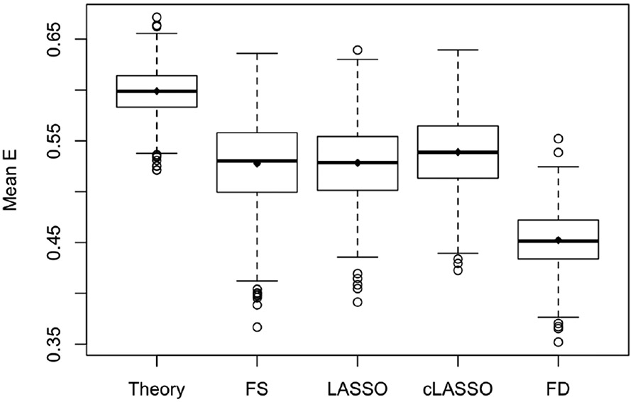
Simulation results for scenario 0. Boxplot of average efficacy with same toxicity for 1000 simulation trials. The compared methods are theory with true coefficients; FS: Forward Selection; LASSO; cLASSO: constrained LASSO; FD: Fixed Dosing. All methods are constrainted at P(T)=0.20. Means are 0.599, 0.528, 0.528, 0.539, 0.452, respectively.

We also considered a null case in which there are no covariates or dose*covariates interactions,so that the dose effects are the same across all subjects. The average efficacy with toxicity constrained at 0.2 for theory, FS, regular LASSO, cLASSO and FD are 0.503, 0.470, 0.490, 0.491, 0.499, respectively. With no effect of covariates, the dose-only model (FD) is as good as the theory, and the models with covariates included have slightly worse performance than the dose-only model. Among the modeling approaches, cLASSO has better performance than FS.

A few other scenarios were considered: In scenario 1 there are only main effects of covariate and no dose-covariate interactions, and the main effects of the same x are in opposite directions in efficacy and toxicity models. In scenario 2, the dose-covariate interaction effects are the same in efficacy and toxicity models, but the main effects of covariates are different. In scenario 3 and 4, there are 15 and 45 additional noise covariates added to increase p from 5 to 20 and 50, to examine the performance with high dimensional data. In scenario 5 and 6, with the same coefficients as in scenario 0 and 3, the sample size increased to 400. In practice, the covariates may be highly correlated resulting in multicollinearity. In scenario 7, x’s are not independent and correlation among x₁, x₂, x₃ are 0.6. We also considered several situations in which the logistic regression model with linear effects is mis-specified. In scenario 8, the true effect of covariate x₄ is stepwise at 0, i.e., the effect only exits for x₄ > 0. But when fitting models, it is mis-specified as linear. In scenario 9, the true models have exp(x₄) as the covariate, but in the fitted models x₄ is used, which is mis-specified. In scenario 10, an interaction of x₂ and x₃ is included as main effect in both true models for efficacy and toxicity, but in the fitted models this interaction is not included.

Table 1 showed the simulation results with the above setting. We also considered another setting with more covariate main effects and fewer dose-covariate interactions, and with the non-decreasing constraints, 12% of the simulated observations were excluded. In scenario 1 and 2, when the dose related coefficients for efficacy and toxicity models are the same or 0, the main effects of covariates still played a role in the optimal dose finding with the logistic link, and cLASSO still has better performance than the other methods. In scenario 3 and 4, with the increased number of noise covariates, the magnitude of improvement decreased, but the cLASSO still performs better than the other methods. In scenario 5 and 6, with the larger sample sizes, the magnitude of improvement increased, and cLASSO outperforms the other methods. In scenario 7, with correlated covariates where the performance of LASSO is known to be suboptimal, cLASSO still performs better than LASSO and FS. In scenario 8, 9, and 10, when the logistic regression model with linear effects is mis-specified, all the methods have smaller magnitude of improvement, but cLASSO still performs better than LASSO and FS, showing the robustness of cLASSO.

In Table A1 in the Supplementary materials we present the results from simulations that considered two toxicity outcomes, T1 and T2. The scenarios were constructed using a subset of the previous efficacy and toxicity models as in Table 1 with toxicity outcome T2 added and constrained at 0.23. The situations considered included a variety of biomarker main effects, dose-biomarker interactions, correlations between the biomarkers and additional noise biomarkers. The results in Table A1 provide similar conclusions regarding the relative merit of cLASSO compared to the other methods as in the single toxicity outcome case.

4. Application

In this section, we applied the proposed method to real data collected from patients with non-small cell lung cancer who received radiation treatment . Patients treated with stereotactic body radiation therapy or with follow-up less than one year were excluded from the analysis, leaving 105 patients in the dataset to be analyzed. Of the 105 patients, 46 had no local, regional or distant progression in two years. Two toxicity outcomes were considered: grade 3+ heart toxicity and grade 3+ lung toxicity. In total, 8 patients had grade 3+ heart toxicity, and 11 patients had grade 3+ lung toxicity that required hospitalization. The clinical features we consider for possible inclusion in models include sex, age, current smoker, Karnofsky Performance Status (KPS), concurrent chemotherapy, simple stage, T-stage, N-stage of the cancer, as shown in Table.2. We also include pre-treatment cytokines level such as interferon γ (IFN-γ), interleukin-1 β (IL-1β), interleukin-2 (IL-2), interleukin-6 (IL-6), tumor necrosis factor α (TNF-α) as prognostic factors. Patients in this study received different doses ranging from 45 Gy to 96 Gy, partially due to the preference of different clinicians as well as the stage of the disease, location of the tumor and the patients performance status. The dose to the tumor site (efficacy dose) is different from the dose received by the lung and heart, but we assume the ratio of them is fixed for each patient. When the optimal efficacy dose is chosen within the observed dose range (45 - 96 Gy), it is multiplied by this known fixed (for each patient) ratio to obtain the lung and heart dose corresponding to the selected tumor dose. There are 14 patients with no cytokine data collected, and multiple imputation with all the covariates and outcomes included is applied to fill in the missing values.

Table 2.

Descriptive statistics of patients (n=105)

Variable	Mean	Range
Age (Years)	65.43	39.60 - 85.20
KPS	85.52	60 - 100
IFN-γ	113.31	0.52 - 6547.50
IL-1β	10.26	0.04 - 92.61
IL-2	23.50	0.04 - 312.22
IL-6	41.93	0.07 - 730.84
TNF-α	18.48	0.54 - 149.37
Tumor dose (Gy)	71.20	45.66 - 96.08
Lung dose (Gy)	14.47	3.17 - 26.11
Heart dose (Gy)	12.22	0.02 - 46.13
Variable	Category	Percentage
Gender	Female	24
	Male	76
Smoking	Current	42
	Never or former	58
chemotherapy	Yes	85
	No	15
Simple stage	1	10
	2	10
	3	79
	4	1
T stage	1	18
	2	23
	3	27
	4	32
N stage	0	23
	1	12
	2	45
	3	20

For the given set of doses in the study, the average probability of no progression in two years (efficacy) is 0.438, the average probability of heart toxicity is 0.076, the average probability of lung toxicity is 0.105, and average tumor dose across patients is 71.20. The goal of this analysis is to estimate an optimal dosing rule that maximize the probability of no progression in 2 years, with heart and lung toxicity level no greater than observed overall toxicity for this population of patients. The efficacy model for the probability of no progression in two years including as covariates the 8 clinical features with their interactions with tumor dose as well as tumor dose has in total 17 possible covariates. The heart toxicity model is built similarly, and the lung toxicity model also includes the 5 most important cytokines and their interaction with lung dose. Table 3 showed the covariates selection by cLASSO in each model. The random walk method of selecting θ ran for 5000 iterations to ensure convergence. With the models built by cLASSO, using the selected optimal dose for each patient gave an expected efficacy of 0.485, an expected heart toxicity at 0.077, an expected lung toxicity at 0.108, and the average tumor dose across patients was 80.21 Gy. With similar expected lung toxicity and heart toxicity rates, the average efficacy increased by 0.047 from 0.438 to 0.485.

Table 3.

Variable selections in each model

Method		cLASSO
Model		Efficacy	Heart toxicity	Lung toxicity
Main effect	Dose	*	*	*
	Age			*
	Sex
	Smoking
	KPS	*	*
	Chemotherapy			*
	S stage
	T stage		*
	N stage	*
	IFN-γ	—	—
	IL-1β	—	—
	IL-2	—	—
	IL-6	—	—
	TNF-α	—	—	*
Interactions with dose	Age	*		*
	Sex			*
	Smoking
	KPS
	Chemotherapy
	S stage
	T stage
	N stage		*
	IFN-γ	—	—
	IL-1β	—	—	*
	IL-2	—	—
	IL-6	—	—
	TNF-α	—	—
Estimated outcomes if these patients were treated at optimal doses		0.485	0.077	0.108

— represents a covariate which is not considered for inclusion in the model.

^*represents a covariate selected by cLASSO for the corresponding model.

Empty cell represent covariates considered for inclusion but not selected by cLASSO.

5. Discussion

In this paper, we propose an optimal individualized dose finding rule by maximizing utility functions for individual patients. This approach maximizes overall efficacy at a prespecified constraint on overall toxicity. We model the binary efficacy and toxicity outcomes using logistic regression with dose, biomarkers and dose-biomarker interactions. To incorporate the larger number of biomarkers and their interaction with doses, we employed the LASSO with linear constraints on the dose related coefficients to constrain the dose effect to be non-negative. Simulation studies show that this approach can improve efficacy without increasing toxicity relative to fixed dosing. Constraining each patient’s estimated dose-efficacy and dose-toxicity curves to be non-decreasing improved performance relative to standard LASSO. This utility method was extended to multiple toxicities.

To force the dose-toxicity or dose-efficacy curve to be non-decreasing with dose, the constraints for linear combination of dose related coefficients only ensure that the patients in the current data satisfy this monotonicity criteria, but monotonicty is not guaranteed for all future patients whose x is not in the observed data. An alternative approach that would ensure monotonicity with respect to dose for all patients would be to force all relevant dose and dose-covariate coefficients to be non-negative. But with the dose-biomarker interactions, it is unnecessary to force all the dose related coefficients to be non-negative, because some of them could be negative but the linear combination of them is non-negative for a selected range of dose and covariate values. Thus, simply constraining all the dose related coefficients to be non-negative is too conservative. It is noted that our method is not appropriate in cases where the toxicity or efficacy endpoint may first increase and then decrease with increasing dose, but is still applicable when there is an increasing effect followed by a plateau.

While we implemented a constrained version of LASSO, other penalized regression approaches such as Elastic Net could also be considered (Zou and Hastie, 2005), or Bayesian methods using Bayesian LASSO (Park and Casella, 2008), or other Bayesian variable selection methods such as “spike-and-slab” (Kuo and Mallick, 1998).

Our method constrains the population averaged toxicity level to be below a given tolerance level. This does not explicitly put any upper bound on the expected toxicity probability for an individual patient. Our method could be modified by including an upper bound on the probability of toxicity for each patient. Thus, in addition to constraints on average toxicity, we also consider adding constraints to individual toxicity, i.e., adding large penalty for extremely high toxicity, which will make the utility function more complex. An indirect way of achieving this would be to use a non-linear function of the probability of toxicity, rather than just the toxicity rate in equation (1).

In this paper we have considered binary outcomes and logistic models that included main effect and dose-biomarker interactions. The method could be generalized to other type of outcomes, such as censored survival times for the efficacy outcome. An ordinal outcome for toxicity could also be accommodated by requiring a different tolerance threshold for each level of toxicity. More flexible forms for the effect of dose and biomarkers could also be considered (e.g., regression splines), and provided the dose monotonicity constraint can be algebraically formulated, the cLASSO would still be applicable.

Appendix A: Proof

The minimizer to problem (4) always satisfies ${\beta }_j^{+}{\beta }_j^{-}=0$ for j = 1,…,2p + 1.

Proof. Proof by contradiction: Consider the minimizer of (4) β = β⁺ + β⁻. Without loss of generality, assume we have ${\beta }_1^{+}>0,{\beta }_1^{-}>0$. Consider another representation of the same $\beta =\stackrel{\stackrel{~}{}}{{\beta }^{+}}-\stackrel{\stackrel{~}{}}{{\beta }^{-}}$.

$$\stackrel{\stackrel{~}{}}{{\beta }_1^{+}}={\beta }_1^{+}-\text{min}({\beta }_1^{+},{\beta }_1^{-}),\stackrel{\stackrel{~}{}}{{\beta }_1^{-}}={\beta }_1^{-}-\text{min}({\beta }_1^{+},{\beta }_1^{-})$$

$$\stackrel{\stackrel{~}{}}{{\beta }_j^{+}}={\beta }_j^{+},\stackrel{\stackrel{~}{}}{{\beta }_j^{-}}={\beta }_j^{-}\text{for}j=2,\dots ,2p+1$$

Obviously, ($\stackrel{\stackrel{~}{}}{{\beta }^{+}}$, $\stackrel{\stackrel{~}{}}{{\beta }^{-}}$) satisfies the constraints of problem (4), and $\stackrel{\stackrel{~}{}}{{\beta }_1^{+}}+\stackrel{\stackrel{~}{}}{{\beta }_1^{-}}<{\beta }_1^{+}+{\beta }_1^{-},\stackrel{\stackrel{~}{}}{{\beta }_1^{+}}-\stackrel{\stackrel{~}{}}{{\beta }_1^{-}}={\beta }_1^{+}-{\beta }_1^{-}$.

Then the objective function (4) can be bounded as L(β⁺, β⁻)

$$\begin{gathered} L({\beta }^{+},{\beta }^{-}) \\ =-\sum \begin{array}{c}n\hfill \\ i=1\hfill \end{array}\left\{y_i({\beta }_0+X_i({\beta }^{+}-{\beta }^{-}))-\log (1+e^{{\beta }_0+X_i({\beta }^{+}-{\beta }^{-})})\right\}+\lambda \sum \begin{array}{c}2p+1\hfill \\ j=1\hfill \end{array}({\beta }^{+}+{\beta }^{-}) \\ =-\sum \begin{array}{c}n\hfill \\ i=1\hfill \end{array}\left\{y_i({\beta }_0+X_i(\stackrel{\stackrel{~}{}}{{\beta }^{+}}-\stackrel{\stackrel{~}{}}{{\beta }^{-}}))-\log (1+e^{{\beta }_0+X_i(\stackrel{\stackrel{~}{}}{{\beta }^{+}}-\stackrel{\stackrel{~}{}}{{\beta }^{-}})})\right\}+\lambda \sum \begin{array}{c}2p+1\hfill \\ j=1\hfill \end{array}({\beta }^{+}+{\beta }^{-}) \\ >-\sum \begin{array}{c}n\hfill \\ i=1\hfill \end{array}\left\{y_i({\beta }_0+X_i(\stackrel{\stackrel{~}{}}{{\beta }^{+}}-\stackrel{\stackrel{~}{}}{{\beta }^{-}}))-\log (1+e^{{\beta }_0+X_i(\stackrel{\stackrel{~}{}}{{\beta }^{+}}-\stackrel{\stackrel{~}{}}{{\beta }^{-}})})\right\}+\lambda \sum \begin{array}{c}2p+1\hfill \\ j=1\hfill \end{array}(\stackrel{\stackrel{~}{}}{{\beta }^{+}}+\stackrel{\stackrel{~}{}}{{\beta }^{-}}) \\ =L(\stackrel{\stackrel{~}{}}{{\beta }^{+}},\stackrel{\stackrel{~}{}}{{\beta }^{-}}). \end{gathered}$$

This contradicts with the assumption that (β⁺, β⁻) is the minimizer of (4).

Appendix B: Additional simulation results

Table A1:

Simulation results for two toxicities. Summary of average Efficacy improvement compared with fixed dose with P(Toxicity1) constrained to be ≤ 0.2 and P(Toxicity2) constrained to be ≤ 0.23. Results from 1000 simulated trials. Each scenario true logistic models for E, T1 and T2 include main effect for the biomarkers, dose and biomarker-dose interactions, with coefficients as shown below.

Scenarios	Efficacy and Toxicity model coefficients												FS	LASSO	cLASSO	Possible Improvement	cLASSO > LASSO
		Biomarker					Dose	Interactions
A0	E	1	0	0	0	0	1	.4	.4	.4	−.8	0	0.581	0.549	0.606	0.121	66.3%
	T1	−1	0	0	0	0	1	−.4	−.4	−.4	.8	0
	T2	−1	0	0	0	0	1	−.5	0	0	0	.5
A1	E	1	0	0	0	0	1	0	0	0	0	0	0.682	0.781	0.800	0.036	50.2%
	T1	−1	0	0	0	0	1	0	0	0	0	0
	T2	−1	0	0	0	0	1	0	0	0	0	0
A2	E	1	0	0	0	0	1	.4	.4	.4	−.8	0	0.639	0.627	0.695	0.114	67.2%
	T1	−1	0	0	0	0	1	−.4	−.4	−.4	.8	0
	T2	−1	0	0	0	0	1	−.5	0	0	0	.5
A3	E	1	0	0	0	0	1	.4	.4	.4	−.8	0	0.454	0.471	0.510	0.121	59.3%
	T1	−1	0	0	0	0	1	−.4	−.4	−.4	.8	0
	T2	−1	0	0	0	0	1	−.5	0	0	0	.5
> o *	E	1	.2	.3	.1	0	1	0	.2	−.1	.6	0	0.659	0.661	0.705	0.111	62.3%
	T1	−1	−.2	−.3	−.1	0	1	0	−.2	.1	−.6	0
	T2	−1	0	0	0	0	1	−.5	0	0	0	.5
A1*	E	1	.2	.3	.1	0	1	0	0	0	0	0	0.575	0.677	0.700	0.039	50.9%
	T1	−1	−.2	−.3	−.1	0	1	0	0	0	0	0
	T2	−1	0	0	0	0	1	0	0	0	0	0
A2*	E	1	.2	.3	.1	0	1	0	.2	−.1	.6	0	0.702	0.667	0.731	0.125	55.1%
	T1	−1	−.2	−.3	−.1	0	1	0	−.2	.1	−.6	0
	T2	−1	0	0	0	0	1	−.5	0	0	0	.5
> CO *	E	1	.2	.3	.1	0	1	0	.2	−.1	.6	0	0.622	0.593	0.658	0.115	60.3 %
	T1	−1	−.2	−.3	−.1	0	1	0	−.2	.1	−.6	0
	T2	−1	0	0	0	0	1	−.5	0	0	0	.5

^a.The intercept for Efficacy models is 0, for Toxicity1 models is −1.386, for Toxicity2 models is −1.2

^b.Possible $\text{Improvement}={\mathbb{E}}^{{\mathcal{F}}_{Theory}}(E)-{\mathbb{E}}^{{\mathcal{F}}_{FD}}(E)$, the percentage of $\text{improvement}=\{{\mathbb{E}}^{\mathcal{F}}(E)-{\mathbb{E}}^{{\mathcal{F}}_{FD}}(E)\}∕\{{\mathbb{E}}^{{\mathcal{F}}_{Theory}}(E)-{\mathbb{E}}^{{\mathcal{F}}_{FD}}(E)\}$.

^c.The random walk method of selecting θ was run for 1000 iterations.

^d. Scenario A2, A2* have cor(x ₁, x₂, x₃) = 0.6.

^e.Scenarios A3, A3* have 15 noise covariates with coefficients 0 added.

References

- Chen G, Zeng D, and Kosorok MR (2016). Personalized dose finding using outcome weighted learning. Journal of the American Statistical Association, 111, 1509–1521. [DOI] [PMC free article] [PubMed] [Google Scholar]
- Foster JC, Taylor JM, and Ruberg SJ (2011). Subgroup identification from randomized clinical trial data. Statistics in Medicine, 30, 2867–2880. [DOI] [PMC free article] [PubMed] [Google Scholar]
- Gaines BR, Kim J, and Zhou H (2018). Algorithms for fitting the constrained lasso. Journal of Computational and Graphical Statistics, 27, 861–871. [DOI] [PMC free article] [PubMed] [Google Scholar]
- Guo B and Yuan Y (2017). Bayesian phase I/II biomarker-based dose finding for precision medicine with molecularly targeted agents. Journal of the American Statistical Association, 112, 508–520. [DOI] [PMC free article] [PubMed] [Google Scholar]
- He T (2011). Lasso and general L1-regularized regression under linear equality and inequality constraints. Unpublished Ph.D. thesis, Purdue University, Dept. of Statistics. [Google Scholar]
- Kuo L and Mallick B (1998). Variable selection for regression models. Sankhyā: The Indian Journal of Statistics, Series B, 65–81. [Google Scholar]
- Park T and Casella G (2008). The Bayesian lasso. Journal of the American Statistical Association, 103, 681–686. [Google Scholar]
- Postel-Vinay S, Arkenau H, Olmos D, Ang J, Barriuso J, Ashley S, Banerji U, De-Bono J, Judson I, and Kaye S (2009). Clinical benefit in phase-I trials of novel molecularly targeted agents: does dose matter? British Journal of Cancer, 100, 1373. [DOI] [PMC free article] [PubMed] [Google Scholar]
- Schipper MJ, Taylor JM, TenHaken R, Matuzak MM, Kong F-M, and Lawrence TS (2014). Personalized dose selection in radiation therapy using statistical models for toxicity and efficacy with dose and biomarkers as covariates. Statistics in Medicine, 33, 5330–5339. [DOI] [PMC free article] [PubMed] [Google Scholar]
- Thall PF and Cook JD (2004). Dose-finding based on efficacy–toxicity trade-offs. Biometrics, 60, 684–693. [DOI] [PubMed] [Google Scholar]
- Tibshirani R (1996). Regression shrinkage and selection via the lasso. Journal of the Royal Statistical Society. Series B (Methodological), 267–288. [Google Scholar]
- Wang Y, Fu H, and Zeng D (2018). Learning optimal personalized treatment rules in consideration of benefit and risk: with an application to treating type 2 diabetes patients with insulin therapies. Journal of the American Statistical Association, 113, 1–13. [DOI] [PMC free article] [PubMed] [Google Scholar]
- Zhang B, Tsiatis AA, Davidian M, Zhang M, and Laber E (2012a). Estimating optimal treatment regimes from a classification perspective. Stat, 1, 103–114. [DOI] [PMC free article] [PubMed] [Google Scholar]
- Zhang B, Tsiatis AA, Laber EB, and Davidian M (2012b). A robust method for estimating optimal treatment regimes. Biometrics, 68, 1010–1018. [DOI] [PMC free article] [PubMed] [Google Scholar]
- Zhao Y, Zeng D, Rush AJ, and Kosorok MR (2012). Estimating individualized treatment rules using outcome weighted learning. Journal of the American Statistical Association, 107, 1106–1118. [DOI] [PMC free article] [PubMed] [Google Scholar]
- Zou H and Hastie T (2005). Regularization and variable selection via the elastic net. Journal of the Royal Statistical Society: Series B (Statistical Methodology), 67, 301–320. [Google Scholar]