An automatic approach to establish clinically desired final dental occlusion for one-piece maxillary orthognathic surgery

Abstract

Purpose

One critical step in routine orthognathic surgery is to reestablish a desired final dental occlusion. Traditionally, the final occlusion is established by hand articulating stone dental models. To date, there are still no effective solutions to establish the final occlusion in computer-aided surgical simulation. In this study, we consider the most common one-piece maxillary orthognathic surgery and propose a three-stage approach to digitally and automatically establish the desired final dental occlusion.

Methods

The process includes three stages: (1) extraction of points of interest and teeth landmarks from a pair of upper and lower dental models; (2) establishment of Midline-Canine-Molar (M-C-M) relationship following the clinical criteria on these three regions; and (3) fine alignment of upper and lower teeth with maximum contacts without breaking the established M-C-M relationship. Our method has been quantitatively and qualitatively validated using 18 pairs of dental models.

Results

Qualitatively, experienced orthodontists assess the algorithm-articulated and hand-articulated occlusions while being blind to the methods used. They agreed that occlusion results of the two methods are equally good. Quantitatively, we measure and compare the distances between selected landmarks on upper and lower teeth for both algorithm-articulated and hand-articulated occlusions. The results showed that there was no statistically significant difference between the algorithm-articulated and hand-articulated occlusions.

Conclusion

The proposed three-stage automatic dental articulation method is able to articulate the digital dental model to the clinically desired final occlusion accurately and efficiently. It allows doctors to completely eliminate the use of stone dental models in the future.

Introduction

In the last decade, computer-aided surgical simulation (CASS) [1, 2] has become a standard of care for orthognathic surgical planning. Orthognathic surgery is specifically designed to correct jaw deformities, and due to the complex nature of the human face, orthognathic surgery requires extensive surgical planning. Using CASS, surgeons are able to plan the entire surgery on the computer.

An important procedure in surgical planning is to establish a desired “final dental occlusion.” The current clinical process is to manually articulate the upper and lower stone dental models together by following the clinical guidelines, i.e., midline alignment, Class I canine relationship, Class I molar relationship, and maximum upper and lower teeth contact, as well as utilizing the instant tactile response to articulate the teeth models. However, unlike in the physical world, the digital teeth models are composed of point clouds which can penetrate into each other regardless of collision between them. For this reason, current CASS planning still requires the traditional dental articulation, in which surgeons are forced to pour the stone models from the dental impression or print the intraorally scanned teeth three-dimensionally, hand-articulate them to the desired final occlusion, and then scan the occluded models together. This is an unnecessary and redundant task, especially when surgeons and orthodontists use an intraoral scanner, which has gained more popularity nowadays and is becoming a standard acquisition tool for dental models.

There are only a few reports on digitally establishing dental occlusion [3–6]. However, these methods, including ours, either require extensive pre-processing or use a haptic feedback device to guide the articulation. Thus, none of them have been successfully utilized in clinical practice.

In this project, we propose a three-stage approach to automatically articulate the dental models to clinical desired final occlusion for routine orthognathic surgery, in which presurgical orthodontic treatment should be completed. The contributions of the proposed method include the following: (1) it utilizes clinical criteria to establish the best possible final dental occlusion as done by surgeons clinically; (2) it is fully automatic and completely eliminates the need for human intervention to generate the digital dental models; and (3) it is computationally efficient. In clinic practice, our approach will ultimately eliminate the need of stone dental models and hand articulation and thus significantly simplify the surgical planning process. A preliminary version of this approach was first reported at 2019 Medical Image Computing and Computer-assisted Intervention [7]. In this manuscript, both methodology and clinical validation have been significantly improved.

Method

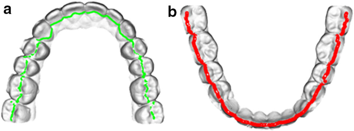
Ideally in clinical practice, the upper and lower teeth should be occluded as follows. In the incisal region, the upper and lower dental midlines should be perfectly aligned with each other (called midline alignment, Fig. 1a), while each lower incisal edge should make maximum contact to the palatal surface of the corresponding upper incisors. In the canine region, the upper canine should be visually aligned to the buccal side of the embrasure between the corresponding lower canine and first premolar (called Class I canine relationship, Fig. 1b). In the molar region, the mesiobuccal cusp of the upper first molars should be visually aligned to (the buccal side of) the developmental groove of the lower first molar (called Class I molar relationship, Fig. 1b).

Fig. 1.

Occlusion relationship: a midline alignment, b Class I relationship, c molar cusp–fossa relationship with maximum contact

Our automatic dental articulation approach is to digitally “replicate” the above steps that doctors do clinically. In addition, the molar relationship is determined by a true quantitative cusp–fossa relationship, rather than a qualitative visual alignment. That is, the mesiopalatal cusp of the upper first molar is seated in the central fossa of the corresponding lower first molar with maximum contact. Also, the distobuccal cusp of the lower first molar is seated in the central fossa of the corresponding upper first molar, also with maximum contact (Fig. 1c).

Our approach includes the following three major stages: (1) extract points of interest (POI) and detect additional teeth landmarks; (2) establish clinically desired Midline-Canine-Molar (M-C-M) relationship, and (3) establish final occlusion to achieve maximum contact between upper and lower dental models with collision and clinical (the desired M-C-M relationship) constraints. During the second and third stages, the upper dental model is mobile while the lower dental model remains static. The flowchart is shown in Fig. 2. Details of each stage are described below.

Fig. 2.

Flowchart of the algorithm

Extract points-of-interest and detect additional teeth landmarks

Each dental model is a triangulated mesh in STL format containing the teeth, braces, and gingiva parts. However, only the anatomical structures on the occlusal surface, including peaks (i.e., incisal edges and cusps) and valleys (i.e., fossae, embrasures and central grooves), are involved in the dental articulation. Therefore, we extract POI to represent these anatomical structures which are clinically important in guiding the digital articulation. While most teeth landmarks (with known anatomical definitions and names) are already digitized by surgeons during the surgical planning process (Table 1), it is necessary to detect the teeth landmarks that are not commonly used for surgical planning but important for articulation (Table 2). The POI extraction and the teeth landmark detection are automatically achieved in the following four steps.

Table 1.

Clinically digitized teeth landmarks

Description	Abbreviation
Upper
Midpoint of the right and left central incisal edges	U0
Canine cuspa	U3C
Mesiobuccal cusp of the 1st molara	U6MBC
Mesiobuccal cusp of the 2nd molara	U7MBC
Lower
Midpoint of the right and left central incisal edges	L0
Canine cuspa	L3C
Mesiobuccal cusp of the 1st molara	L6MBC
Mesiobuccal cusp of the 2nd molara	L7MBC

^aBilateral landmark

Table 2.

Automatically detected teeth landmarks

Description	Abbreviation
Upper
Mesiolingual cusp of the 1st molara	U6MLC
Central fossa of the 1st molara	U6CF
Lower
Embrasure between canine and the 1st premolara	L34Embr
Distobuccal cusp of the 1st molara	L6DBC
Central fossa of the 1st molara	L6CF

^aBilateral landmark

Extraction of occlusal surface

The patient’s dental models usually include braces, gums and base, which cause severe interference for the digital articulation. This step is to extract the occlusal surface by digitally removing the braces and gums with the guidance of the already digitized teeth landmarks. The digitized landmarks are shown in Fig. 3 and listed in Table 1.

Fig. 3.

Landmarks for digital occlusion (red: digitized; green: detected): a upper teeth landmarks, b lower teeth landmarks

For each dental model, seven already digitized teeth landmarks (Table 1) are first used to create a 200-point fitting curve Cur₁ (Fig. 4a) and a plane P₁ by principle component analysis (PCA). Then Cur₁ is projected onto P₁, denoted by Cur′₁. Each vertex υ (point) of the dental model is also projected to P₁, denoted by υ′. The distance h_υ between υ and υ′ is calculated for each vertex. After that, the distance r_υ between each projected vertex υ′ and the projected fitting curve Cur′₁ is calculated. The vertices of the occlusal surface are ultimately extracted using k-means clustering method. A threshold H is set empirically for h_υ. For each vertex u satisfying h_u < H, we define a parameter ϕ_u ≔ α · h_u + β · r_u, where coefficients α and β satisfy α + β = 1.We empirically choose the values as H = 15 mm, α = 0.2. The values of α and β control the importance of h_u and r_u in parameter ϕ_u. In the next step, k-means clustering algorithm is performed using parameter ϕ_u. Among the acquired clusters, we only keep the cluster for the occlusal surface (Fig. 4b). Finally, 200 cross-sectional planes are created, one for each point on Cur′₁. The intersection of the plane and occlusal surface and subsequently its envelope Env are calculated. Figure 4c shows one envelope as an example. The envelopes are used to further classify the peaks and valleys on the occlusal surface.

Fig. 4.

Occlusal surface extraction: a fitting curve, b extracted occlusal surface, c intersection plane and envelope

POI classification

Each envelope consists of three POIs: one valley in the middle and two peaks, one on each side (buccal and palatal/lingual). We first detect the points of the prominent peak on one side, then the second peak on the other side, and finally the points of the valley.

Detect the points of the first (the prominent) peak

A plane P₂ is created. It is parallel to P₁ with a distance in the direction away from the occlusal surface (Fig. 5a). We empirically use 15 mm as this distance to ensure that P₂ does not touch the occlusal surface. The vertices on each envelope are then classified by calculating the distance between each vertex to P₂. If the distance is greater than the both of its two neighbors, this vertex is classified as the local minimum point; if the distance is smaller than its neighbors, it is classified as the local maximum point. The local maximum point with the smallest distance to P₂ is the most prominent peak point on each envelope (red point in Fig. 5a).

Fig. 5.

POI classification: a detect most prominent peak point, b envelop simplification, c find a concave separation point, d detect second peak point

Detect the points of the second peak

The detection of the points of the second peak is more complex. Due to the teeth anatomy, the point with the second smallest distance is not the second peak’s point. We use the following strategy to detect the second peak’s points.

First, the envelopes of seven teeth landmarks are simplified using Douglas–Peucker algorithm (Fig. 5b). To begin, the first and last vertices of the envelope are marked as initial neighboring “keep” points. Next, each pair of two neighboring “keep” points are connected by a line segment. A distance is then calculated from each vertex on the envelope segment between the two neighboring “keep” points to the line segment. We mark the vertex that has the largest distance as “keep” if the distance is greater than an empirically defined threshold ε ≔ 0.01 mm. Once a set of new “keep” points is found, the algorithm iteratively forms new line segments and repeats the above steps.

After the simplification of the seven envelopes, each “keep” point is classified as either convex (red points in Fig. 5c) if it falls on the convex part of the envelope, or concave (green points in Fig. 5c) if it falls on the concave part. A distance between each concave point and P₂ is calculated. Only the concave point with the largest distance is selected, one for each corresponding envelope.

A new 200-point fitting curve Cur₂ is created based on the seven concave points. Each point p ∈ Cur₂ is first projected onto its corresponding cross-sectional plane as p′, which is then projected again to the envelope and becomes a separation point, that divides each envelope into two segments, S₁ and S₂.

Assume the first (the prominent) peak’s point falls onto one of the two envelope segments S₁. To detect the second peak’s point on segment S₂, a straight line is first constructed by connecting the first peak’s point and the separation point. All the local maximum points on S₂ that are above the straight line and in the direction away from the occlusal surface are selected. The distances between each of the selected local maximum points and the straight line are then calculated. The second peak’s point is the point with the largest distance (red point on the right in Fig. 5d).

Detect the points of the valley

To detect the (deepest) valley point on each envelope, a straight line is created by connecting the two peak points. All the local minimum points below the straight line (in the direction toward the occlusal surface) and located between the two peak points are selected. We calculate the distance from each of the selected points to the straight line. The valley point is the point with the largest distance (dark green point in Fig. 5d).

Finally, there are no valley points on the anterior teeth. Clinically, we use a hypothetical line that is extended from the valleys of the upper premolar and molars to the palatal surfaces of the anterior teeth to estimate where the lower incisal edges should occlude. In our approach, the hypothetical valley points of the anterior teeth are calculated as follows. The average distance from all premolar and molar valley points to P₂ is calculated. This is the same distance where the valley points are located on the palatal side of the upper incisors. (The valley points are shown in green in Fig. 6a.)

Fig. 6.

Extracted POI on a pair of teeth model: a upper model, b lower model

Detection of additional teeth landmarks

In addition to the clinically digitized teeth landmarks, five additional landmarks on each side are further needed for articulating the canine and molar relationships (green points in Fig. 3 and Table 2). They are automatically detected based on the anatomy of the teeth.

For the additional lower teeth landmarks: (1) landmark L34Embr is the embrasure between the canine and the first premolar. It is detected as the first local minimum buccal peak point, distal to the already digitized landmarks of the canine cusp (L3C). (2) Landmark L6DBC is the distobuccal cusp of the first molar. The developmental groove is initially detected as the first local minimum buccal peak point, distal to the already digitized mesiobuccal cusp of the first molar (L6MBC). Landmark L6DBC is then detected as the first local maximum buccal peak point, distal to the developmental groove. (3) Landmark L6CF is the central fossa of the lower first molar. It is the “lowest” valley point, within the boundaries of Landmarks L6MBC mesially and L6DBC distally.

For the additional upper teeth landmarks: (1) landmark U6MLC is the mesiopalatal cusp of the upper first molar. It is the local maximum palatal peak point, on the palatal side of the already digitized landmark of the mesiobuccal cusp of the upper first molar (U6MBC). (2) Landmark U6CF is the central fossa of the upper first molar. It is detected using the same method of detecting Landmark L6CF, by first detecting the developmental groove of the upper first molar, then the distobuccal cusp of the first molar (U6DBC). Landmark U6CF is then detected as the “lowest” valley point, within the boundaries of Landmarks U6MBC mesially and Landmark U6DBC distally.

Establish Clinically Desired Midline-Canine-Molar Relationship

In the second stage, the upper and lower dental models are aligned to the clinically desired M-C-M relationship. It is achieved in the following two steps: (1) a local coordinate system is established for each of the key landmarks on the lower dental model. These key landmarks are used for achieving M-C-M alignment. (2) The sum of distances is minimized between the upper and lower key landmarks.

Local coordinate system

During the dental alignment, the lower teeth model always remains static, while the upper dental model is translationally and rotationally transformed and articulated to the lower model. A local coordinate systems is built to establish a clinically desired M-C-M relationship on each of the 7 key landmarks of the lower teeth (Table 3).

Table 3.

Key landmarks used in M-C-M alignment

	Landmarks
Upper	U0	U3Ca	U6MLCa	U6CFa
Paired lower	L0	L34Embra	L6CFa	L6DBCa

^aBilateral landmark

To build a local coordinate system, the same occlusal plane P₁ for the lower teeth model is used. The normal vector of P₁, in the direction from the root to the crown of the teeth, is the z-axis of the local coordinates for all the landmarks. The lower landmarks list in Table 3 are then projected onto P₁, and a fitting curve Cur₃ is formed using these projected landmarks. The tangent line of Cur₃ at each projected landmark, along the direction from the (patient’s) right to the left side of the dental model, is the x-axis of each corresponding landmark. Last, the y-axis is calculated as the cross product of the z- and x-axes (Fig. 7, only one side of the landmarks are shown for bilateral landmarks).

Fig. 7.

Local coordinate system for lower teeth landmarks

Distance minimization

We jointly consider the three clinical requirements described in Method section. Clinically, the midline alignment and the canine relationship are more important than the molar relationship because it is difficult for orthodontists to correct the midline deviation and the canine relationship after the surgery, while it is much easier to close the space between upper and lower molars. For this reason, in our M-C-M alignment, we assign different weights to the dental midline alignment, the canine relationship and the molar relationship.

We use l_u to represent an upper tooth landmark and l_l to represent its corresponding lower tooth landmark. The local x-axis at each lower landmark is represented by x_l, and the transformation matrix for upper model is M. Thus each new upper landmark position becomes M · l_u.

For the midline alignment, we consider the deviation between U0 and L0 along the local x-axis. Let d_mi = M · l_U0 − l_L0 be a vector pointing from L0 to U0, and $d_{\text{mi}}^x=d_{\text{mi}}\cdot x_{L0}$ be the distance of d_mi along the local x-axis.

Similarly, for the canine relationship, we consider the off-set between the corresponding U3C and L34Embr on both right and left sides, also along their local x-axes. For each side, let d_C = M · l_U3C − l_L34Embr be the vectors pointing from L34Embr to U3C, and $d_C^x=d_C\cdot x_{\text{L}34\text{Embr}}$ be the distances of d_C along the local x-axis.

For the molar relationship, we consider the Euclidean distance between each paired upper and lower molar landmarks, i.e., the distances of U6MLC-L6CF and U6CF-L6DBC, respectively, on the right and the left sides. Let d_M1= M · l_U6MLC − l_L6CF and d_M2 = M · l_U6CF − l_L6DBC be the vectors pointing from the lower teeth landmarks to the corresponding upper teeth landmarks.

Three different weights, w₁, w₂ and w₃, are assigned to the distances of midline $d_{\text{mi}}^x$, canine $d_C^x$ and molar d_M1 and d_M2, respectively. They represent the importance ratio of the corresponding teeth taken into the M-C-M alignment. They are set to be 1 by default, indicating that midline, canine and molar are equally considered in the alignment. These weights can either be used by their default values or changed with user’s preference in our user interface. The summation of the above distances is $w_1\cdot d_{\text{mi}}^x+w_2\cdot d_C^x+w_3\cdot \left(d_{M1}+d_{M2}\right)$.

There are two clinical rules during the dental articulation: (1) the buccal cusps and incisal edges of the upper dental model are located at the buccal side of the lower teeth, and (2) the upper dental model is located superiorly to the lower dental model. The local y-axis and z-axis of each lower landmark are represented by y_l and z_l. The following constraints are used to guarantee the correct position of the dental models. For the midline and the canines, the constraints are d_mi · y_L0 < 0 and d_C · y_L34Embr < 0 (rule #1). For the molars, the constraints are d_M1 · z_L6CF > 0 and d_M2 · z_L6DBC > 0 (rule #2).

In order to avoid collision in M-C-M relationship, we modify (relax) the constraints for the molars as (M · l_U6MBC − l_L6MBC) · z_L6CF > 0. In addition, we also modify the constraints as d_C · z_L34Embr > 0 for the canines. This is to ensure U6MBC is above L6MBC, and U3C is above L34Embr.

Finally, the optimization function can be written as:

$$\text{Min}\left\{w_1\cdot d_{\text{mi}}^x+w_2\cdot d_C^x+w_3\cdot \left(d_{M1}+d_{M2}\right)\right\}$$

$$\text{s.t.\hspace{0.17em}}{d}_{\text{mi}}\cdot y_{L0}<0,$$

$$d_C\cdot y_{\text{L}34\text{Embr}}<0,$$

$$d_C\cdot z_{\text{L}34\text{Embr}}>0,$$

$$\left(M\cdot l_{\text{U}6\text{MBC}}-l_{\text{L}6\text{MBC}}\right)z_{\text{L}6\text{CF}}>0$$ (1)

Points-of-interest-based fine alignment

In this stage, the upper and lower dental models are finally articulated to the clinically desired final occlusion by iteratively minimizing the distance between the upper and lower POI. This is also to achieve a best possible maximum contact between the upper and the lower teeth. During articulation, we first match each upper teeth POI with a lower teeth POI. Then we calculate the collision constraint and M-C-M constraint based on current upper teeth location. Finally, we fine align the teeth model by minimizing the distance between matched POI under these two constraints. The details are described below.

Point match of upper and lower POI

The upper and lower teeth should follow a cusp–fossa inter-cuspation relationship. That is, the central groove (i.e., the valley points) of the upper teeth should be seated on top of the buccal cusps (i.e., the buccal peak points) of the lower teeth for the premolars and molars. The palatal side of the upper incisors and canines (i.e., the hypothetical valley points at the palatal side of the upper anterior teeth) should also have a maximum contact with the lower incisors and canines edges (i.e., the peak points of lower anterior teeth). Similar to the M-C-M stage that each upper teeth landmark is paired with a lower teeth landmark, each vertex of the upper POI (green points in Fig. 6a) is paired with a lower POI (red points in Fig. 6b). Let {u_i} be the upper POI and {l_j} be the lower POI. The pairing process is to find a l_ji for u_i, such that $l_{j_i}=\text{arg\hspace{0.17em}}{\text{min}}_{l\in \left\{l_j\right\}}{u}_i-l$.

Collision constraint

Collision constraint is applied to guarantee that upper and lower models do not penetrate into each other. Theoretically, the penetration depth of upper and lower models should be 0 when there is no collision. However, due to the reconstruction error of triangulated.STL models, we empirically allow 0.1 mm of penetration depth. Clinically, this small allowance does not result in collision between the upper and lower dental models.

Let {U_i} be the vertices on the extracted upper occlusal surface and {L_j} be the vertices on the extracted lower occlusal surface. To detect collision, each upper occlusal surface vertex U_i is paired with the closest vertex L_ji on the extracted lower one using the same method described in the point match section above. The penetration depth is calculated as the distance that the upper vertex penetrated into the lower model, in the direction of the normal vector n_j of the paired lower vertex. The penetration is formulated as

$$\left(R\cdot U_i+t-L_{ji}\right)\cdot n_{ji}+\epsilon >0$$

where R is rotational matrix and t is translational matrix, and ε is the penetration depth we set empirically.

Clinical M-C-M constraint

In addition to the collision constraint, M-C-M relationship also needs to be maintained during the fine alignment. It is achieved by constraining the movement of the landmark U0 by setting user-adjustable thresholds for its moving distances along three local coordinate axis separately. By default, the movement threshold along x-axis guarantees that the alignment of the upper and lower midlines is within clinically acceptable deviation (0.5 mm, i.e., $d_{\text{mi}}^x<0.5$). In addition, the movement threshold along y-axis is set to 1 mm toward the labial side to constrain the overjet (normal value: 1.5–4.0 mm), while the movement toward the lingual side is automatically constrained by collision. Finally, the movement threshold along z-axis is set to be 0.2 mm deviating from the lower teeth to constrain the overbite (normal value 1.5–4.0 mm), while the movement toward the lower teeth direction is also automatically constrained by collision. Within such a small amount of the movement, we believe the midline alignment, and canine and molar relationships will not be significantly changed.

Distance minimization

The goal of this step is to find the transformation matrix for the upper dental model with the minimized overall distance between paired POI {u_i} and $\left\{l_{j_i}\right\}$ with the collision and the M-C-M constraints. In each iteration, the model is rotated around a pivot center and then translated to minimize the overall distances between current paired {u_i} and $\left\{l_{j_i}\right\}$. The pivot center is found based on the distances between upper and lower teeth vertices. We calculate the pivot center as

$$\tilde{o}\leftarrow \frac{{\sum }_i{w}_i{u}_i}{{\sum }_i{w}_i}.$$ (2)

where $w_i\propto e^{-\Vert u_i-l_{j_i}\Vert }$ is a weight assigned to vertex u_i. Then the distance is minimized by solving

$$\text{Min}\sum _{i=1}^{n}R\left(u_i-\tilde{o}\right)+\tilde{o}+t-l_{ji}^2$$ (3)

where R is rotational matrix and t is translational matrix. After each iteration is completed, the upper vertices will be re-paired with lower vertices using point match described in Sect. 3.3, and the iteration will continue until (3) converges.

Experiment and results

Materials and methods

Patient dental models between February 2017 and August 2018 were randomly selected from our large patient archive to evaluate the accuracy and efficiency of our method qualitatively and quantitatively (IRB #Pro00003644). The inclusion criteria were: (1) patients had undergone double-jaw orthognathic surgery, (2) maxillary surgery was a one-piece nonsegmental Le Fort I osteotomy, (3) the occlusion was stable without rocking between the upper and lower dental models. Partially edentulous models were not excluded. A convenient sample size of 18 sets of dental models were finally selected and used for the evaluation. Of these 18 patients, three were edentulous cases who had upper and lower first premolars extracted on both sides.

The paired upper and lower digital dental models were generated by scanning the upper and lower dental stone models separately using a cone-beam computed tomography (CBCT) scanner (iCAT, Hatfield, Pennsylvania, United States). Once the landmarks were digitized (following the clinical routine of surgical planning), our approach was applied to automatically articulate the upper and lower models to the final occlusion. We used the default values for the weight w₁, w₂ and w₃, i.e., w₁ = w₂ = w₃ = 1. The algorithm-articulated occlusions served as the experimental group.

To generate the ground truth, the upper and lower stone models were hand-articulated by two experienced orthodontists (F.G and R.E.). The hand-articulated stone models were scanned together as a whole using the same CBCT scanner, forming a final occlusal template. The separately scanned digital dental models were registered to the corresponding final occlusal template, resulting in the digital representation of the hand-articulated occlusions. This process is also the clinical routine in CASS-based surgical planning. [1] They served as the control group.

During the qualitative evaluation, the same two orthodontists, who were blinded from the articulation methods, compared the results of the experimental and control groups. Both were displayed in pair, side by side, on a large screen monitor. The orthodontists were able to freely rotate, show/hide and zoom in/out of the articulated digital dental models. They were also able to verify results in the computer using the corresponding stone models. A 3-scale visual analog scale (VAS, (1) the first set was better than the second set; (2) they were equal; and (3) the first set was worse) was used.

During the quantitative evaluation, we measured the distances of the midline landmarks (U0-L0) and the canine landmarks (U3C-L34Embr) along their local x-axes, and averaged Euclidean distances of molar landmarks (U6MLC-L6CF). In order to avoid possible human error caused by manual landmark digitization, the landmarks were only digitized on one model, either in experimental or control group. This model was then automatically registered to the other using surface-best-fit method, bringing the landmarks along with it [8, 9]. Finally, repeated measures analysis of variance (ANOVA) was performed to compare the measurements between experimental and control groups. Response variable was the distance between the paired landmarks. Within-factors were 2 methods (algorithm articulation and hand articulation) and 5 locations (midline, right and left canines, and right and left first molars). The assumption for the repeated measures ANOVA was tested and could not be rejected. If there was a statistically significant difference between the 2 methods, the within contrast would be further computed and the results would be reported separately. If there was no statistically significant difference, Bland and Altman method for accessing measurement agreement [10] would be used to report the difference between the algorithm-articulated and the hand-articulated occlusions.

Results

Our 3-step approach was successfully used to establish the final occlusion on all 18 pairs of the models. The maximal time spent on the entire process of running our 3-stage approach for each articulation was within 3 min.

The results of the qualitative evaluation showed that all 18 algorithm-articulated models were as good as the hand-articulated ground truth models, including the edentulous cases. A randomly selected case is shown in Fig. 8.

Fig. 8.

Occlusion result (left: algorithm-articulated, right: hand-articulated)

The results of repeated measures ANOVA showed there was no statistically significant difference in the resulted occlusions between the two methods (F[1, 16] = 0.02, P = 0.88). Therefore, within contrast was not further computed. The mean distances are compared in Table 4. The results of Bland and Altman’s measurement agreement are shown in Table 5. The average of the measurement differences between the two methods are less than 0.22 mm, and the lower and upper limits of the measurement differences are within the range of [− 1.31, 1.25].

Table 4.

Mean distance comparison (mm)

Measurement	Algorithm	Hand
Midline	−0.16	0.06
Canine (R)	1.44	1.23
Canine (L)	−0.73	−0.83
Molar (R)	2.10	2.03
Molar (L)	2.36	2.48

Table 5.

Bland and Altman’s measurement (mm)

Measurement	Mean	STD	Lower limit	Upper limit
U0	−0.22	0.37	−0.94	0.51
CR	0.21	0.47	−0.72	1.14
CL	0.1	0.57	−1.02	1.22
MR	0.07	0.61	−1.12	1.25
ML	−0.12	0.61	−1.31	1.07

Discussion and conclusion

Our new method is capable of automatically articulating the digital dental models to the clinically desired final occlusion, including several partial edentulous cases. The entire process of our method is completed within 3 min.

The prior knowledge is the landmarks which were clinically digitized for surgical planning. Although our study and some previous studies are able to detect landmarks by capturing certain features of the teeth, Lu et al. [11] proposed a machine learning-based method that can identify teeth as incisor, canine, premolar and molar. However, they are not able to detect the correct name for each landmark, especially for the teeth with similar teeth anatomy (e.g., first premolar and second premolar) and for those edentulous models (either with or without space between teeth).

There are studies using curvature-based methods for dental feature extraction and segmentation. Kumar et al. [12] developed mesh-based method to automatically detect cusps, ridges, grooves features. Wu et al. [4] used mean principal curvature to separate teeth for scanned dental meshes. Kumar et al. [13] used minimum principal curvature for teeth segmentation. Wu et al. [14] proposed a method which used mean curvature and morphologic skeleton operation to identify teeth boundaries. Mouritsen [15] proposed a method to segment teeth with an automatically adjusted curvature threshold and morphologic skeleton. However, the curvature threshold is difficult to estimate. Wang and Li [16] proposed a method based on segmentation field. However, user interaction is needed to assign boundary constraints. Surface curvature is sensitive to the anatomical structure of the teeth. However, in real life, the teeth anatomy may be different from patient to patient due to the chewing habit, teeth grinding, or developmental variations. There are also studies that developed an interactive tooth partition method based on harmonic field and prior knowledge of teeth landmarks [17, 18]. However, braces will also change the shape and features of the teeth. We also developed a projected height-based method [5] to extract the dental feature points, in which the teeth boundary on the projection plane played an important role. However, it is also problematic when the model has braces and the structures other than the teeth, e.g., gums and the base of the dental models. These unnecessary structures significantly alter the projected teeth shape; thus, it does not work well on un-preprocessed dental models. The above methods are extremely sensitive to the orthodontic braces as they have similar geometric features as the edge and cusps. Therefore, they cannot be used on the dental models with the orthodontic braces, which nearly every patient undergoing jaw surgery would have. There are studies that integrate human interaction into the teeth segmentation. [19, 20] (This paper is based on the work [7].) They have relative accurate results but need extensive human labor work.

In an effort to digitally articulate dental models, Wu et al. [4] proposed a physically based haptic simulation method to manually articulate the digital model. Nadjmi et al. [3] proposed a method using a “spring connection” to articulate the models to a stable position. It required the users to first move the upper teeth model to a good initial position and then indicate at least three pairs of points on the models for the “spring.” The “spring connection” would generate force to bring upper and lower teeth together. It was not an automatic process. The articulation was highly dependent on the “lucky” initial position and the point selection. Thus, the user needed to iteratively find proper initial position in order to achieve an articulation.

In summary, our proposed method does not require model pre-processing and the whole articulation process is fully automatic. The final occlusion result does not rely on the initial position of the teeth model, and they are evaluated to be equally good as the current gold standard. The clinical contribution of this method is significant. It allows doctors to eliminate the use of stone dental models and obtain a clinically desired final occlusion in the computer that is equally as good as the hand-articulated result. Finally, we are currently working on new digital articulation functions for multi-piece maxillary surgery, as well as for surgery-first orthognathic surgery.

References

- 1.Xia JJ, Gateno J, Teichgraeber JF, Yuan P, Chen KC, Li J, Zhang X, Tang Z, Alfi DM (2015) Algorithm for planning a double-jaw orthognathic surgery using a computer-aided surgical simulation (CASS) protocol. Part 1: planning sequence. Int J Oral Maxillofac Surg 44(12):1431–1440. 10.1016/j.ijom.2015.06.006 [DOI] [PMC free article] [PubMed] [Google Scholar]
- 2.Chabanas M, Marecaux C, Payan Y, Boutault F (2002) Models for planning and simulation in computer assisted orthognatic surgery. In: Paper presented at the proceedings of the 5th international conference on medical image computing and computer-assisted intervention-Part II [Google Scholar]
- 3.Nadjmi N, Mollemans W, Daelemans A, Van Hemelen G, Schutyser F, Berge S (2010) Virtual occlusion in planning orthognathic surgical procedures. Int J Oral Maxillofac Surg 39(5):457–462. 10.1016/j.ijom.2010.02.002 [DOI] [PubMed] [Google Scholar]
- 4.Wu W, Chen H, Cen Y, Hong Y, Khambay B, Heng PA (2017) Haptic simulation framework for determining virtual dental occlusion. Int J Comput Assist Radiol Surg 12(4):595–606. 10.1007/s11548-016-1475-3 [DOI] [PubMed] [Google Scholar]
- 5.Chang YB, Xia JJ, Gateno J, Xiong Z, Zhou X, Wong ST (2010) An automatic and robust algorithm of reestablishment of digital dental occlusion. IEEE Trans Med Imaging 29(9):1652–1663. 10.1109/TMI.2010.2049526 [DOI] [PMC free article] [PubMed] [Google Scholar]
- 6.Xia JJ, Chang YB, Gateno J, Xiong Z, Zho X (2010) Automated digital dental articulation. Med Image Comput Comput Assist Interv 13(Pt 3):278–286. 10.1007/978-3-642-15711-0_35 [DOI] [PMC free article] [PubMed] [Google Scholar]
- 7.Deng H, Yuan P, Wong S, Gateno J, Garrett FA, Ellis RK, English JD, Jacob HB, Kim D, Xia JJ (2019) An automatic approach to reestablish final dental occlusion for 1-piece maxillary orthognathic surgery 2019 medical image computing and computer assisted intervention–MICCAI 2019. Springer, Cham, pp 345–353 [DOI] [PMC free article] [PubMed] [Google Scholar]
- 8.Xia JJ, Gateno J, Teichgraeber JF, Christensen AM, Lasky RE, Lemoine JJ, Liebschner MA (2007) Accuracy of the computer-aided surgical simulation (CASS) system in the treatment of patients with complex craniomaxillofacial deformity: a pilot study. J Oral Maxillofac Surg 65(2):248–254. 10.1016/j.joms.2006.10.005 [DOI] [PubMed] [Google Scholar]
- 9.Hsu SS, Gateno J, Bell RB, Hirsch DL, Markiewicz MR, Teichgraeber JF, Zhou X, Xia JJ (2013) Accuracy of a computer-aided surgical simulation protocol for orthognathic surgery: a prospective multicenter study. J Oral Maxillofac Surg 71(1):128–142. 10.1016/j.joms.2012.03.027 [DOI] [PMC free article] [PubMed] [Google Scholar]
- 10.Bland JM, Altman DG (1986) Statistical methods for assessing agreement between two methods of clinical measurement. Lancet 1(8476):307–310 [PubMed] [Google Scholar]
- 11.Lu S, Yang J, Wang W, Li Z, Lu Z (2018) Teeth classification based on extreme learning machine. In: Paper presented at the 2018 second world conference on smart trends in systems, security and sustainability (WorldS4), 30–31 Oct 2018 [Google Scholar]
- 12.Kumar Y, Janardan R, Larson B (2012) Automatic feature identification in dental meshes. Comput Aided Des Appl 9(6):747–769. 10.3722/cadaps.2012.747-769 [DOI] [Google Scholar]
- 13.Kumar Y, Janardan R, Larson B, Moon J (2011) Improved segmentation of teeth in dental models. Comput Aided Des Appl 8:211–224. 10.3722/cadaps.2011.211-224 [DOI] [Google Scholar]
- 14.Wu K, Chen L, Li J, Zhou Y (2014) Tooth segmentation on dental meshes using morphologic skeleton. Comput Gr 38:199–211. 10.1016/j.cag.2013.10.028 [DOI] [Google Scholar]
- 15.Mouritsen DA (2013) Automatic segmentation of teeth in digital dental models. University of Alabama, Birmingham [Google Scholar]
- 16.Hao W, Zhongyi L (2016) Tooth separation from dental model using segmentation field. Conf Proc IEEE Eng Med Biol Soc 2016:5616–5619. 10.1109/embc.2016.7592000 [DOI] [PubMed] [Google Scholar]
- 17.Liao SH, Liu SJ, Zou BJ, Ding X, Liang Y, Huang JH (2015) Automatic tooth segmentation of dental mesh based on harmonic fields. Biomed Res Int 2015:187173 10.1155/2015/187173 [DOI] [PMC free article] [PubMed] [Google Scholar]
- 18.Zou BJ, Liu SJ, Liao SH, Ding X, Liang Y (2015) Interactive tooth partition of dental mesh base on tooth-target harmonic field. Comput Biol Med 56:132–144. 10.1016/j.compbiomed.2014.10.013 [DOI] [PubMed] [Google Scholar]
- 19.Sinthanayothin C, Tharanont W (2008) Orthodontics treatment simulation by teeth segmentation and setup. In: Paper presented at the 2008 5th international conference on electrical engineering/electronics, computer, telecommunications and information technology, 14–17 May 2008 [Google Scholar]
- 20.Ma Y, Li Z (2010) Computer aided orthodontics treatment by virtual segmentation and adjustment. In: Paper presented at the 2010 international conference on image analysis and signal processing, 9–11 Apr 2010 [Google Scholar]