

Abstract
Objective:
Medial temporal lobe epilepsy (TLE) is the most common form of medication-resistant focal epilepsy in adults. Despite removal of medial temporal structures, over a third of patients continue to have disabling seizures post-operatively. Seizure refractoriness implies that extra-medial regions are capable of influencing the brain network and generating seizures. We tested whether abnormalities of structural network integration could be associated with surgical outcomes.
Methods:
Presurgical magnetic resonance images from 121 patients with drug-resistant TLE across three independent epilepsy centers were used to train feed-forward neural network models based on tissue volume or graph-theory measures from whole-brain diffusion tensor imaging structural connectomes. An independent dataset of 47 patients with TLE from three other epilepsy centers was used to assess the predictive values of each model and regional anatomical contributions towards surgical treatment results.
Results:
The receiver-operating characteristic (ROC) area under the curve (AUC) based on regional betweenness centrality was 0.88, significantly higher than a random model or models based on gray matter volumes, degree, strength, and clustering coefficient. Nodes most strongly contributing to the predictive models involved the bilateral parahippocampal gyri, as well as the superior temporal gyri.
Interpretation:
Network integration in the medial and lateral temporal regions was related to surgical outcomes. Patients with abnormally integrated structural network nodes were less likely to achieve seizure freedom. These findings are in line with previous observations related to network abnormalities in TLE and expand on the notion of underlying aberrant plasticity. Our findings provide additional information on the mechanisms of surgical refractoriness.
Introduction
Focal epilepsies are characterized by recurrent seizures with onset in localized brain areas. The ictal-onset zone is defined as the area that generates aberrant epileptiform activity and can thus initiate clinical seizures1. In medial temporal lobe epilepsy (TLE), the ictal-onset zone is commonly assumed to be in the amygdala-hippocampo-parahippocampal complex2. Removal/disruption of the this region should therefore eliminate the emergence of anomalous electrical activity and control seizures. Indeed, resection or thermoablation of this medial temporal lobe complex can cure seizures in 40–65% of patients with drug-resistant TLE3–6. The remainder of patients with TLE remain with seizures after surgery and the reasons for suboptimal results in these patients remain undefined. Even with the most modern pre-surgical clinical assessment, patients who do not achieve post-surgical seizure control are virtually indistinguishable from those who fully benefit from surgery.
Imaging studies have demonstrated brain network reorganization extending beyond the ipsilateral medial temporal structures in TLE, predominantly affecting gray and white matter structures within, but not limited to, the limbic network7–9, with progressive widespread atrophy seen with longer disease duration10. In particular, extra-medial temporal damage in TLE may be a cause or a consequence of seizure, or both. Among other reasons, it may result from the excitotoxic effect of seizure spread or deafferentation due to hippocampal cell loss2, 11. At least two important neuroimaging findings corroborate the epileptogenic potential of extra-hippocampal tissue: lesion-symptom mapping studies demonstrating that resection/ablation extending beyond the hippocampus is more likely to yield seizure freedom12, 13; and multimodal data confirming that structural changes are associated with network reconfigurations through which certain brain regions acquire functional influence over neighboring structures14, thus becoming highly integrated nodes that contribute to seizure onset and propagation1, 15. The pathological role of these atypical network hubs in epilepsy is now better appreciated by assessing the topology of brain networks, i.e., the brain connectome. There is a robust overlap between abnormally strong connections and increased ‘centrality’ of ictal-onset zones to sites of non-contiguous spread in the structural connectome along with increased amplitude of cortico-cortical evoked potentials to those same distant sites (effective connectome)16. Seizure freedom is seen in association with statistical models that virtually resect hyper-connected17 and hyper-synchronized18 network hubs. Moreover, post-operatively, node-based measures of centrality rather than global network measures are associated with post-operative outcomes19. Nonetheless, the relationship between epilepsy-related network reconfiguration, network epileptogenic potential, and clinical phenotypes has not been fully assessed in TLE. In particular, it remains to be defined if network configurations are reproducibly associated with surgical outcome phenotypes across multiple sites.
Here, we hypothesize that personalized profiles of regional structural network influence can be used to predict TLE surgical outcomes. In particular, based on the cumulative evidence from grey and white matter changes in TLE summarized above, we propose that the hubness of different regions within the ipsilateral and contralateral medial and lateral temporal cortices will be associated with surgical outcomes. We employ machine learning to test this hypothesis on a large multicentric cohort of patients to evaluate the value of neuroimaging-based phenotypes in predicting surgical outcomes.
Methods
Patient inclusion and classification
A total of 168 participants were retrospectively identified from consecutive research cohorts of patients with an established diagnosis of drug-resistant unilateral TLE based on International League Against Epilepsy20 criteria from six academic epilepsy centers and grouped into a training set and an independent testing set, as follows:
The training cohort (n = 121) included patients from 1) the Medical University of South Carolina (MUSC, n = 45), SC, USA; 2) Emory University (EMORY, n = 32), GA, USA; and 3) University Hospital Bonn (BONN, n = 42), Germany.
The testing cohort (n = 47) included patients from 1) the University of California San Diego (UCSD, n = 17); 2) the University of California San Francisco (UCSF, n = 21); and 3) the University of Pennsylvania (PENN, n = 9).
Each patient diagnosis was the result of standard workup at each site, including video EEG monitoring, structural imaging, PET/SPECT, and Phase II monitoring as needed in each case. In all cases, unilateral temporal lobe onset was confirmed by a multi-disciplinary group in charge of reviewing refractory epilepsy cases at each site. IRB approval was independently obtained at each institution for respective ongoing studies of neuroimaging in epilepsy. Patients were included in the present analysis if they had undergone pre-surgical diffusion magnetic resonance imaging and if seizure outcome data were available at 12 months after the date of surgery, which could be either laser interstitial thermal therapy or resection. Based on in-person interviews and assessment of patients during standard clinic follow up, the surgical outcome was defined based on the Engel Surgical Outcome scale21 as either seizure-free (SF; Engel Class I) or not seizure-free (NSF; Engel Class II through IV).
Image acquisition
All images were acquired preoperatively on a 3T MRI scanner. Scanner type and acquisition parameters varied across institutions, as follows:
MUSC: Siemmens Skyra 3T scanner (12-channel head coil); T1-weighted image: isotropic voxel size of 1mm (TR = 2050–2250 ms, TE = 2.5–18 ms, FOV = 256– 320 mm, flip angle 10°); diffusion-weighted data: 30 directions (TR = 10,600–12,000 ms, TE = 99–100 ms, FOV = 74–112 mm, parallel imaging factor of 2, slice thickness = 2 mm, 60 axial slices, isotropic voxel size of 3 mm, GRAPPA)
EMORY: Siemens Skyra 3T scanner (12-channel head coil); T1-weighted image: isotropic voxel size of 0.8mm (TR = 2300ms, TE = 2.75ms, TI = 1100ms, flip angle 8°); diffusion-weighted data: 60 directions (TR = 3430ms, TE = 90ms, FOV = 224mm, 81 slices, isotropic voxel size of 1.75 mm GRAPPA)
BONN: Siemens Magnetom Trio 3T scanner (8-channel head coil); T1-weighted image: isotropic voxel size of 1mm (TR = 650ms, TE = 3.97ms, TI = 650ms, flip angle 10°); diffusion-weighted data: 60 directions (TR = 1200ms, TE = 100 ms, 72 axial slices, voxel size 1.726 × 1.726 × 1.7 mm, no cardiac gating, GRAPPA).
UCSD/UCSF: General Electric Discovery MR750 3T scanner (8-channel phased-array head coil); T1- weighted image: isotropic voxel size of 1mm (TR = 8.08 ms, TE = 3.16 ms, TI = 600 ms, flip angle 8°); diffusion-weighted data: 30 directions
PENN: Siemens Prisma 3T (32-channel head coil); T1-weighted image: isotropic voxel size of 0.8 mm (TR = 2400ms, TE = 2.24ms, TI = 1060ms); diffusion-weighted data: 117 directions (TR = 4300ms, TE = 75ms, 76 axial slices).
Gray matter volumes
Regional average gray matter volumes were obtained by processing the T1-weighted images using an approach similar to pre-processing for voxel-based morphometry22. Using the software package Statistical Parametric Mapping (SPM), the T1-weighted images were initially normalized to standard space and segmented into gray matter probability maps using an iteratively optimized normalization – segmentation approach23, which has been previously used for patients with epilepsy24. Using Matlab scripts developed in-house, the resulting modulated tissue maps were parcellated into regions of interest (ROI) following the Atlas of Intrinsic Connectivity of Homotopic Areas (AICHA)25 and the average voxel-wise modulated tissue probability was extracted from each ROI. The output from this process was an individual measure of the volume of each ROI per each patient.
Diffusion tensor imaging structural connectome
The individual connectome was computed from each patient’s presurgical diffusion sequences based on the following steps: 1) a probabilistic gray matter map was derived from T1-weighted sequences and segmented into 384 regions of interest (ROIs) based on the Atlas of Intrinsic Connectivity of Homotopic Areas (AICHA)25 with 192 ROIs for each hemisphere; 2) an individual probabilistic white matter map was derived from T1-weighted sequences to guide fiber tracking; 3) the white matter map and the 384 grey matter ROIs were registered into the individual diffusor tensor imaging (DTI) space; 4) probabilistic DTI fiber tracking between all possible pairs of ROIs was performed using FSL’s Bedpostx and Probtrackx26, which yielded the number of probabilistic streamlines arriving in one ROI, when another ROI was seeded, using the white matter as the waypoint. Fiber tracking was performed using FSL FDT’s probabilistic tractography method (RRID: SCR_002823)27. Specifically, seeding one ROI at a time (i), the number of probable streamlines arriving at another ROI (j) was computed, averaging the connections from ROIi to ROIj and vice versa. The number of streamlines was then corrected by the distance between ROIs and by the sum of the volume of the ROIs to account for variability in anatomical separation and size of different ROIs, respectively. To account for independent left and right pathology, individual connectomes were rearranged so that ROIs represented ipsilateral vs. contralateral (to the side of surgery) areas rather than a left vs. right dichotomy. For example, for a patient with right-sided TLE, ROIs on the right hemisphere became ipsilateral, whereas ROIs in the left hemisphere were considered contralateral. This process yielded an individual matrix M per patient of size 384×384, where each cell Mij represented the corrected weight of the connection between ROI i and ROI j.
Data harmonization
To control for the potential effect of scanner type, T1- and DTI-derived individual values (i.e., ROI volumes and connectivity strengths) were homogenized by applying ComBat, a well-established approach originally designed to adjust batch effects in microarray expression data28, but more recently validated specifically for diffusion tensor imaging29 including particularly in multi-site cohorts of patients with epilepsy30. More specifically, ComBat removes unwanted variation introduced by site while preserving biological variability using a Bayesian framework that estimates an empirical statistical distribution for each parameter by assuming that all voxels share the same common distribution.
Graph theory measures
Graph theory measures were derived from each participant’s individual post-ComBat connectome to characterize nodal (e.g. ROI-based) topological properties of the network. We computed four topological measures (see below) for all 384 ROIs using the Brain Connectivity Toolbox31 for MatLab. The measures chosen for this study describe different properties of each node (i.e., region) and reflect the organization of the brain network at each of its vertices. We computed the following topological measures that have been thoroughly investigated in patients with epilepsy32, 33:
degree (Deg), which is the total number of edges connected to a node in the network; in other words, a measure of how many connections arrive to/depart from each ROI (higher degree = more connections to/from a given ROI);
strength (Str), the average weight of all edges connected to a node; in other words, a measure of how prominent (independently of how numerous) the connections of each ROI are (higher strength = more prominent connections to/from a given ROI);
cluster coefficient (CC), the proportion of a node’s neighbors (i.e., contiguous nodes) that are also neighbors of each other; in other words, a measure of the fraction of triangles around each node, which reflects the degree to which ROIs in the network tend to cluster together (higher clustering coefficient = a ROI’s neighbors are more connected to each other);
betweenness centrality (BC), the proportion of shortest paths in the network that pass through a particular node; in other words, the degree to which other regions rely on a particular node for efficient (i.e., shortest amount of steps needed) flow of information. A higher value of BC indicates a more highly integrated region within the network.
Based on the mathematical definition of these four measures, BC is the measure that most strongly reflects network integration at the nodal level, followed by CC, Str, and Deg in decreasing fashion. An example is shown in the bottom panel of Figure 1. A highly connected node (labeled “High Degree” on the sample diagram) is not as influential on the network as a node with high BC since the information would still be able to flow with relative efficiency if the former were to be lost. On the contrary, the node with high BC is essential for information flow between the nodes on the left and right sides of the sample network.
Figure 1.

Overview of the methods and framework of the study. The top left pannel shows the segmentation into grey (GM) and white matter (WM) maps based on an individual patient’s T1-weighted magnetic resonance imaging. The GM is then parcellated into ROIs based on the AICHA atlas (top right panel). This is used to generate the GM volumes used for model prediction. Probabilistic tractography is computed to generate white matter pathways (for visualization purposes, the deterministic white matter tractography results from one subject is shown above). White matter connections across all GM ROIs are computed and input into a 2D adjacency matrix (the individual connectome), where each row i and column j represent an ROI, and the value of ij is the strength of structural connectivity between those two GM structures. The bottom panel demonstrates a sample hypothetical graph with twelve nodes. Note the key difference between a node with high degree (five connections, but if this node disappeared, information would still flow efficiently throughout the rest of the network) versus a node with high betweenness centrality (BC; only four connections, but if this node disappeared, information flow would be limited). The left lateral brain views on the bottom panel demonstrate the different patterns of connections in two representative patients with high (left brain diagram) vs. low (right brain diagram) betweenness centrality values of the left hippocampus. For each patient, the structural connections to the hippocampi are color coded so that connections to the left hippocampus are shown in bright blue, then the connection from the node connected to the hippocampus to its other connected structures are shown in fainter blue and so forth. Visually, it is possible to appreciate a higher density of connected subnetworks in the hippocampus with higher BC.
Even though the structural connectome was calculated based on the entire brain (384 ROIs), to avoid model overfitting, we selected 56 ROIs (AICHA regions 161–188 and 317–344, 383–384) to be used in the machine learning models. These ROIs were chosen to represent archi-, paleo- and neocortical structures within the temporal lobe, as well as the thalamus, ipsilateral, and contralateral to the side of seizure onset. The predictors for the machine learning analyses were 121×56 matrices, where each row represented an individual patient, the columns were the ROI-based values, i.e., gray matter volumes or nodal graph theory values from the structural connectomes, computed as outlined above. The classifier target was the binary seizure outcome, either SF or NSF.
Computational and statistical analysis
Demographic and clinical profile.
Comparison of categorical variables between cohorts and sites or groups (e.g. left- vs. right-sided surgery) were performed using Chi-square tests, applying Fisher’s exact test when contingency tables were larger than 2 × 2. For continuous variables, the U Mann Whitney or Kruskal-Wallis H tests were employed for 2-group and multiple-group comparisons since a priori testing failed to confirm a normal distribution. The α value for these comparisons was set at 0.007 after Bonferroni correction for multiple comparisons (= 0.05 divided by 7 contrasts).
Machine learning.
In order to maximize the reproducibility of the methods, we employed a commonlt utilized statistic package (SPSS v22.0) to construct, train, and test a simple single-layer feed-forward neural network classification model. The same model was used for all imaging-derived variables described above. In each model, the predictors were composed of regional values from 56 ROIs without mixing image pre-processing approaches. In SPSS, the multilayer perceptron option (within neural networks) was chosen. The dependent variable was the binary surgical outcome (seizure-free versus not seizure-free).
In order to train the model on a subset of individuals, and test on an independent subset, the partition was based on the variable denoting the center of origin for each patient. As described above, patients from MUSC, BONN, and EMORY were included in the training sample, whereas patients from UCSD, UCSF, and PENN were included in the testing group, without cross over. The automatic architecture selection was used with the number of units in the hidden layer varying from a minimum of 1 to a maximum of 50. Batch training was used, with a scaled conjugate gradient optimization algorithm, with the following training options: learning lambda = 0.0000005, initial sigma = 0.00005, interval center = 0, interval offset ± 0.5. For each model, the classification results, the area under the curve (AUC), and the independent variable importance analysis were computed.
Given the stochastic nature of each training model, we repeated each model 100 times to assess the distribution of the results and the stability of the model. To prevent classification errors given the unbalanced sample sizes in the training group, we applied a synthetic minority oversampling technique (SMOTE34) to the training data. More specifically, the problem that can ensue from unbalanced sample sizes is the following: consider that most patients in the training group are seizure-free. As such, a model that would guess every individual as seizure-free would still achieve high training accuracy. SMOTE was applied to increase the number of data points in the non-seizure free group (the minority group) to ensure an equal number of ROI values in each group in the training cohort. There were 121 patients in the training group, with 76 patients seizure-free. Twenty-nine SMOTE data points in the non-seizure free group were generated and, after SMOTE, the predictor matrix was composed of 142×56 entries.
A random model was also constructed to assess the null distribution, for statistical hypothesis testing, i.e., how often can the results obtained from real data be comparable to chance? The random model was obtained by shuffling the target labels from the 142 data points SMOTE training data. Statistically significant differences between real data vs. randomized data as well as across different models based on real data was determined by how often the average of the results from one distribution was higher than the 100 values obtained from the other distribution. More specifically, it would not be accurate to compare two model distributions with a t-test since the arbitrary choice of the number of model calculations can decrease the degrees of freedom and, as a result, increase type I errors. For example, if 1 million models are carried out instead of 100, a t-test would lead to higher statistical significance. Instead, the more prudent approach is to assess how often the average of the distribution of one model was higher than the 100 values in the other distribution. If greater than 98%, then p = 0.02, and so forth35.
Finally, for comparison purposes, we also computed the classification approach using the entire dataset, where patients from all sites were randomly assigned to training or testing. This approach was different from the methods described above in which three sites were used as a training cohort and three other sites were used as a testing cohort. This all-encompassing cohort was performed for comparison purposes only, to evaluate whether including a more geographically varied sample in training could generate better classification results. The same neural network parameters as above were used, except that the partition was based on randomly selected 70% of the sample for training, and 30% for testing. As per the above, the model was repeated 100 times.
All SPSS analyses were scripted using Python language functionally embedded into SPSS. All outputs were saved into comma-separated values (csv) files and evaluated using in-house Matlab scripts for graphs and comparisons. Feature importances were saved into Nifti files and displayed in MRIcroGL using Python language scripting support.
Results
Group comparisons
Table 1 summarizes basic demographic and clinical information about participants in the (A) training and (B) testing cohorts. There were a total of 114 patients (67.9%) SF and 54 patients (32.1%) NSF. No significant differences were found between patients at each site when comparing the demographic and clinical profile within each cohort (rightmost columns of Table 1), except for the proportion of patients who had undergone each type of surgery. However, there was no significant difference (χ2 = 2.7, p = .10) in the proportion of SF:NSF status between patients who had undergone laser ablation (32:22) vs. resection (82:32). Similarly, there were no significant differences in the proportion of outcomes between left- (67:22) and right- (57:21) sided patients (χ2 = 0.8, p = .77), patients with (79:36) and without (35:18) radiographic evidence of hippocampal atrophy (χ2 = .12, p = .73). Controlling for multiple comparisons, there were also no significant differences between the training and testing cohorts on gender (χ2 = 0.08, p = .77), side (χ2 = 0.01, p = .99) and type of surgery (χ2 = 0.60, p = .44), percent of patients who were lesional on structural imaging (χ2 = 0.04, p = .94), age of surgery (U = 2377, p = .10) and age of onset (U = 2578, p = .35), or outcome (χ2 = 5.10, p = .03).
Table 1.
Summary of demographic and clinical variables across sites.
| Training Cohort | All patients n = 121 | MUSC n = 45 | Bonn n = 42 | Emory n = 34 | Within-cohort contrasts | |
|---|---|---|---|---|---|---|
| Sex (% female) | 61.9% | 64.4% | 54.7% | 67.6% | χ2 = 1.5, p = .47 | |
| Age at surgery | 39.1(13.1) | 35.4 (12.1) | 40.6 (12.4) | 42.3 (14.5) | K = 4.6, p = .10 | |
| Age of onset | 16.6 (12.2) | 18 (13.5) | 15.9 (10.9) | 15.6 (12.2) | K = 0.6, p = .74 | |
| TLE laterality (% left) | 60% | 67% | 64% | 44% | χ2 = 4.7, p = .10 | |
| % lesional | 65.8% | 66% | NA+ | 65% | χ2 = 1.7, p = .42 | |
| Type of surgery (% resection) | 66.9% | 77.7% | 100% | 11.7% | χ2 = 75, p < .001 | |
| Seizure Outcome (% SF) | 64% | 73% | 64% | 50% | χ2 = 5.7, p = .06 | |
| Testing Cohort | All patients n = 47 | UCSD n = 17 | UCSF n = 21 | Penn n = 9 | Within-cohort contrasts | |
| Sex (% female) | 59.6% | 58.7% | 57.1% | 66.7% | χ2 = 0.2, p = .89 | |
| Age at surgery | 39.2 (13.1) | 39.9 (13.2) | 32.6 (13.1) | 35.9 (10.4) | K = 3.2, p = .20 | |
| Age of onset | 16.6 (12.3) | 16.4 (13.5) | 19.7 (15) | 21.0 (10.3) | K = 0.7, p = .71 | |
| TLE laterality (% left) | 59.6% | 47.1% | 57.1% | 88% | χ2 = 4.4, p = .11 | |
| % lesional | 68.1% | 88.2% | 52.4% | 66.7% | χ2 = 5.5, p = .06 | |
| Type of surgery (% resection) | 72% | 52.9% | 100% | 66.7% | χ2 = 16, p < .001 | |
| Seizure Outcome (% SF) | 80% | 82% | 76.2% | 89% | χ2 = 0.7, p = .71 | |
Machine learning models
The classification results are summarized in Table 2. The highest predictive values for seizure outcome prediction on the independent testing cohort were obtained when using betweenness centrality (mean AUC 0.88), which was significantly higher compared against the accuracy of a model employing shuffled values of BC during training (mean AUC 0.69, p < 0.01). High predictive accuracy with BC (mean AUC 0.89) persisted when data from all sites (i.e., the three centers used for training and the three centers used for testing) were pooled together and tested with 100-iterations using a randomized 70/30 partition (see methods above).
Table 2.
Predictive values towards seizure free or not seizure free outcomes and corresponding area under the curve (AUC) values for each imaging approach.
| Median | |||
|---|---|---|---|
| Seizure free | 0.8716 | 0.116 | 0.8684 |
| Not Seizure free | 0.2911 | 0.2833 | 0.2222 |
| AUC ** | 0.721 | 0.0807 | 0.7303 |
| Seizure free | 0.8571 | 0.0598 | 0.8684 |
| Not Seizure free | 0.4267 | 0.0875 | 0.4444 |
| AUC ** | 0.6329 | 0.0472 | 0.6054 |
| Seizure free | 0.8945 | 0.0531 | 0.8947 |
| Not Seizure free | 0.4578 | 0.1276 | 0.4444 |
| AUC * | 0.8141 | 0.0446 | 0.8084 |
| Seizure free | 0.8511 | 0.0609 | 0.8684 |
| Not Seizure free | 0.4356 | 0.0625 | 0.4444 |
| AUC ** | 0.6333 | 0.0491 | 0.6057 |
| Seizure free | 0.8934 | 0.0732 | 0.8947 |
| Not Seizure free | 0.4878 | 0.2288 | 0.5556 |
| AUC | 0.8786 | 0.0876 | 0.912 |
| Seizure free | 0.7515 | 0.1011 | 0.7456 |
| Not Seizure free | 0.5433 | 0.2222 | 0.5841 |
| AUC ** | 0.6867 | 0.0604 | 0.6918 |
| Seizure free | 0.8971 | 0.0722 | 0.9211 |
| Not Seizure free | 0.5122 | 0.2272 | 0.5556 |
| AUC | 0.8928 | 0.0961 | 0.9234 |
Asterisks denote significant differences between the AUC for each model relative to the one based on betweenness centrality (* p < 0.05, ** p < 0.01).
The model results are also summarized in Figure 2, where the predictive values towards surgical outcomes are shown for the highest accuracy model (betweenness centrality) and the AUC distributions are demonstrated for each other modality. Note that, albeit relatively higher with betweenness centrality, the accuracy towards NSF outcomes was suboptimal across all modalities. Note also that the average AUC for the betweenness centrality model was higher than the distribution of the AUCs for all other approaches, including mean accuracies obtained from gray matter volumes (AUC = 0.72, p < 0.01), degree (AUC = 0.63, p < 0.01), strength (AUC = 0.81, p < 0.05), and clustering coefficient (AUC = 0.63, p < 0.01)
Figure 2.
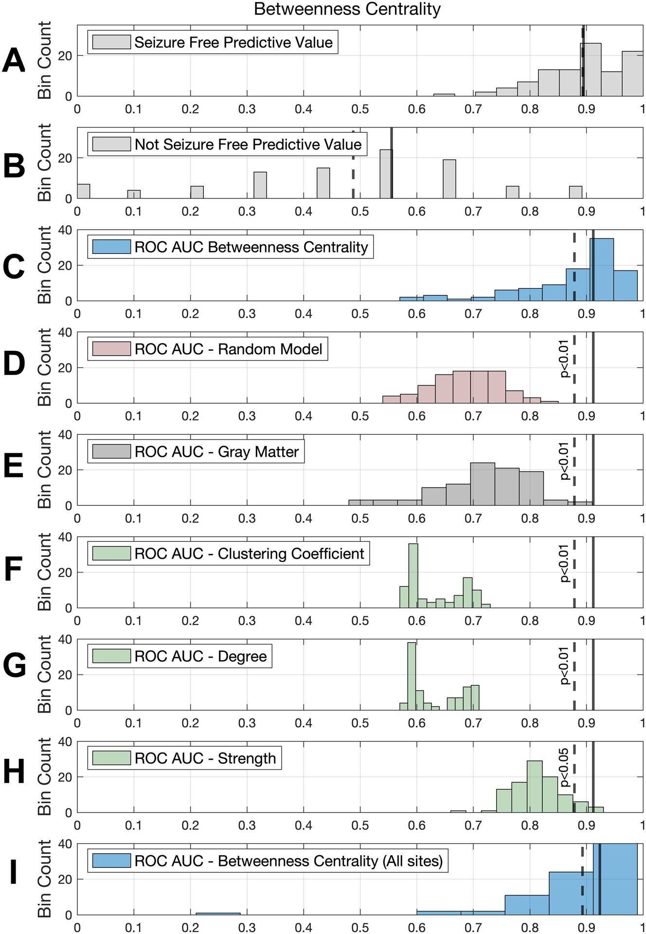
The top four rows show results for our top performing model: betweenness centrality. The distribution of predictive values with betweenness centrality is shown for (A) seizure free patients and (B) non-seizure free patients. Next, area under the curve (AUC) distributions are shown for betwenness centrality models (C) trained on real data and (D) trained on randomly shuffled data, which performed significantly worse than the former. Rows E-H show AUC distributions for the remainder of the models. In order to compare these with the top performing model, the continuous and dashed vertical lines in each row represent the median and mean, respectively, of the AUC for the betweenness centrality model and the p value indicates whether it was statistically significant, i.e., the probability that the other distribution would exhibit values higher than the average betweenness centrality AUC (see methods). Row I shows the betweenness centrality model with data from all sites used in training, with its corresponding mean and median AUCs.
Figure 3 summarizes the 15 regions with the highest importance on the classification model for betweenness centrality and whether the regional BC values were increased or decreased on SF vs NSF. The ROI with the highest importance was the parahippocampal gyrus ipsilateral to seizure onset, whose values were higher in the NSF patients. Overall, ROIs with the most importance involved both ipsilateral and contralateral regions in the medial and lateral temporal regions.
Figure 3.

Regional values with highest classification importance in the betweenness centrality model. The color code represents whether the average ROI was higher in patients who were non-seizure free (blue) vs. seizure free (red). Labels correspond to the AICHA atlas. Labels starting with ‘G’ correspond to gyri and ‘S’ correspond to sulci. ‘Ipsi’ and ‘Contra’ denote ROIs ipsilateral and contralateral to the side of seizure focus.
The anatomical distribution of classification importance can be seen on the left panel in Figure 4. The right panel of this same figure shows the T-values between SF and NSF groups. Note the higher group differences in medial and lateral temporal structures, notably with higher values in the medial ipsilateral structures. Yet, only some of the regions with higher between-group differences were important classification features in the out sample prediction machine learning model.
Figure 4.

The mosaic in the left panel illustrates feature importance regarding classification for the betweenness centrality model. Note the high importance of the ipsilateral parahippocampus, the contralateral superior temporal gyrus, and the bilateral entorhinal regions. The right panel demonstrates the t-values in the comparison of betweenness centrality values between seizure free (SF) and non-seizure free (NSF) groups. Positive values indicate higher values in the NSF group. In all coronal slices, the left side of the brain (i.e., the left temporal lobe in radiological convention) represents the side ipsilateral to seizure onset. Labels for ipsilateral (Ipsi) and contralateral (Contra) have been placed on the top right coronal slice of each panel for orientation purposes. Areas with stronger red coloring correspond to the most important (left panel) and most significantly different between the groups (right panel).
Discussion
In the present study, we sought to predict post-surgical outcomes based on data derived from the pre-surgical evaluation of patients with drug-resistant TLE. In particular, we focused on diffusion magnetic resonance imaging obtained pre-operatively at six different comprehensive epilepsy centers. Importantly, data from three of these centers were used to train machine learning models to be tested on a completely independent cohort of patients derived from the three remaining centers. By applying a single-layer feed-forward neural network classification model, we demonstrated that a measure of node hubness and network integration, namely betweenness centrality, could serve as a highly reliable source of individualized biomarkers in predicting which patients will be rendered fee from disabling seizures after epilepsy surgery. In particular, we found that changes to the integration of a subnetwork involving ipsilateral and contralateral medial and lateral temporal regions yielded very high accuracy for the prediction of seizure freedom after surgery.
Because of the complex nature of the structural connectome, mass univariate analyses (i.e., statistical tests applied independently for each regional connection) may suboptimally capture underlying changes in the global and local configuration of networks33. Our solution to this problem was two-fold. On the one hand, we focused on graph theory, which provides a mathematical framework to characterize different topological properties of a network’s organization. We have previously proposed that graph theory may show more consistency across scanners and across timepoints36 than mere link weights (i.e., values of connectivity strength between two given regions) and may reflect network changes otherwise undetected by mass univariate approaches33. One of the most fundamental concepts in graph theory is the balance between segregation (i.e., local connectivity) and integration (i.e., global network functioning). Centrality is a key measure of integration and it can be defined in several ways. BC in particular is computed based on the fraction of all shortest paths in the network that contain a given node. In other words, BC reflects the number of shortest paths from all nodes to all others that have to pass through a specific node. As such, a higher value of BC reflects the hubness of a node as an important, highly integrated influencer in the network. Structural connecitivty BC has been found to be one of the most relevant graph theory measures in differentiating other clinical populations including neuroinflammatory37, neuropsychiatric38, and neurodegenerative conditions39. We approached the analysis of graph theory measures from a temporal subnetwork using machine learning. With the concept that epilepsy is a network disorder, massive amounts of data need to be processed which may feature complex underlying patterns not otherwise detected by univariate algorithms. Naturally, this has led to an increased interest in applying machine learning algorithms, including artificial neural networks40.
Overall, our findings confirm the advantage of combining machine learning and graph theory in studying outcome phenotypes in epilepsy. The set of nodes that had the heaviest influence on the predictive models was in line with the brain regions that have been previously found to be critical in epilepsy patients across different modalities (e.g. in volume, cortical thickness, or structural and/or functional connectivity) relative to healthy populations9, 41–47. Here, it is key to note that there are several extra-temporal regions affected by TLE7, 48 which we did not probe as potential influencers of the predictive models. Their inclusion in the machine learning classifiers model could cause decreased accuracy due to overfitting. Therefore, to address the balance between meaningful regions and overfitting, without biasing the analyses on post-hoc results, we restricted the analyses to regions, predominantly temporal, previously defined in the literature as being most commonly affected in TLE49.
An important observation from our findings is the fact that predictive accuracy was driven by the model’s ability to correctly classify seizure-free patients. The performance for classification of non-seizure free status was suboptimal across all modalities tested. This finding has been previously seen in a single site study from our group that applied deep learning to whole-brain connectomics to predict post-operative seizure50. The present study further expanded these previous results in a number of different ways. First, we provide a multi-site approach that allowed for the reduction of biases associated with single center outcomes studies. This includes the fact that patients’ surgical eligibility was determined by different expert groups, different surgeries were performed at different sites and by different neurosurgeons, and follow-up outcome assessments were evaluated by different neurology teams, among others. We abated the potential for confounding effects introduced from the multi-site nature of this study by applying a well-established data harmonization approach validated for diffusion imaging29 and used in the well-established ENIGMA-Epilepsy consortium, which has previously pooled clinical imaging data from 24 research centers across 14 different countries9. Second, we focused on graph theory measures, demonstrating that a specific measure capable of reflecting nodal hubness is particularly reliable and significantly better than other graph theory measures that do not reflect the integration and segregation of the network, such as degree or strength of a node, or even clustering coefficient. In other words, we have demonstrated that the very high predictive accuracy of our model towards seizure freedom is not just the result of a reduced number of comparisons (that is, compared to entering thousands of region-to-region links weights as done in our previous study), else, other graph theory measures less reflective of network integration would have consistently yielded equally high predictive accuracy. Rather, the topological information conferred by a measure of betweenness centrality appears to capture information about the structural integration of the brain network in a way that it is predictive of post-surgical phenotyping. Therefore, the explanation for the suboptimal prediction of seizure refractoriness is likely multifactorial. In understanding the persistence of seizures, classification models may not be able to rely solely on structural- or diffusion-derived data alone. There is a possibility that combining different variables investigated in this study could have yielded improvements in classification, but the large number of possible combinations could have also led to overfitting. While the scope and goal of this study were to compare approaches for machine learning prediction as a first pass, these observations can be useful for future studies to build multimodal approaches without selection bias and with the inclusion of clinical variables.
Our findings must also be interpreted in the context of several caveats. We note that while Engel Class I does contemplate the possibility of focal seizures without loss of awareness following surgery, these patients are typically considered free of disabling seizures (i.e., with loss of consciousness). Future studies could explore the prediction of different degrees of non-seizure freedom in a more fine-grained manner. Along these lines, future studies should also contemplate the changes that occur over time for SF vs NSF status, which has been estimated to be 3–15% per year in either direction, although less so over time51. The retrospective nature of this study did not allow for collecting of seizure outcome status across different time points for all patients, so the analysis was performed using the one-year cut off commonly employed in outcome data of epilepsy surgery studies since the seminal Wiebe et al. controlled trial52. The retrospective nature of this study could have introduced biases inherent to this type of design. Importantly, the proportion of favorable to unfavorable outcomes did not appear to be associated with clinical site, side or type of surgery, and lesional vs. non-lesional cases.
Another potential limitation of studies using machine learning is the issue of cross-validation. Both relatively small samples or highly complex models could potentially lead to training overfitting, limiting the generalizability of the model. Here, we approached cross-validation via two gold standard different approaches. On the one hand, we tested models trained based on a multi-site cohort on a completely independent multi-site dataset. This means that the trained model was completely naïve to the testing data. In addition, we compared the model’s performance when trained on a randomly shuffled dataset; by doing so, the model was still trained on real data points, but ones that did not correspond to a naturally occurring combination/pattern.
Conclusions
To summarize, we have demonstrated that machine learning applied to betweenness centrality, a measure of network hubness computed from diffusion magnetic resonance imaging obtained during standard pre-surgical evaluation of patients with drug-resistant epilepsy, can be a highly accurate personalized biomarker to predict post-surgical outcomes in medial temporal lobe epilepsy, particularly seizure freedom status. High prediction accuracy based on betweenness centrality relative to other network properties likely reflects the biological mechanisms underlying widespread abnormal integration in brains with focal epilepsy. Thus, our findings confirm previous observations that topological changes occurring in medial and lateral temporal regions, both ipsilateral and contralateral to the presumed seizure focus, may be associated with distinct clinical phenotypes. Future studies using multicentric prospective designs, employing multi-modal approaches, and evaluating the influence of other clinical variables may help shed light on the complex mechanisms associated with such distinct post-surgical outcomes, especially seizure refractoriness. In doing so, the personalized diagnosis and management of epilepsy may help reduce current delays in surgical referral and alleviate the skepticism of both patients and healthcare providers in opting for surgery as an option to cure epilepsy.
Acknowledgments
This study was supported by grants from the National Institute of Neurological Disorders and Stroke (NINDS) 1R01NS110347-01A (LB, DLD, KAD, RK) and R21 NS107739 (LB, BM, CRM). SSK was supported by the UK Medical Research Council (MR/S00355X/1 and MR/K023152/1).
Footnotes
Potential Conflicts of Interest
The authors report no conflicts of interest related to this study.
References
- 1.Kramer MA, Cash SS. Epilepsy as a disorder of cortical network organization. The Neuroscientist : a review journal bringing neurobiology, neurology and psychiatry. 2012. August;18(4):360–72. [DOI] [PMC free article] [PubMed] [Google Scholar]
- 2.Cascino GD. Temporal lobe epilepsy: more than hippocampal pathology. Epilepsy currents / American Epilepsy Society. 2005. Sep-Oct;5(5):187–9. [DOI] [PMC free article] [PubMed] [Google Scholar]
- 3.Cohen-Gadol AA, Wilhelmi BG, Collignon F, et al. Long-term outcome of epilepsy surgery among 399 patients with nonlesional seizure foci including mesial temporal lobe sclerosis. Journal of neurosurgery. 2006. April;104(4):513–24. [DOI] [PubMed] [Google Scholar]
- 4.Engel J Jr., McDermott MP, Wiebe S, et al. Early surgical therapy for drug-resistant temporal lobe epilepsy: a randomized trial. JAMA : the journal of the American Medical Association. 2012. March 07;307(9):922–30. [DOI] [PMC free article] [PubMed] [Google Scholar]
- 5.Tellez-Zenteno JF, Wiebe S. Long-term seizure and psychosocial outcomes of epilepsy surgery. Curr Treat Options Neurol. 2008. July;10(4):253–9. [DOI] [PubMed] [Google Scholar]
- 6.Mohan M, Keller S, Nicolson A, et al. The long-term outcomes of epilepsy surgery. PloS one. 2018;13(5):e0196274. [DOI] [PMC free article] [PubMed] [Google Scholar]
- 7.Bonilha L, Rorden C, Castellano G, et al. Voxel-based morphometry reveals gray matter network atrophy in refractory medial temporal lobe epilepsy. Arch Neurol. 2004. September;61(9):1379–84. [DOI] [PubMed] [Google Scholar]
- 8.Bonilha L, Elm JJ, Edwards JC, et al. How common is brain atrophy in patients with medial temporal lobe epilepsy? Epilepsia. 2010. September;51(9):1774–9. [DOI] [PubMed] [Google Scholar]
- 9.Whelan CD, Altmann A, Botia JA, et al. Structural brain abnormalities in the common epilepsies assessed in a worldwide ENIGMA study. Brain : a journal of neurology. 2018. February 1;141(2):391–408. [DOI] [PMC free article] [PubMed] [Google Scholar]
- 10.Galovic M, van Dooren VQH, Postma T, et al. Progressive Cortical Thinning in Patients With Focal Epilepsy. JAMA Neurol. 2019. July 1. [DOI] [PMC free article] [PubMed] [Google Scholar]
- 11.Mehta A, Prabhakar M, Kumar P, Deshmukh R, Sharma PL. Excitotoxicity: bridge to various triggers in neurodegenerative disorders. Eur J Pharmacol. 2013. January 5;698(1–3):6–18. [DOI] [PubMed] [Google Scholar]
- 12.Bonilha L, Yasuda CL, Rorden C, et al. Does resection of the medial temporal lobe improve the outcome of temporal lobe epilepsy surgery? Epilepsia. 2007. March;48(3):571–8. [DOI] [PubMed] [Google Scholar]
- 13.Wu C, Jermakowicz WJ, Chakravorti S, et al. Effects of surgical targeting in laser interstitial thermal therapy for mesial temporal lobe epilepsy: A multicenter study of 234 patients. Epilepsia. 2019. June;60(6):1171–83. [DOI] [PMC free article] [PubMed] [Google Scholar]
- 14.Burns SP, Santaniello S, Yaffe RB, et al. Network dynamics of the brain and influence of the epileptic seizure onset zone. Proceedings of the National Academy of Sciences of the United States of America. 2014. December 9;111(49):E5321–30. [DOI] [PMC free article] [PubMed] [Google Scholar]
- 15.Khambhati AN, Davis KA, Oommen BS, et al. Dynamic Network Drivers of Seizure Generation, Propagation and Termination in Human Neocortical Epilepsy. PLoS computational biology. 2015. December;11(12):e1004608. [DOI] [PMC free article] [PubMed] [Google Scholar]
- 16.Parker CS, Clayden JD, Cardoso MJ, et al. Structural and effective connectivity in focal epilepsy. NeuroImage Clinical. 2018;17:943–52. [DOI] [PMC free article] [PubMed] [Google Scholar]
- 17.Olmi S, Petkoski S, Guye M, Bartolomei F, Jirsa V. Controlling seizure propagation in large-scale brain networks. PLoS computational biology. 2019. February;15(2):e1006805. [DOI] [PMC free article] [PubMed] [Google Scholar]
- 18.Kini LG, Bernabei JM, Mikhail F, et al. Virtual resection predicts surgical outcome for drug-resistant epilepsy. Brain : a journal of neurology. 2019. October 10. [DOI] [PMC free article] [PubMed] [Google Scholar]
- 19.Taylor PN, Sinha N, Wang Y, et al. The impact of epilepsy surgery on the structural connectome and its relation to outcome. NeuroImage Clinical. 2018;18:202–14. [DOI] [PMC free article] [PubMed] [Google Scholar]
- 20.Berg AT, Berkovic SF, Brodie MJ, et al. Revised terminology and concepts for organization of seizures and epilepsies: report of the ILAE Commission on Classification and Terminology, 2005–2009. Epilepsia. 2010. April;51(4):676–85. [DOI] [PubMed] [Google Scholar]
- 21.Engel J Jr., Wiebe S, French J, et al. Practice parameter: temporal lobe and localized neocortical resections for epilepsy. Epilepsia. 2003. June;44(6):741–51. [DOI] [PubMed] [Google Scholar]
- 22.Ashburner J, Friston KJ. Voxel-based morphometry--the methods. NeuroImage. 2000. June;11(6 Pt 1):805–21. [DOI] [PubMed] [Google Scholar]
- 23.Ashburner J, Csernansky JG, Davatzikos C, Fox NC, Frisoni GB, Thompson PM. Computer-assisted imaging to assess brain structure in healthy and diseased brains. Lancet neurology. 2003. February;2(2):79–88. [DOI] [PubMed] [Google Scholar]
- 24.Keller SS, Wilke M, Wieshmann UC, Sluming VA, Roberts N. Comparison of standard and optimized voxel-based morphometry for analysis of brain changes associated with temporal lobe epilepsy. NeuroImage. 2004. November;23(3):860–8. [DOI] [PubMed] [Google Scholar]
- 25.Joliot M, Jobard G, Naveau M, et al. AICHA: An atlas of intrinsic connectivity of homotopic areas. Journal of neuroscience methods. 2015. October 30;254:46–59. [DOI] [PubMed] [Google Scholar]
- 26.Hernandez M, Guerrero GD, Cecilia JM, et al. Accelerating fibre orientation estimation from diffusion weighted magnetic resonance imaging using GPUs. PloS one. 2013;8(4):e61892. [DOI] [PMC free article] [PubMed] [Google Scholar]
- 27.Behrens TE, Berg HJ, Jbabdi S, Rushworth MF, Woolrich MW. Probabilistic diffusion tractography with multiple fibre orientations: What can we gain? NeuroImage. 2007. Jan 1;34(1):144–55. [DOI] [PMC free article] [PubMed] [Google Scholar]
- 28.Johnson WE, Li C, Rabinovic A. Adjusting batch effects in microarray expression data using empirical Bayes methods. Biostatistics. 2007. January;8(1):118–27. [DOI] [PubMed] [Google Scholar]
- 29.Fortin JP, Parker D, Tunc B, et al. Harmonization of multi-site diffusion tensor imaging data. NeuroImage. 2017. November 1;161:149–70. [DOI] [PMC free article] [PubMed] [Google Scholar]
- 30.Hatton SN, Huynh KH, Bonilha L, et al. White matter abnormalities across different epilepsy syndromes in adults: an ENIGMA Epilepsy study. bioRxiv. 2019:2019.12.19.883405. [DOI] [PMC free article] [PubMed] [Google Scholar]
- 31.Rubinov M, Sporns O. Complex network measures of brain connectivity: uses and interpretations. NeuroImage. 2010. September;52(3):1059–69. [DOI] [PubMed] [Google Scholar]
- 32.Gleichgerrcht E, Kocher M, Bonilha L. Connectomics and graph theory analyses: Novel insights into network abnormalities in epilepsy. Epilepsia. 2015. November;56(11):1660–8. [DOI] [PubMed] [Google Scholar]
- 33.Bernhardt BC, Bonilha L, Gross DW. Network analysis for a network disorder: The emerging role of graph theory in the study of epilepsy. Epilepsy & behavior : E&B. 2015. July 6. [DOI] [PubMed] [Google Scholar]
- 34.Chawla NV, Bowyer KW, Hall LO, Kegelmeyer WP. SMOTE: Synthetic Minority Over-sampling Technique. Journal of Artificial Intelligence Research. 2002;16. [Google Scholar]
- 35.Del Gaizo J, Fridriksson J, Yourganov G, et al. Mapping Language Networks Using the Structural and Dynamic Brain Connectomes. eNeuro. 2017. Sep-Oct;4(5). [DOI] [PMC free article] [PubMed] [Google Scholar]
- 36.Bonilha L, Gleichgerrcht E, Fridriksson J, et al. Reproducibility of the Structural Brain Connectome Derived from Diffusion Tensor Imaging. PloS one. 2015;10(8):e0135247. [DOI] [PMC free article] [PubMed] [Google Scholar]
- 37.Zurita M, Montalba C, Labbe T, et al. Characterization of relapsing-remitting multiple sclerosis patients using support vector machine classifications of functional and diffusion MRI data. NeuroImage Clinical. 2018;20:724–30. [DOI] [PMC free article] [PubMed] [Google Scholar]
- 38.Thomas PJ, Panchamukhi S, Nathan J, et al. Graph theoretical measures of the uncinate fasciculus subnetwork as predictors and correlates of treatment response in a transdiagnostic psychiatric cohort. Psychiatry Res Neuroimaging. 2020 May 30;299:111064. [DOI] [PMC free article] [PubMed] [Google Scholar]
- 39.Ebadi A, Dalboni da Rocha JL, Nagaraju DB, et al. Ensemble Classification of Alzheimer’s Disease and Mild Cognitive Impairment Based on Complex Graph Measures from Diffusion Tensor Images. Frontiers in neuroscience. 2017;11:56. [DOI] [PMC free article] [PubMed] [Google Scholar]
- 40.Abbasi B, Goldenholz DM. Machine learning applications in epilepsy. Epilepsia. 2019. October;60(10):2037–47. [DOI] [PMC free article] [PubMed] [Google Scholar]
- 41.DeSalvo MN, Douw L, Tanaka N, Reinsberger C, Stufflebeam SM. Altered structural connectome in temporal lobe epilepsy. Radiology. 2014. March;270(3):842–8. [DOI] [PMC free article] [PubMed] [Google Scholar]
- 42.Dinkelacker V, Valabregue R, Thivard L, et al. Hippocampal-thalamic wiring in medial temporal lobe epilepsy: Enhanced connectivity per hippocampal voxel. Epilepsia. 2015. August;56(8):1217–26. [DOI] [PubMed] [Google Scholar]
- 43.Hermann B, Seidenberg M, Bell B, et al. Extratemporal quantitative MR volumetrics and neuropsychological status in temporal lobe epilepsy. Journal of the International Neuropsychological Society : JINS. 2003. March;9(3):353–62. [DOI] [PubMed] [Google Scholar]
- 44.McDonald CR, Ahmadi ME, Hagler DJ, et al. Diffusion tensor imaging correlates of memory and language impairments in temporal lobe epilepsy. Neurology. 2008. December 2;71(23):1869–76. [DOI] [PMC free article] [PubMed] [Google Scholar]
- 45.Seidenberg M, Kelly KG, Parrish J, et al. Ipsilateral and contralateral MRI volumetric abnormalities in chronic unilateral temporal lobe epilepsy and their clinical correlates. Epilepsia. 2005. March;46(3):420–30. [DOI] [PubMed] [Google Scholar]
- 46.Bonilha L, Lee CY, Jensen JH, et al. Altered microstructure in temporal lobe epilepsy: a diffusional kurtosis imaging study. AJNR American journal of neuroradiology. 2015. April;36(4):719–24. [DOI] [PMC free article] [PubMed] [Google Scholar]
- 47.Bonilha L, Nesland T, Martz GU, et al. Medial temporal lobe epilepsy is associated with neuronal fibre loss and paradoxical increase in structural connectivity of limbic structures. Journal of neurology, neurosurgery, and psychiatry. 2012. September;83(9):903–9. [DOI] [PMC free article] [PubMed] [Google Scholar]
- 48.Bernasconi N, Duchesne S, Janke A, Lerch J, Collins DL, Bernasconi A. Whole-brain voxel-based statistical analysis of gray matter and white matter in temporal lobe epilepsy. NeuroImage. 2004. October;23(2):717–23. [DOI] [PubMed] [Google Scholar]
- 49.Keller SS, Roberts N. Voxel-based morphometry of temporal lobe epilepsy: an introduction and review of the literature. Epilepsia. 2008. May;49(5):741–57. [DOI] [PubMed] [Google Scholar]
- 50.Gleichgerrcht E, Munsell B, Bhatia S, et al. Deep learning applied to whole-brain connectome to determine seizure control after epilepsy surgery. Epilepsia. 2018. September;59(9):1643–54. [DOI] [PubMed] [Google Scholar]
- 51.de Tisi J, Bell GS, Peacock JL, et al. The long-term outcome of adult epilepsy surgery, patterns of seizure remission, and relapse: a cohort study. Lancet. 2011. October 15;378(9800):1388–95. [DOI] [PubMed] [Google Scholar]
- 52.Wiebe S, Blume WT, Girvin JP, Eliasziw M, Effectiveness, Efficiency of Surgery for Temporal Lobe Epilepsy Study G. A randomized, controlled trial of surgery for temporal-lobe epilepsy. N Engl J Med. 2001. August 2;345(5):311–8. [DOI] [PubMed] [Google Scholar]