Scanning window analysis of non-coding regions within normal-tumor whole-genome sequence samples

Abstract

Genomics has benefited from an explosion in affordable high-throughput technology for whole-genome sequencing. The regulatory and functional aspects in non-coding regions may be an important contributor to oncogenesis. Whole-genome tumor-normal paired alignments were used to examine the non-coding regions in five cancer types and two races. Both a sliding window and a binning strategy were introduced to uncover areas of higher than expected variation for additional study. We show that the majority of cancer associated mutations in 154 whole-genome sequences covering breast invasive carcinoma, colon adenocarcinoma, kidney renal papillary cell carcinoma, lung adenocarcinoma and uterine corpus endometrial carcinoma cancers and two races are found outside of the coding region (4 432 885 in non-gene regions versus 1 412 731 in gene regions). A pan-cancer analysis found significantly mutated windows (292 to 3881 in count) demonstrating that there are significant numbers of large mutated regions in the non-coding genome. The 59 significantly mutated windows were found in all studied races and cancers. These offer 16 regions ripe for additional study within 12 different chromosomes—2, 4, 5, 7, 10, 11, 16, 18, 20, 21 and X. Many of these regions were found in centromeric locations. The X chromosome had the largest set of universal windows that cluster almost exclusively in Xq11.1—an area linked to chromosomal instability and oncogenesis. Large consecutive clusters (super windows) were found (19 to 114 in count) providing further evidence that large mutated regions in the genome are influencing cancer development. We show remarkable similarity in highly mutated non-coding regions across both cancer and race.

Introduction

High-throughput genomic sequencing technology has revolutionized biology [1, 2]. In the past, the non-coding region of the genome had been derided as junk DNA [3] or otherwise ignored [4]. More recently, regulatory and other functional aspects of non-coding DNA have been shown [5–9]. An example is the long non-coding RNA (lncRNA) MALAT-1’s involvement in the progression of colorectal cancer [10]. Hypermethylation of CpG islands associated with transcribed and ultra-conserved regions of DNA has been associated with various tumor types suggesting that non-coding RNAs can stabilize at least some subset of cell regulation [11]. Additional work has also pointed to the role of lncRNAs in cancer progression [12–17]. This body of work focused on known functional elements including lncRNAs, micro RNAs, enhancers and promotors. Other work has looked at regions beyond the exome but has not been extended to the whole genome systematically [18]. Examination of the non-coding region for cancer-associated variation bias could highlight currently unknown but functionally relevant DNA [19]. It stands to reason that at least some variations found within associated cancer tissue and not in normal adjacent tissue would be involved in the regulation or oncogenesis of that cancer.

We introduce a sliding window and binning approach in order to find windows in non-coding regions that are associated with five different cancer types. Due to the large amount of data found in the non-coding region of the genome, a window approach decreases the degrees of freedom of single nucleotide variation (SNV) analysis. Windows of interest in the genome are defined as 10k bases outside of the coding region with higher than expected mutations. We hypothesis that these windows, particularly universally occurring ones, provide an interesting opportunity for study. Further, we hypothesis that there are larger regions of these significantly mutated windows that can have a structural impact in oncogenesis or regulation.

Material and methods

Sample selection

For this study, a subsample of 154 samples were chosen for analysis over five different cancer types from The Cancer Genome Atlas (TCGA) whole-genome sequencing (WGS) tumor-normal paired data. Samples were chosen by filtering available data by both race and cancer. Five cancers were chosen: lung adenocarcinoma (LUAD), breast invasive carcinoma (BRCA), kidney renal papillary cell carcinoma (KIRP), uterine corpus endometrial carcinoma (UCEC) and colon adenocarcinoma (COAD). These specific cancers were chosen for several reasons. First, computational limitations required us to select a sample set smaller than the full scope of the data available. Second, lung, breast and colorectal are consistently ranked high in new cases. Third, we wanted a range in coverage within our data set—shown by fairly low sequencing coverage in COAD samples to much higher sequencing coverage in LUAD and BRCA samples in TCGA. Fourth, we needed cancer types that had enough white and African American samples in order to analyze, and this limited us significantly (Supplementary Table S1). See Supplementary Figure S1 for summary statistics on the raw data and Supplementary Table S1 for available samples in TCGA by race and cancer. (Additionally, there were roughly 20 samples additionally included in the study which had already had the variant call pipeline run for them from additional research. Since they were spread out among the five cancers and there was not identical numbers for each group, these were included them in the sample set for additional power in the analysis. They are included in the counts listed.) These samples were downloaded through dbGaP access in Google Cloud in collaboration with the Institute for Systems Biology, one of the projects making this type of data available to researchers in a cloud setting which provides a BigQuery table to retrieve access locations of specific data [20]. The exact TCGA IDs used are included in Supplementary Table S2.

Target samples sizes were determined by using the power formula:

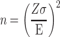Where Z represents a 95% confidence interval (1.96), σ was estimated by taking the standard deviation of TCGA VarScan samples somatic mutation counts in the TCGA data portal (~1212) [21] and setting the margin of error for raw count of cancer-associated SNVs to 200 since there was an expectation of sequencing artifacts in the pipeline. This formula can be used to estimate the power for a study with an estimate of the mean (average SNVs expected) of a continuous variable (number of SNVs can be thought of as continuous). The calculation result is that ~141 samples are needed to meet the goals of the study. The 154 final samples were used to hedge against some needed to be discarded for quality control purposes out of 161 targeted, exceeding the 141 predicted samples to give the study enough power. See Table 1 for final counts used in this study.

Table 1.

Final counts of paired samples by cancer and race. Final counts of paired samples broken down by both cancer and race. This table shows the number of samples examined in the final analysis after excluding outliers and other data that did not pass quality control checks. Orange bars represent visualizations of the number of relative samples within the same group while red bars represent the total scale of the cancer type within all samples

Variant calling

The SNV data set was then constructed from these samples. The alignment procedure from raw sequence data to BAM files was done by the TCGA network and is presented online [22]. Variant calling on normal-tumor pairs was then done through the TCGA VarScan2 pipeline performed in the Google Cloud Platform with custom scripts, see Figure 1.

Figure 1.

Variant calling pipeline from within Google Cloud. (A) Flowchart of the pipeline structure built in Google Cloud Engine. This required access to the TCGA data set hosted there as well as construction of a queuing system main node (Slurm was chosen), a variable series of computational nodes, a datastore to hold output data, an analytics database to track computations and a basic visualization system (web page) to inspect computation progress. Compute nodes were created using a custom Ubuntu image with appropriate bioinformatics and queuing software installed and configured. (B) Flowchart of the internal working on a single computational node. The main node submits a sample request to the computational node which then is able to parallelize the computation by splitting the BAM file and running the variant calling pipeline (panel C) in parallel. Information is saved to the analytics database, and output data is moved to the datastore. (C) Full pipeline for variant calling. This follows the canonical TCGA variant calling pipeline using VarScan as well as some custom metadata extraction and storage. (D) Pipeline of Manhattan plot generation pipeline for quality control metrics. Variant output files are downloaded from the datastore, file size is checked for quality control purposes, high confidence VCF files are extracted and indexed with tabix software. Variant calls per 10 000 base window are counted and used as the locations for plotting purposes and the counts are used as the y axis. Output data is arranged in the appropriate form and generated into Manhattan plots using R software.

BioCompute Object

BioCompute is a standardized format for the documentation of computational analyses. A computational workflow captured in this format is called a BioCompute Object (BCO). A BCO can be leveraged by the scientific community in lieu of traditional documentation as it captures the history and execution environment of the analysis, including any dependencies and prerequisites. A BCO therefore serves as documentation of provenance, substantially improves reproducibility and supports the generation of novel pipelines from existing workflows. More information on the BioCompute framework can be found online [23].

A BioCompute Object of the workflow developed in this paper is provided online [24].

Window generation

High confidence somatic SNV files were extracted and then indexed with the tabix [25] program. Windows were generated for each sample, as well as for pooled samples by cancer and race. The windows were 10 000 in base size to facilitate possible polymerase chain reaction (PCR) validation (email communications ThermoFisher Scientific). Pysam [26], pyvcf [27] and bespoke software were used to automate window calculations across all samples.

Windows were then plotted using a modified Manhattan plot. The x axis corresponded to the window by location and the y axis corresponded to the number of variations found within that window area. This was chosen in order to quickly visualize areas of the genome where there are significant clusters of variations. This quality control check was performed on each sample to look for inconsistencies due to failed computations. Visualizations are shown in Supplementary Figure S2.

Consensus coding region and gene masking

In addition to generating the above for the raw whole-genome output, consensus coding sequence regions were masked in order to focus on the non-coding region. These were chosen in order to focus on the non-coding region in line with the goals of this study. The CCDS track was used in the Genome Browser [28, 29] where the coding exons option was selected for the full genome. This output browser extensible data (BED) file was used with the bamstats [30, 31] tool to remove consensus CDS regions from the variant calling output from the WGS for samples in this study. Additionally, whole gene (Genome Browser, CCDS track, whole gene option) masking was also generated. These masking regions were more expansive than the CDS regions and included flanking gene features (5′ UTR, 3′ UTR, etc.) and introns.

Window hot spots

Next, the areas where there are ‘hot spots’ were examined. Hot spots are defined as 10k base regions where there were more variants found than were expected. The assumption for expected variations was that they would be found dispersed evenly throughout the genome in the non-coding region. This assumes that each part of the genome contributes to cellular function and regulation. Regions where there were significantly more variations than expected were extracted. Each pooled cancer/race pair was also examined in order to generate lists of highly mutated regions found across these grouped samples in a pan-cancer analysis.

In addition to raw values of counts (which lead to a bias for samples with extremely high coverage), a relative score for each window was calculated. The study employed a normalization strategy to weight the ‘value’ of a variant.

The normalization strategy used was:

Where is the number of SNVs in the current window, is the total number of SNVs in the sample, and is the total number of non-zero windows (windows that have at least one SNV). This analysis was run on individual sample levels for comparison purposes and then run on pooled sample levels for pan-cancer analysis.

Calculations of total variants in a sample were done with the bcftools [32] stats. The normalized top 20 windows were calculated for all results, all results by race and each cancer type by race.

Highly significant windows

Highly mutated regions found associated with race-specific cancer types were examined by looking at the pooled variants across each cancer. P-values were calculated for each window based on expected distribution of cancer-associated SNVs across the genome. The null hypothesis was that SNVs would be distributed equally throughout the genome. Regions where they cluster lead us to reject that hypothesis. P-values are shown as adjusted with the Bonferroni multiple testing correction.

Significance was calculated using the methodology described in [33] and in other work such as [34, 35]. This was based off of the statistics approach used in protein analysis through evolutionary relationships (PANTHER) pathway [36]. The P-values calculated represent the amount of deviance between a global ratio and an observed ratio in SNV counts and location. The calculation of the expected number of SNVs within a window region is shown below:

Calculating the expected variants is as follows:

Combining the previous two equations:

The probability of seeing a variation at a nucleotide site () was calculated by the total number of SNVs isolated and related to the cancer type (), divided by the size of the genome (G). The number of expected variants in a window () was calculated by taking the probably expected at a single position and multiplying it by the window size (). The expected number of sites, along with the observed number of sites, n_obs, was then used to calculate the P-value through the binomial statistic:

P-value scores that are shown as 0 are P-value << 10⁻⁵⁰. Highly mutated windows (adjusted P-values < 0.05) were pooled across all cancers and races.

Super windows

Regions where there were many windows over a short stretch of genome suggest that there may be 3D structural changes that have occurred. Isolating these stretches gives researchers the ability to narrow down on how chromosomes arrange themselves in the genome to understand better the regulatory effects of mutations there with respect to oncogenesis.

Significant windows were examined in aggregate for each gene-masked pooled sample (each race and cancer type). Gene-masked samples were chosen to remove coding and gene production regions in order to focus analysis on the non-coding portion of the DNA. All sets of windows in regions with no more than nine window gaps between them were brought together into a ‘super window’. This gave a size that is in line with an expansive view of a centimorgan as a unit of distance where the chromosomal crossover rate is around 0.01.

Results and discussion

Summary

The 154 variant call data sets were generated and examined out of approximately 2500 entries in TCGA. Entries in TCGA varied somewhat (see Supplementary Table S3) so this analysis was restricted to the pool of normal-tumor paired samples. Within that large data set, 154 samples were selected. Within those samples, 5 845 616 total cancer associated SNVs were identified across the whole genome for an average of about 37 958 SNVs per sample with a range of as low as 236 cancer-associated SNVs to as high as 484 464 cancer associated SNVs and a standard deviation of approximately 55 612. This suggests a wide range of sample preparation and read depth decisions particular for each experiment, as expected. When excluding the CDS, 5 821 577 cancer-associated SNVs were found with a minimum and maximum of 235 to 484 077 respectfully and a standard deviation of about 55 446. Lastly, when excluding consensus gene regions (including up- and downstream elements), a total of 4 432 885 cancer-associated SNVs ranging from 212 to 442 995 with a standard deviation of about 45 274 were found. The majority of cancer-associated SNVs fell outside of the coding region of the genome.

Manhattan style plots in Supplementary Figure S2 show evidence that there are larger regions with multiple proximate windows with high levels of SNVs. This suggests that these highly mutated areas are cancer associated since that is not expected that by chance [37–39]. These larger windows might represent larger regulatory structures such as three-dimensional positioning or other elements. Three-dimensional structural changes have been implicated in the cancer genome [40–43]. Cancer-specific three-dimensional structures have been found [44] and are potentially an important.

Window hotspots

SNV counts for a window were normalized and then calculated as described in the Methods section. Supplementary Tables S4 and S5 show three different analysis—raw high confident variant calls; high confident variant calls with CDS regions filtered out and high confidence variant calls with full gene regions filtered out for both analyzed races. Additionally, heat maps for individual samples clustered by cancer type and chromosome are given. Figure 2 shows the heat map of individual sample’s windows with gene structures masked while raw and CDS regions masked are shown in Supplementary Figure S3 and S4, respectively.

Figure 2.

Visualization of each sample w/ normalized counts when whole gene structure is masked: heat map of individual samples’ windows. SNVs within gene regions are masked and therefore removed from this analysis to focus on the non-coding region. SNV density of each window is shown in the color histogram key as normalized counts (normalized as described in the Methods section). Samples (X legend, right) are sorted by cancer type (Y legend, left) and clustered based on chromosome position (X legend, bottom) and chromosome (X legend, top). Dendrogram is based off of similarity of regions that are clustered (top). There is noticeable similarity on specific chromosome windows with high levels of SNV density across BRCA, LUAD and UCEC cancers. COAD and KIRP appear to have different footprints in this sample set versus the other cancers and each other. Clustering among this dimension (not shown) did not reveal any obvious pattern, however. Groups of windows with high levels of SNV density also cluster within each cancer group separately. This is the dimension clustered with the dendrogram and shows segments (specifically on the Y chromosome represented by the pink color in the top axis) where groups of windows with high density SNV counts appear across many if not all of the samples inter-cancer group. The Y chromosome group within KIRP has exceptionally consistent high SNV density that falls on a single chromosome suggesting an active and localized region of onco-related activity.

Looking at the heat map of individual samples, the most notable takeaway is a cluster of high variant windows clustered together in KIRP patients in the Y chromosome. This intriguing result deserves closer inspection in future study especially considering the (maybe controversial) role that the loss of Y chromosome has played in renal tumor classification [45].

Highly significant windows

A pan-cancer analysis was then done with variant data collected in this study. Normalized results for cancers pooled at the variant level and number of variants found in dbSNP are shown in Supplementary Table S6. Variant data among individuals with the same cancer designation and race were pooled into 10 comprehensive variant sets. These are grouped by cancer type and race pair—for full results, CDS masked and gene-masked—and are provided as Supplementary Table S4 and S5 (African American and White, respectively). The pooled data sets were then used to generate highly mutated windows of 10k bases. Counts of significantly mutated windows are show in Supplementary Table S7.

Universal highly significant windows. Within the data set, we found some windows that are found universally. There were 59 total 10k base windows that were found significantly mutated in all 10 race and cancer combinations (Figure 3, panel A). The windows were found in 12 different chromosomes—2, 4, 5, 7, 10, 11, 16, 18, 20, 21 and X. Visual representation is condensed due to the proximity of many of these windows to each other. A list of windows found across all cancers is in Supplementary Table S8. Figure 3, panel B shows a single chromosome—X—with 11 windows that cluster almost exclusively in Xq11.1, where the chromosome is divided by the centromere.

Figure 3.

Significantly mutated 10k base regions found in all race-cancer groupings. (A) visualization of significantly mutated 10k base regions throughout the genome. Chromosomes sizes are proportional to nucleotide length and shown in a circular plot with nucleotide position labels. Each orange bar marks a set of one or more significantly mutated 10k region (P < 0.05) that was found in all 10 cancer and race combinations in the location as labeled. Purple circles represent the average level of variant counts found in those marked regions and are proportional by size (as per the legend in the center of the diagram). Because of overlap, only the largest average in overlapping regions is visible (if a single orange line is representing five in close proximity, significantly mutated 10k regions, only the largest average variant count will be visible at the genome level). These regions exclude gene defined regions and are inclusive of significantly mutated 10k base regions that were found in all cancer and races. A total of 59 windows are shown, although many are clustered around each creating 16 distinct regions from a high-level view. (B) Zoomed in visualization of chromosome X, highlighting the additional windows found that are collapsed on the full genome visualization. Chromosome is shown in circular notation with significantly mutated 10k regions (P < 0.05) that were found across all 10 cancer and race combinations. This visualization shows that the 11 regions found highly mutated in Chromosome X are clustered into two proximate regions around base 60 000 000. (C) Number of 10k base regions found across all cancers and races with counts per chromosome (only chromosomes with at least one 10k window are shown). Chromosome X had the largest count although 12 chromosomes were represented. (D) Table view of the number of universal windows found for each chromosome.

In many of the chromosomes, we found that universal windows are either in the centromeric region or just outside of it. Other researchers have found that genetic instability can be associated with cancer, specific colorectal cancer [46, 47]. These have been mostly associated with gain or loss of whole chromosomes or regions of chromosomes [48]. Large scale mutation could also contribute to genetic instability in the same way that loss or rearrangement does. As shown with chromosome X, centromere instability could contribute to oncogenesis. Other research has found links between cancer and centromere-related proteins [49–53], centromere copy number variations [54] and chromosome instability [55, 56]. With this in mind, regions of these highly impacted chromosomes offer ample opportunity for study.

Due to their universal appearance, these regions are the strongest candidates for research to see if they are drivers in cancer. Chromosomes 4, 11, 16 and X show the highest numbers of highly mutated window counts across all groups as shown in Figure 3, panels C and D. We also show in Supplementary Table S8 that these regions are found more often than expected using a binomial test. This is true in 11 different chromosomes after adjusting for multiple testing, with the exception being chromosome 18.

Additionally, Figure 4 shows a more detailed breakdown of the regions that the highly mutated windows reside in. Shown are the affected chromosomes. Each cluster of windows is shown in a zoomed-in window of the region in the associated boxes. P-value indicators are by each chromosome label for whether or not the universal windows in that chromosome were found in centromere regions more often than expected using a binomial test.

Figure 4.

Universal window locations with normalized variant counts. Universal windows are shown across the affected chromosomes here. Giemsa staining regions are also shown, including red regions representing the centromeric regions. Sections of super windows are drawn out for each chromosome. For each of the zoomed in regions, the individual super windows are shown (they are typically clustered, with a few exceptions) with the individual super windows height representing the variation level. These are drawn proportionally across all chromosomes, even though the zoomed region is of different base length size in a few of the illustrations. As shown, many of the super windows across the genome (a strong majority) fall within the centromeric regions or are proximate to them.

Conservation of the universal windows was also looked at in Supplementary Figure S5. The phyloP46Way data set was retrieved from http://hgdownload.cse.ucsc.edu/goldenPath/hg19/phyloP46way/primates/ for primates and the universal windows individual bases were annotated with it. Supplementary Table S9 includes the scores by individual positions. A number of the universal windows are shown to have positive phyloP scores that suggest slower evolution than expected. This conservation is indicative of these regions having some function that could be related to oncogenesis. Conservation in these regions track with the hypothesis that these highly mutated regions found in cancer have some type of structural or otherwise functional impact on the cell. Many of the universal windows lack overlap with conserved regions and suggest that there may be different methods of impact that these windows have on oncogenesis. It is possible that the mechanism of action varies by window and this analysis helps to categorize some of these windows for further study.

Validation

Although the non-coding region is understudied, we were able to validate the results by examining the 59 universally found windows. Given that these regions are highly mutated with cancer associated variants, we believe that at least some of them should show known cancer variations. To examine this, we compared against the COSMIC database’s non-coding variants [57]. We found a majority—31—of the universal windows carried multiple known cancer-associated variants (Supplementary Table S10).

In addition, we examined the regions individually and found supporting evidence for many of them. Windows in 2q21 have been linked to oxyphilic tumors, specifically through loss of heterozygosity [58] and in non-medullary thyroid carcinoma [59]. 3p12.3 also has reported loss of heterozygosity (LOH) associated with lung and other malignancies [60]. 3p11 and 3p12 regions have multiple genetic pathways that are known to amplify various tumors through increased expression of VGLL3 and CHMP2B [61]. 4q35.2 analysis has shown long range interactions related to disease [62] and the region has shown hypersensitivity to DNase I [63]. This region has also been linked to acute myeloid leukemia [64]. 7p11.2 has features that have been found in numerous cancers [65]. There are also breakpoint enriched differentially methylated regions directly upstream of EGFR and HIPI [66]. 11p11.12 has been shown to be linked to esophageal squamous cell carcinoma [67] and linkage in the region was shown for families suffering from primary renal cell carcinoma [68]. This survey of known associations related to these windows provides an additional validation that the technique used can be successful in narrowing down regions of interest.

Finally, we examined whether or not the clinical outcome could be predicted with either the number of universal windows found in a particular sample or the total cancer-associated variants found within these windows. The clinical outcome chosen was vital status that is coded as either 0 (deceased) or 1 (alive). A logistic regression was run to test their correlation with controlling for cancer type. The results can be found in Supplementary Table S11. The number of variants in these windows does not appear to have predictive power, but the number of universal windows an individual has mutated might. This validation provides additional evidence that the sliding window method can help determine non-coding hot-spots in cancer.

Super windows

Gene-masked super windows with an overrepresentation of SNVs were generated. This information gives some indication of highly impacted regions at a higher level than the window level. Figure 5 shows the overlay between the two races examined for each cancer type with Giemsa staining regions highlighted while Supplementary Table S12 shows the counts for each race broken down by cancer type.

Figure 5.

Overlaps of super windows between race for each cancer type for gene-masked results. Display of super windows overlap between races for each cancer type. Red represents African American super windows while blue represents White super windows. Super windows are defined as regions where there were statistically significant levels of mutations for stretches of 10k base windows within 10 windows of each other with a minimum of four windows in a stretch. Chromosomes are shown with Giemsa staining regions highlighted. This shows heterochromatic regions staining more darkly depending on how condensed and AT rich they are. These regions are typically gene poor. Gene rich euchromatin regions, on the other hand, are stained lightly or not at all. These regions are typically more transcriptionally active and often associated with the gene coding regions of the genome. Since gene regions have been masked in the super window regions, we anticipate a higher proportion of windows in the stained regions—which is what is seen. The red coloring specifically shows the centromeric regions (for illustration, this does not map to the staining results). There are notable visual similarities in where these highly mutated regions fall, not only within both races for many of them, but even between cancer types themselves suggesting some common areas of structural mutation related to oncogenesis.

When looking at the visualizations in Figure 5, there is remarkable overlap of regions between the two races both within cancer and across all cancers. There are some notable differences that offer opportunity for further study since it has been observed that race-related mutational differences can have clinical implications [69, 70]. It is also possible that some of these results are related to data irregularities. For example, there is a region towards the beginning of chromosome 1 that is found in both African American and White pooled samples in BRCA, KIRP and UCEC. In COAD, it is only in the African American pooled sample while in LUAD, it is only found in the White sample. Given the regularity across the other samples, this may be a data issue in both COAD and LUAD. However, chromosome Y shows regions that appear similar as well as ones that are not consistent across the various cancers. This is particularly noticeable in the super window region in KIRP for this chromosome, matching the individual sample analysis above where Y chromosome windows were clustered together in these patients.

Conclusion

We generated a large variant pool of high confidence cancer-associated single nucleotide variations for analysis genome wide, excluding CDS regions, and finally excluding entire gene regions. This data was shared with the Institute for Systems Biology and is accessible to dbGaP authenticated researchers on their cancer cloud installation. Our focus was on the non-coding region of the genome. This analysis was run on a cluster of computers on Google Cloud Engine in association with the NIH Cancer Cloud Pilot. We found that there is a wide variety of variants over individual samples likely due to both differences in read depth and sample preparation since the samples themselves were prepared in a number of partner labs. We also found that the vast majority of the cancer-associated mutations fell outside of the gene coding regions suggesting a widely understudied plethora of genetic variation in cancer samples.

Windows throughout the genome of size 10 000 bases were generated and then analyzed for overrepresentation of variations. We found that within KIRP there are a number of highly mutated windows in the Y chromosome that were consistent across samples. Pooling together the variants into a pan-cancer analysis allowed us to further look at the mutation profile from a higher level than the sample level. Significant windows that were found universally in all cancers and races are predominantly clustered near the centromeric regions on about half of human chromosomes suggesting that centromere stability may have a role in cell dis-regulation. Many of the same super regions (regions of high numbers of significantly varied windows) are in similar locations between both races and even between cancer types—with some notable exceptions.

Together, these results suggest that the non-coding region of the genome offers rich opportunity for discovery of different pathways that contribute to oncogenesis due to its complex disease status. They also suggest that cancer-associated mutations are mostly indistinguishable between African Americans and White Americans with some possible exceptions that could lead to exciting discoveries in personalized medicine.

Key Points

• A sliding window analysis done of whole-genome sequences showed that large numbers of 10k base pair windows in the non-coding regions of the genome exhibit highly significant mutations in different cancers.

• The 59 of these windows were found universally across all cancers and races examined in this study and were found to cluster in general around the centromeric region.

• The use of this technique shows an approach that can help understand large amounts of genomics data, such as that found in the non-coding region of the genome.

John Torcivia is a PhD candidate at the George Washington University in genomics and bioinformatics whose research focuses on the non-coding region of the genome and cancer formation.

Raja Mazumder is a professor in the Department of Biochemistry and Molecular Medicine and co-director of the McCormick Genomic and Proteomic Center at the George Washington University.

Availability

The data sets generated and/or analyzed during the current study are not publicly available due restricted access to whole-genome TCGA data but are available from the corresponding author on reasonable request. The variant call data has been ingested by the Institute for Systems Biology to be made available for authorized researchers both through BigQuery and as raw VCF files.

Funding

This project has been funded in part with Federal funds from the National Cancer Institute, National Institutes of Health, under contract no. HHSN261200800001E. This funding to the Institute for System’s Biology indirectly funded this research. Partly funded by National Cancer Institute grant no. U01CA215010 to R.M.

Disclosure

The authors have declared no conflicts of interest.

References

- 1. Delseny M, Han B, Hsing YI. High throughput DNA sequencing: the new sequencing revolution. Plant Sci 2010;179:407–22. [DOI] [PubMed] [Google Scholar]
- 2. Koboldt DC, Steinberg KM, Larson DE, et al. The next-generation sequencing revolution and its impact on genomics. Cell 2013;155:27–38. [DOI] [PMC free article] [PubMed] [Google Scholar]
- 3. Doolittle WF. Is junk DNA bunk? A critique of ENCODE. Proc Natl Acad Sci 2013;5294–5300. [DOI] [PMC free article] [PubMed] [Google Scholar]
- 4. Palazzo AF, Gregory TR. The case for junk DNA. PLoS Genet 2014;10:e1004351. [DOI] [PMC free article] [PubMed] [Google Scholar]
- 5. Pennisi E. Genomics. ENCODE project writes eulogy for junk DNA. Science 2012;1159(1161):337. [DOI] [PubMed] [Google Scholar]
- 6. Biémont C, Genetics VC. Junk DNA as an evolutionary force. Nature 2006;443:521. [DOI] [PubMed] [Google Scholar]
- 7. Nowak R. Mining treasures from ‘junk DNA’. (includes related glossary). Science 1994;263:608–11. [DOI] [PubMed] [Google Scholar]
- 8. Willingham AT, Gingeras TR. TUF love for ‘junk’ DNA. Cell 2006;125:1215–20. [DOI] [PubMed] [Google Scholar]
- 9. Ling H, Vincent K, Pichler M, et al. Junk DNA and the long non-coding RNA twist in cancer genetics. Oncogene 2015;34:5003. [DOI] [PMC free article] [PubMed] [Google Scholar]
- 10. Xu C, Yang M, Tian J, et al. MALAT-1: a long non-coding RNA and its important 3′ end functional motif in colorectal cancer metastasis. Int J Oncol 2011;39:169–75. [DOI] [PubMed] [Google Scholar]
- 11. Lujambio A, Portela A, Liz J, et al. CpG island hypermethylation-associated silencing of non-coding RNAs transcribed from ultraconserved regions in human cancer. Oncogene 2010;29:6390. [DOI] [PMC free article] [PubMed] [Google Scholar]
- 12. Mitra SA, Mitra AP, Triche TJ. A central role for long non-coding RNA in cancer. Front Genet 2012;3:17. [DOI] [PMC free article] [PubMed] [Google Scholar]
- 13. Tano K, Akimitsu N. Long non-coding RNAs in cancer progression. Front Genet 2012;3:219. [DOI] [PMC free article] [PubMed] [Google Scholar]
- 14. Merry CR, Forrest ME, Sabers JN, et al. DNMT1-associated long non-coding RNAs regulate global gene expression and DNA methylation in colon cancer. Hum Mol Genet 2015;24:6240–53. [DOI] [PMC free article] [PubMed] [Google Scholar]
- 15. Endo H, Shiroki T, Nakagawa T, et al. Enhanced expression of long non-coding RNA HOTAIR is associated with the development of gastric cancer. PloS One 2013;8:e77070. [DOI] [PMC free article] [PubMed] [Google Scholar]
- 16. Akrami R, Jacobsen A, Hoell J, et al. Comprehensive analysis of long non-coding RNAs in ovarian cancer reveals global patterns and targeted DNA amplification. PloS One 2013;8:e80306. [DOI] [PMC free article] [PubMed] [Google Scholar]
- 17. Prensner JR, Chinnaiyan AM. The emergence of lncRNAs in cancer biology. Cancer Discov 2011;1:391–407. [DOI] [PMC free article] [PubMed] [Google Scholar]
- 18. Araya CL, Cenik C, Reuter JA, et al. Identification of significantly mutated regions across cancer types highlights a rich landscape of functional molecular alterations. Nat Genet 2016;48:117. [DOI] [PMC free article] [PubMed] [Google Scholar]
- 19. Nakagawa H, Fujita M. Whole genome sequencing analysis for cancer genomics and precision medicine. Cancer Sci 2018;109:513–22. [DOI] [PMC free article] [PubMed] [Google Scholar]
- 20. Reynolds SM, Miller M, Lee P, et al. The ISB Cancer Genomics Cloud: a flexible cloud-based platform for cancer genomics research. Cancer Res 2017;77:e7–10. [DOI] [PMC free article] [PubMed] [Google Scholar]
- 21. GDC . GDC portal. https://portal.gdc.cancer.gov/exploration.
- 22. GDC . DNA-Seq analysis. https://docs.gdc.cancer.gov/Data/Bioinformatics_Pipelines/DNA_Seq_Variant_Calling_Pipeline/.
- 23. Partnership B. BioCompute specification. http://biocomputeobject.org/.
- 24. Torcivia J. Biocompute object describing this research. https://github.com/syntheticgio/bco_wgs_varscan_analysis.
- 25. Li H. Tabix: fast retrieval of sequence features from generic TAB-delimited files. Bioinformatics 2011;27:718–9. [DOI] [PMC free article] [PubMed] [Google Scholar]
- 26. Pysam-developers . Pysam. https://github.com/pysam-developers/pysam.
- 27. Casbon J. PyVCF. https://github.com/jamescasbon/PyVCF.
- 28. Kent WJ, Sugnet CW, Furey TS, et al. The human genome browser at UCSC. Genome Res 2002;12:996–1006. [DOI] [PMC free article] [PubMed] [Google Scholar]
- 29. Fujita PA, Rhead B, Zweig AS, et al. The UCSC genome browser database: update 2011. Nucleic Acids Res 2010;39:D876–82. [DOI] [PMC free article] [PubMed] [Google Scholar]
- 30. Afgan E, Baker D, Van den Beek M, et al. The galaxy platform for accessible, reproducible and collaborative biomedical analyses: 2016 update. Nucleic Acids Res 2016;44:W3–10. [DOI] [PMC free article] [PubMed] [Google Scholar]
- 31. Afgan E, Baker D, Batut B, et al. The galaxy platform for accessible, reproducible and collaborative biomedical analyses: 2018 update. Nucleic Acids Res 2018;46:W537–44. [DOI] [PMC free article] [PubMed] [Google Scholar]
- 32. Li H, Handsaker B, Wysoker A, et al. The sequence alignment/map format and SAMtools. Bioinformatics 2009;25:2078–9. [DOI] [PMC free article] [PubMed] [Google Scholar]
- 33. Karagiannis K, Simonyan V, Mazumder R. SNVDis: a proteome-wide analysis service for evaluating nsSNVs in protein functional sites and pathways. Genom Proteom Bioinf 2013;11:122–6. [DOI] [PMC free article] [PubMed] [Google Scholar]
- 34. Pan Y, Karagiannis K, Zhang H, et al. Human germline and pan-cancer variomes and their distinct functional profiles. Nucleic Acids Res 2014;42:11570–88. [DOI] [PMC free article] [PubMed] [Google Scholar]
- 35. Pan Y, Yan C, Hu Y, et al. Distribution bias analysis of germline and somatic single-nucleotide variations that impact protein functional site and neighboring amino acids. Sci Rep 2017;7:42169. [DOI] [PMC free article] [PubMed] [Google Scholar]
- 36. Mi H, Thomas P. PANTHER pathway: an ontology-based pathway database coupled with data analysis tools. Methods Mol Biol 2009;563:123–40. [DOI] [PMC free article] [PubMed] [Google Scholar]
- 37. Weinhold N, Jacobsen A, Schultz N, et al. Genome-wide analysis of noncoding regulatory mutations in cancer. Nat Genet 2014;46:1160. [DOI] [PMC free article] [PubMed] [Google Scholar]
- 38. Roberts SA, Sterling J, Thompson C, et al. Clustered mutations in yeast and in human cancers can arise from damaged long single-strand DNA regions. Mol Cell 2012;46:424–35. [DOI] [PMC free article] [PubMed] [Google Scholar]
- 39. Tamborero D, Gonzalez-Perez A, Lopez-Bigas N. OncodriveCLUST: exploiting the positional clustering of somatic mutations to identify cancer genes. Bioinformatics 2013;29:2238–44. [DOI] [PubMed] [Google Scholar]
- 40. Fudenberg G, Getz G, Meyerson M, et al. High order chromatin architecture shapes the landscape of chromosomal alterations in cancer. Nat Biotechnol 2011;29:1109. [DOI] [PMC free article] [PubMed] [Google Scholar]
- 41. Taberlay PC, Achinger-Kawecka J, Lun AT, et al. Three-dimensional disorganization of the cancer genome occurs coincident with long-range genetic and epigenetic alterations. Genome Res 2016;26:719–31. [DOI] [PMC free article] [PubMed] [Google Scholar]
- 42. Corces MR, Corces VG. The three-dimensional cancer genome. Curr Opin Genet Dev 2016;36:1–7. [DOI] [PMC free article] [PubMed] [Google Scholar]
- 43. Hnisz D, Schuijers J, Li CH, et al. Regulation and dysregulation of chromosome structure in cancer. Annu Rev Cancer Biol 2018;2:21–40. [Google Scholar]
- 44. Achinger-Kawecka J, Taberlay PC, Clark SJ. Alterations in three-dimensional organization of the cancer genome and epigenome. In: Cold Spring Harbor Symposia on Quantitative Biology. Cold Spring Harbor, NY: Cold Spring Harbor Laboratory Press, 2016, 41–51. [DOI] [PubMed] [Google Scholar]
- 45. Lopez-Beltran A, Scarpelli M, Montironi R, et al. 2004 WHO classification of the renal tumors of the adults. Eur Urol 2006;49:798–805. [DOI] [PubMed] [Google Scholar]
- 46. Lengauer C, Kinzler KW, Vogelstein B. Genetic instability in colorectal cancers. Nature 1997;386:623. [DOI] [PubMed] [Google Scholar]
- 47. Albertson DG, Collins C, McCormick F, et al. Chromosome aberrations in solid tumors. Nat Genet 2003;34:369. [DOI] [PubMed] [Google Scholar]
- 48. Geigl JB, Obenauf AC, Schwarzbraun T, et al. Defining ‘chromosomal instability’. Trends Genet 2008;24:64–9. [DOI] [PubMed] [Google Scholar]
- 49. Tomonaga T, Matsushita K, Yamaguchi S, et al. Overexpression and mistargeting of centromere protein-A in human primary colorectal cancer. Cancer Res 2003;63:3511–6. [PubMed] [Google Scholar]
- 50. Tomonaga T, Matsushita K, Ishibashi M, et al. Centromere protein H is up-regulated in primary human colorectal cancer and its overexpression induces aneuploidy. Cancer Res 2005;65:4683–9. [DOI] [PubMed] [Google Scholar]
- 51. Nakamura Y, Tanaka F, Haraguchi N, et al. Clinicopathological and biological significance of mitotic centromere-associated kinesin overexpression in human gastric cancer. Br J Cancer 2007;97:543. [DOI] [PMC free article] [PubMed] [Google Scholar]
- 52. McGovern SL, Qi Y, Pusztai L, et al. Centromere protein-A, an essential centromere protein, is a prognostic marker for relapse in estrogen receptor-positive breast cancer. Breast Cancer Res 2012;14:R72. [DOI] [PMC free article] [PubMed] [Google Scholar]
- 53. Bieniek J, Childress C, Swatski MD, et al. COX-2 inhibitors arrest prostate cancer cell cycle progression by down-regulation of kinetochore/centromere proteins. Prostate 2014;74:999–1011. [DOI] [PubMed] [Google Scholar]
- 54. Jang MH, Kim EJ, Kim HJ, et al. Assessment of HER2 status in invasive breast cancers with increased centromere 17 copy number. Breast Cancer Res Treat 2015;153:67–77. [DOI] [PubMed] [Google Scholar]
- 55. Rodriguez J, Frigola J, Vendrell E, et al. Chromosomal instability correlates with genome-wide DNA demethylation in human primary colorectal cancers. Cancer Res 2006;66:8462–9468. [DOI] [PubMed] [Google Scholar]
- 56. Kondo Y, Shen L, Ahmed S, et al. Downregulation of histone H3 lysine 9 methyltransferase G9a induces centrosome disruption and chromosome instability in cancer cells. PloS One 2008;3:e2037. [DOI] [PMC free article] [PubMed] [Google Scholar]
- 57. Tate JG, Bamford S, Jubb HC, et al. COSMIC: the catalogue of somatic mutations in cancer. Nucleic Acids Res 2019;47:D941–7. [DOI] [PMC free article] [PubMed] [Google Scholar]
- 58. Stankov K, Pastore A, Toschi L, et al. Allelic loss on chromosomes 2q21 and 19p 13.2 in oxyphilic thyroid tumors. Int J Cancer 2004;111:463–7. [DOI] [PubMed] [Google Scholar]
- 59. Prazeres HJ, Rodrigues F, Soares P, et al. Loss of heterozygosity at 19p13. 2 and 2q21 in tumours from familial clusters of non-medullary thyroid carcinoma. Fam Cancer 2008;7:141–9. [DOI] [PubMed] [Google Scholar]
- 60. Angeloni D, ter Elst A, Wei MH, et al. Analysis of a new homozygous deletion in the tumor suppressor region at 3p12. 3 reveals two novel intronic noncoding RNA genes. Genes Chromosomes Cancer 2006;45:676–91. [DOI] [PubMed] [Google Scholar]
- 61. Hallor KH, Sciot R, Staaf J, et al. Two genetic pathways, t (1; 10) and amplification of 3p11–12, in myxoinflammatory fibroblastic sarcoma, haemosiderotic fibrolipomatous tumour, and morphologically similar lesions. J Pathol 2009;217:716–27. [DOI] [PubMed] [Google Scholar]
- 62. Gaillard M-C, Broucqsault N, Morere J, et al. Analysis of the 4q35 chromatin organization reveals distinct long-range interactions in patients affected with Facio-Scapulo-humeral dystrophy. Sci Rep 2019;9:1–15. [DOI] [PMC free article] [PubMed] [Google Scholar]
- 63. Xu X, Tsumagari K, Sowden J, et al. DNaseI hypersensitivity at gene-poor, FSH dystrophy-linked 4q35. 2. Nucleic Acids Res 2009;37:7381–93. [DOI] [PMC free article] [PubMed] [Google Scholar]
- 64. Pession A, Nigro LL, Montemurro L, et al. ArgBP2, encoding a negative regulator of ABL, is fused to MLL in a case of infant M5 acute myeloid leukemia involving 4q35 and 11q23. Leukemia 2006;20:1310–3. [DOI] [PubMed] [Google Scholar]
- 65. Schaad K, Strömbeck B, Mandahl N, et al. FISH mapping of i (7q) in acute leukemias and myxoid liposarcoma reveals clustered breakpoints in 7p11. 2: implications for formation and pathogenetic outcome of the idic (7)(p11. 2). Cytogenet Genome Res 2006;114:126–30. [DOI] [PubMed] [Google Scholar]
- 66. Tang M-HE, Varadan V, Kamalakaran S, et al. Major chromosomal breakpoint intervals in breast cancer co-localize with differentially methylated regions. Front Oncol 2012;2:197. [DOI] [PMC free article] [PubMed] [Google Scholar]
- 67. Brown J, Bothma H, Veale R, et al. Genomic imbalances in esophageal carcinoma cell lines involve Wnt pathway genes. World J Gastroenterol: WJG 2011;17:2909. [DOI] [PMC free article] [PubMed] [Google Scholar]
- 68. Johanneson B, Deutsch K, McIntosh L, et al. Suggestive genetic linkage to chromosome 11p11. 2-q12. 2 in hereditary prostate cancer families with primary kidney cancer. Prostate 2007;67:732–42. [DOI] [PubMed] [Google Scholar]
- 69. Kurian AW. BRCA1 and BRCA2 mutations across race and ethnicity: distribution and clinical implications. Curr Opin Obstet Gynecol 2010;22:72–8. [DOI] [PubMed] [Google Scholar]
- 70. Greenup R, Buchanan A, Lorizio W, et al. Prevalence of BRCA mutations among women with triple-negative breast cancer (TNBC) in a genetic counseling cohort. Ann Surg Oncol 2013;20:3254–8. [DOI] [PubMed] [Google Scholar]
Associated Data
This section collects any data citations, data availability statements, or supplementary materials included in this article.