Compressed sensing for highly efficient imaging transcriptomics

Abstract

Recent methods for spatial imaging of tissue samples can identify up to ~100 individual proteins^1–3 or RNAs^4–10 at single-cell resolution. However, the number of proteins or genes that can be studied in these approaches is limited by long imaging times. Here, we introduce Composite In Situ Imaging (CISI), a method that leverages structure in gene expression across both cells and tissues to limit the number of imaging cycles needed to obtain spatially resolved gene expression maps. CISI defines gene modules that can be detected using composite measurements from imaging probes for subsets of genes. The data are then decompressed to recover expression values for individual genes. CISI further reduces imaging time by not relying on spot-level resolution, enabling lower magnification acquisition, and is overall about 500-fold more efficient than current methods. Applying CISI to 12 mouse brain sections, we accurately recovered the spatial abundance of 37 individual genes from 11 composite measurements covering 180 mm² and 476,276 cells.

Most current highly multiplexed methods for imaging RNA are based on single-molecule fluorescence in situ hybridization (smFISH)¹¹, with rounds of staining and stripping, and various barcoding strategies to increase multiplexing^4–10. In “linear” barcoding (e.g., osmFISH⁹ or in situ HCR¹⁰), each color in each round corresponds to one gene. The number of genes G that can be measured with c colors and r rounds is thus G = cr. In “combinatorial” strategies, such as MERFISH^4,8 or Seq-FISH^5,6, gene identity is encoded by a sequence of colors over multiple rounds, such that G = 2^rc −1 genes can be measured with c colors (typically 1–4) and r rounds (ignoring additional rounds needed for error correction). Such multiplex methods have provided an unprecedented tool for tissue biology and histopathology, but they typically measure fewer than 1% of genes, necessitate choosing a gene-expression signature, and can require a week or more to collect data in a single tissue section. Ideally, it would be possible to quickly generate data on thousands of gene abundance levels in large tissue volumes, perhaps even entire organs.

Because existing barcoding methods ignore prior knowledge or biological principles, each spot is decoded independently, leading to two fundamental limitations on scalability. First, quantification requires imaging at high magnification (up to 100x) so that individual RNA molecules appear as bright, well-separated spots. High-resolution image acquisition over large volumes is slow. Second, there are limitations on the number of genes. In linear barcoding, it is not feasible to substantially increase the number G of genes assayed, because the number of rounds of imaging scales with G; in combinatorial barcoding, increases are limited by optical crowding (spatial overlap between fluorescent spots), because the number of spots scales with G. Recent efforts to ameliorate this issue with sparser combinatorial barcodes increase the number of rounds of hybridization and, so far, result in a relatively high rate of false positives¹².

We reasoned that a strategy informed by biological principles of gene expression patterns could be more efficient. As we have previously shown theoretically¹³ , when genes are co-regulated, one might infer the expression of many individual genes from a much smaller number of composite measurements of abundance – mathematically defined as linear combinations of gene abundance levels – consisting of combined signal from multiple genes on the same channel. We have previously described how the theoretical foundations of this strategy, based on the mathematics of compressed sensing¹³, enables under-sampled composite data to be decompressed to recover structured, high-dimensional expression for individual genes.

Here, we develop such a scheme, Composite In Situ Imaging (CISI), implement it in a laboratory method and computational algorithm, and show that it improves the current throughput of convenient linear barcoding methods by multiple orders of magnitude. Our implementation of CISI consists of four steps (Fig. 1a).

1. Create a dictionary of gene-expression modules. We use single-cell profiles (e.g., from single cell RNA-Seq (scRNA-Seq)) from comparable samples to compute a dictionary of d gene-expression modules, such that the single-cell profiles are well approximated by k-sparse linear combinations of the modules (i.e., involving at most k non-zero weights)¹³. Below, we use k=3 and explain how it was chosen empirically.

2. Select composite measurements. We next select m composite measurements consisting of probes for a subset of genes. To select the compositions and numbers of measurements needed for accurate recovery, we simulate compressed sensing in the single-cell data, and test parameters for (1) the total number of measurements m, (2) the maximum number of measurements in which each gene was included, (3) the individual genes for each measurement, and (4) the size d of the module dictionary and sparsity k of the linear combinations (Methods).

3. Generate image data. We then synthesize probes for each gene, and create composite probes for each measurement by mixing the probes according to the binary coefficients in the composite design. We hybridize the composite probes using the linear barcoding approach: in each round, we label each of c composite probes with distinct colors. (For validation, we include one or more additional cycles to directly measure a subset of individual genes.)

4. Computational inference of gene expression in each cell. Finally, we infer the gene expression patterns in the image, using one of two approaches. In the first, the image is segmented into cells, and in each segmented cell, we add up the intensity of each color in each round to obtain a vector y, corresponding to the composite measurements. We then solve a sparse optimization problem to estimate the gene module activities, w, and individual gene abundances, x=Uw, given the composite designs, A, and a gene module dictionary, U. That is, we solve for w in y=AUw and then calculate x; this is the core optimization problem of compressed sensing (Methods).

Figure 1. Composite In Situ Imaging (CISI).

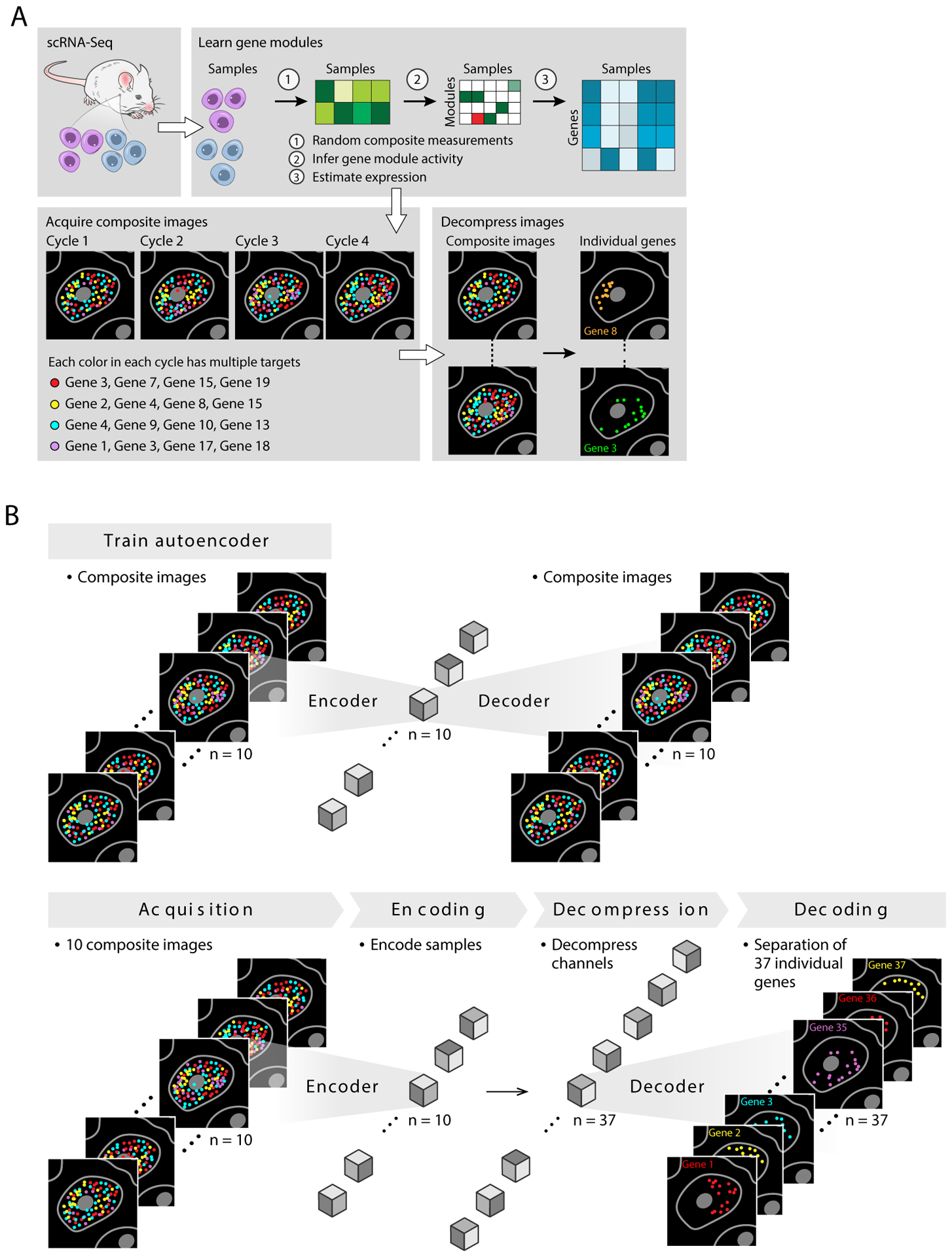
(a) Method overview. snRNA-Seq data (top left) is first analyzed (top right) to learn a dictionary of gene modules, simulate compressed sensing, and select measurement compositions to be used in CISI experiments (bottom left). In a CISI experiment, in each color in each round of imaging, probes for every gene in a given composite measurement are hybridized simultaneously. The process is repeated for different compositions over several cycles of stripping and hybridization (bottom left). Finally, composite images are then decompressed computationally (bottom right) to recover individual images for each gene. (b) Segmentation-free decompression. Top: An autoencoder is first trained on the composite images, with each composite measurement corresponding to one channel. Bottom: Once the autoencoder is trained, the composite images are encoded (“Encoding”), then decompressed to approximate the encoded representation for the unobserved image of each individual gene (“Decompression”), and the pre-trained decoder is used to recover individual images for each gene (“Decoding”).

In an alternative approach, we analyze the image without cell segmentation or explicit spot detection by using a convolutional autoencoder to infer individual gene abundances at each pixel in the image. Specifically, we use a convolutional autoencoder to compute a low-dimensional, encoded representation of each image, perform decompression in the encoded latent space, and then decode the encoded representation of each unobserved gene, outputting g individual images (Fig. 1b, Methods).

CISI offers two important advantages. Like combinatorial barcoding, CISI requires exponentially fewer rounds r of hybridization than linear barcoding (r_CISI = O(k ln(d)/c), r_{combinatorial} = ln(g)/c, and r_linear = g/c; we estimate that r_CISI and r_{combinatorial} will be comparable, with r_CISI/r_{combinatorial} typically between 1/3 and 3; Methods). But unlike combinatorial barcoding, CISI does not require spot-level resolution, and thus allows for low-magnification imaging and faster scanning over large volumes.

To demonstrate CISI, we first piloted it in the mouse primary motor cortex (MOp). We analyzed a set of 31,516 previously published single-nucleus RNA-Seq (snRNA-Seq) profiles from MOp (https://biccn.org/data). We chose to study g = 37 genes, consisting of 30 genes that are markers of either broader cell types (excitatory and inhibitory neurons, and various glial cells) or narrower subtypes (e.g., layer-specific inhibitory neurons) (Supplementary Table 1, Extended Data Figure 1), and 7 additional genes that were co-expressed with these markers.

We then learned a sparse modular representation of the expression of the 37 genes in the 27,491 cells where at least 1 of the 37 genes was detected. We used our method¹³ to identify a dictionary of d = 80 modules (Supplementary Table 2, Methods), such that the expression of each of the 37 genes can be represented with a linear combination of 3 or fewer modules with 94.3% correlation. This representation had high correlation with measured expression levels (88%), even in cells with greater than 5 of 37 genes expressed (Extended Data Figure 2a), and the 37 gene profiles for most cells were very accurately described (correlation >95%) by just 1 or 2 modules (Extended Data Figure 2b).

We then used the simulation procedure above to develop barcodes and composite measurements, optimizing the number of measurements (criterion (1); Extended Data Figure 3a), and the maximum number of compositions using each gene (criterion (2); Extended Data Figure 3b). Balancing the performance of the different designs and the estimated costs of probe synthesis, we selected the best performing set of 10 composite measurements, with each gene included in up to 3 compositions (Supplementary Table 3). Using these parameters, simulation refined performance from a median correlation of 76% with randomly chosen compositions, to 84% with the best performing selection, with compositions including between 6 and 13 genes.

We then experimentally tested the 10 selected compositions (Methods, Supplementary Table 4). For each of the 10 compositions, we imaged each gene individually, along with the pool of probes for the composition, together in the same tissue section. We merged the images acquired individually for each gene to create simulated composite images. Taking one composition as an example, the real and simulated composite images agreed well visually (Fig. 2a), and had 94.7% correlation between integrated intensity values in segmented cells (Fig. 2b). On average, across the 10 compositions the correlation was 90.1%.

Figure 2. CISI recovers accurate spatial expression patterns from composite experiments.

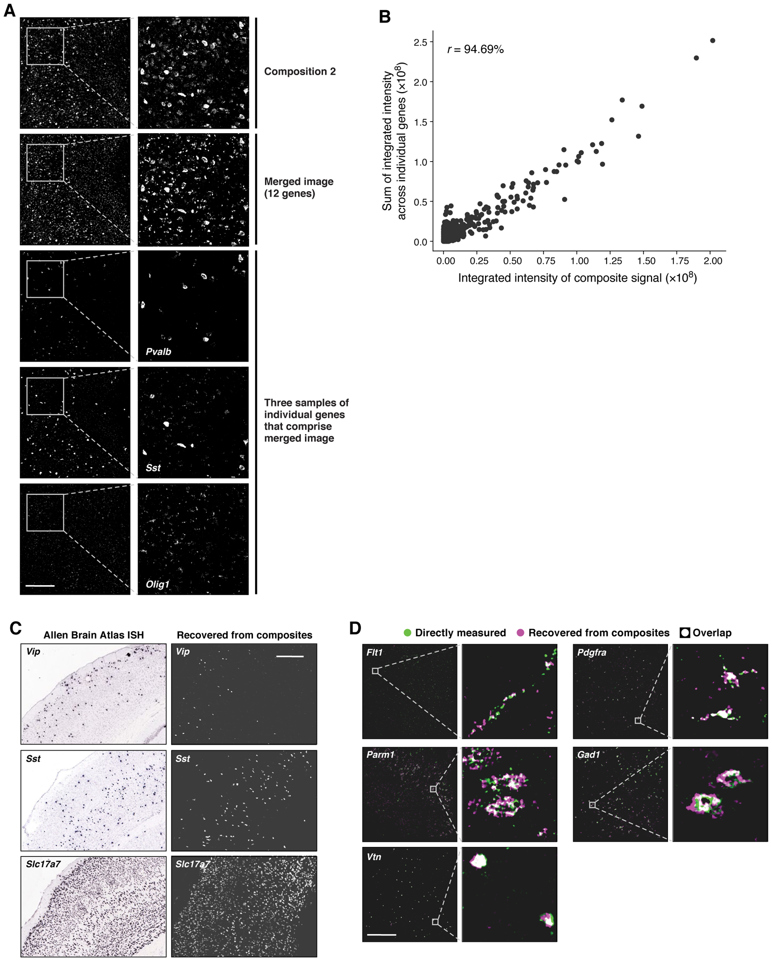
(a,b) Quantitative accuracy of the composite imaging. (a) A composite image of 12 genes (“Composition 2”) compared to a computational merge of 12 images for each individual gene (“Merged image”). 3 of the 12 individual gene images are shown for reference. Left: entire FOV; Right: zoomed in segment, as indicated. Scale bar: 500um. (b) The integrated signal intensity in each segmented cell (individual dots) in the composite image (x axis) and the merged image (y axis). Pearson’s r is noted in upper left corner. (c,d) Autoencoder based decompression successfully recovers accurate spatial patterns of individual genes. (c) Agreement with canonical expression patterns. Spatial RNA expression for Vip (top), a marker of a subtype of inhibitory neurons, which is expressed more frequently in layer 2/3; Sst (middle), a marker of another inhibitory neuron subtype, which is expressed more frequently in layer 5; and Slc17a7 (bottom), which is broadly expressed in excitatory neurons throughout MOp, by ISH (left; Allen Brain Atlas) and in the recovered images by the segmentation free algorithm (right). Scale bar: 500um. (d) Agreement with individual gene measurements on the same section. RNA images recovered by decompression with the segmentation free algorithm (magenta) and directly measured (green) in the same tissue section. White: images overlap exactly. Scale bar 500um. See also Extended Data Figure 4 for additional genes. Representative fields of view were selected to highlight expression of indicated genes, while quantification of overlap (correlation) was calculated using all cells in a given tissue section, or using randomly selected testing cells (where indicated).

Next, we generated a CISI imaging dataset, using our validated composite probe libraries, together with probes for individual genes (used only for later confirmation). In each tissue section comprising ~2,500–3,000 cells, we first imaged the 10 composite measurements over 3 1/3 rounds. Then, using the remaining two colors in the fourth round, and all three colors in a fifth round, we directly measured each of up to five individual genes, for subsequent validation. We repeated this in 8 tissue sections, picking different individual genes each time, such that in total we directly measured each of the 37 genes individually along with the compressed measurements (Supplementary Table 5).

We decompressed the experimental data with our segmentation-based and segmentation-free algorithms, and evaluated the accuracy of our results in several ways. First, the decompressed images for several genes corresponded well to their known distinct and readily identifiable spatial expression patterns in the Allen Brain Atlas (Fig. 2c). Second, the decompressed images agreed well with the direct measurements of each gene made in the same section (Fig. 2d and Extended Data Figure 4). The correlation between direct and decompressed measurements based on integrated signal intensity in segmented cells was high, either when using the segmentation-free autoencoding algorithm (83.6%) or when using decompression from segmented cells (88.4%). Both are in line with the simulations used to design our measurements, which predicted a correlation of 84%.

Notably, the segmentation-free autoencoder out-performs the segmentation-based algorithm for genes whose expression does not necessarily follow simple patterns (Extended Data Figure 5). While genes like Vtn have expression patterns easily captured by the filled polygons of segmented cells, others such as Flt1 and Parm1 are well-described by autoencoding, but not by segmentation (Fig. 2d, Extended Data Figure 5).

We analyzed cell-type composition of the autoencoding results, by segmenting cells post hoc (on decompressed images) and clustering the segmented cells based on the integrated intensity values across genes (Methods). Based on markers in each cluster, neurons comprised about half of all (successfully segmented) cells: 33.3% of cells in 9 excitatory clusters (vs. 44.5% of cells in snRNA-Seq), and 16.9% of cells in 6 inhibitory clusters (vs. 14.5%). In addition, we find 4 clusters of oligodendrocytes and oligodendrocyte precursor cells (16.8% vs. 8.9% in snRNA-Seq), 3 clusters of astrocytes (12.8% vs. 10.4%), 3 clusters of microglia (9.1% vs. 4.6%), 2 clusters of smooth muscle cells (6.5% vs. 1.9%) and 2 clusters of endothelial cells (4.4% vs. 15%). The under-representation of endothelial cells relative to snRNA-Seq may be due to challenges in segmenting them (Extended Data Figure 5).

The points of inaccurate recovery were relatively predictable and consistent between the two algorithms, with some false positives for several genes, but few false negatives (Extended Data Figure 6a). In each case of 8 genes with false positive results (Supplementary Table 6), the false positive signals co-occurred with a gene that had probes included in overlapping measurements. For instance, false positives for Hmha1 are found in cells that express Slc17a7 (Extended Data Figure 6c, left). Hmha1 is a member of two compositions, both of which also included Slc17a7, which is additionally included in a third composition. We developed a simple heuristic to address these errors, by adjusting one of the overlapping co-measured genes to zero (Methods). Applying this simple rule reduced false positives and improved the overall correlation from 83.6% to 88.6% with autoencoding, and from 88.4% to 91.6% with segmentation (Extended Data Figure 6a,b).

Using these adjusted values, decompressed measurements are substantially less sparse than snRNA-Seq (2.87 genes per cell on average in snRNA-Seq vs 5.96 or 6.49 using CISI with autoencoding or segmentation, respectively; Extended Data Figure 7a), while preserving the co-expression programs observed in snRNA-Seq. To compare co-expression patterns, we clustered cells in the (post hoc segmented) decompressed data (as above) and in snRNA-Seq (using only the 37 genes), finding 29 and 28 clusters, respectively, that were highly correlated and had identical sets of marker genes (Extended Data Figure 7b).

Encouraged by these results, we next generated a substantially larger dataset spanning 12 bisected coronal sections covering 180mm² and 476,276 analyzed cells (Fig. 3a). We substituted several genes for new genes that would allow us to evaluate performance for both cell type and cell state patterns. These included five immediate early genes (IEGs) that are markers of activity both broadly across cell types (Fos, Egr1) and within specific types (Egr4 in neurons, Klf4 in endothelial cells, Pou3f1 in OPCs)¹⁴. We also substituted six of our original genes with six cell type markers that are more commonly used in spatial transcriptomics studies (Supplementary Table 7; Fgfr3, Tyrobp, Fa2h, Prox1, Sv2c, and Calb1). With this modified panel of 37 genes, we used the Allen Institute Mouse Whole Cortex and Hippocampus SMART-seq dataset (RRID:SCR_019013) to learn gene modules and select measurement compositions. To avoid co-measured false positives challenges, we adjusted the criteria for selecting compositions to avoid overlaps (Methods), and increased the number of compositions to 11 and the maximum number of compositions per gene to 4 (Supplementary Table 8). In each tissue section we also individually probed several genes for direct validation (Supplementary Table 9). We imaged the tissue at 20X, and decompressed cells using the segmentation-based approach, which, in the current implementation, scales more effectively than the autoencoding approach. The initial decoded results were less accurate than in our pilot experiment (61.2% correlation with validation images vs 88.4% above), which we reasoned was partially due to differences between the training scRNA-Seq and our imaging data – especially expression profiles in the many brain regions that were imaged but not included in training.

Figure 3. CISI analysis of 12 bisected coronal brain sections efficiently recovers cell type, state, and diverse spatial patterns.

(A) Composite measurements and validation images were collected in 12 bisected coronal brain sections (greyscale showing DAPI), in total covering 180mm² and 476,276 cells. Composite measurements were decompressed to estimate the expression of 37 genes. Up to four genes were selected for validation in each tissue section. (B) RNA images are shown for two genes (Sv2c and Egr1) recovered by decompression with the segmentation-based algorithm (magenta) and directly measured (green) in the same tissue section. White: images overlap exactly. Correlation between recovered and validation images shown in parentheses. (C) Cells were clustered into 32 groups (legend) using the decompressed expression levels in all 12 tissue sections. Individual cells are colored based on their cluster label.

We thus developed a computational approach to optimize the module dictionary post hoc by using a portion of validation images collected in the new dataset to refine the modules and improve performance. We selected 60% of all cells at random in each tissue section, and optimized the modules to minimize reconstruction error in up to 4 out of 37 validated genes in each cell (Methods). Using this refined set of modules, we then evaluated performance on each of the validated genes in each section in the remaining 40% of cells, finding it substantially improved with an overall correlation of 81.3% (Supplementary Table 10).

The recovered expression levels correctly cluster genes into groups that correspond to known broad and specific cell subtypes (Extended Data Figure 8a,b), with generally good recovery across subtypes. We again find good reconstructions for genes with a broad spatial distribution, such as Slc17a7 or Egr1, and genes with highly-specific spatial expression, such as Sv2c and Tle4 (Fig. 3b and Supplementary Table 10). On average, IEGs were recovered at comparable accuracy to other genes, with the worst performance for Pou3f1, the most lowly-expressed IEG (Supplementary Table 10). Moreover, the conditional probability of IEG expression is concordant with scRNA and prior findings¹⁴: a subset of neurons, endothelial cells and OPCs express Egr4, Klf4 and Pou3f1, respectively, while Fos and Egr1 are more broadly distributed (Extended Data Figure 8c,d). This suggests that, with the chosen gene panel, CISI can be used to study cell types as well as cell states. Finally, cell clustering reveals that the recovered spatial patterns correctly capture well known cortical layers and subcortical spatial structures (Fig. 3c).

Several aspects of the results suggest potential limitations. First, some genes were less accurately recovered, with recovery accuracy 42% correlated with expression level and 44% correlated with the proportion of cells expressing a gene, such that rarely, lowly expressed genes were less accurately recovered (Extended Data Figure 9 and Supplementary Table 10). It may therefore be preferable to measure rarely, lowly expressed genes individually, rather than recover them from composites. This approach is in contrast, and perhaps complimentary, to combinatorial barcoding methods, which typically remove more highly abundant genes (that perform well in CISI) from combinatorial rounds, due to issues of spot crowding. Second, while existing methods that measure genes individually are more flexible, such that any pattern – or indeed, expression levels with no discernible pattern (spatial or otherwise) whatsoever – can be observed, CISI is constrained to a modular representation of co-expression patterns. However, this representation only applies at the level of individual cells, and thus does not assume any spatial patterning. Idiosyncratic expression, unique to one gene, for example due to transcriptional bursting or other inherent variability within single cells, may not be well-described by our method.

In conclusion, CISI addresses two key bottlenecks in imaging transcriptomics: increasing the number of genes studied per round of hybridization and decreasing the time needed to scan large tissue volumes per round. Compared with state-of-the-art linear multiplexing strategies⁹, in the results here we: reduced the number of rounds of imaging 2.5-fold (by assaying 37 genes with 11 compositions plus up to 4 validation images per section); reduced image acquisition time in the xy-plane 25-fold; and reduced acquisition time in the z-plane 8.6-fold. In total, this amounts to a 530-fold gain in efficiency. Much of the gain here is possible because CISI naturally adapts to low-magnification imaging. CISI aggregates signal locally (e.g., within a cell) and decompresses within this local space. If spots are well-separated they are computationally summed, while overlapping spots are physically summed (the pixels aggregate intensity). In contrast, at low-magnification, optical crowding critically undermines techniques using combinatorial barcodes (such as MERFISH or Seq-FISH).

Our results point towards the possibility of greatly increased throughput in imaging transcriptomics. CISI leverages algorithmic insights and biological structure to be more efficient in generating and interpreting data. Further applications using these principles¹⁵ could increase multiplexed protein detection with antibodies, make scRNA-seq more efficient by sequencing small pools of cells, or efficiently study genetic perturbations by leveraging common outcomes across experiments.

Methods

Mice

All mouse work was done with an adult C57B/L6 mouse according to IACUC procedures specified on protocol 0211-06-18, and we have complied with all relevant ethical regulations.

Analysis of single-nucleus RNA-Seq data

We selected 37 cell type/layer-specific markers by analyzing snRNA-seq data sets released by BICCN (U19 Huang generated by Regev lab; http://data.nemoarchive.org/biccn/grant/huang/macosko_regev/transcriptome/sncell/) for mouse primary motor cortex (M1 or MOp) and generated using the 10x single-cell 3′ protocol (V2). To align the reads, a custom reference was created by 10X Cell Ranger (v.2.0.1, 10X Genomics) using mouse genome and pre-mRNA annotation (Mus_musculus.GRCm38, release 84) according to the instructions provided on the 10X Genomics website (https://support.10xgenomics.com/single-cell-gene-expression/software/release-notes/build#mm10_1.2.0). The default parameters were used to align reads, perform UMI counting, filter high quality nuclei and generate gene by nucleus count matrices. In total, ~30,000 nuclei passed QC metrics including (i) the number of unique genes detected in each cell (>200) and (ii) the percentage of reads that map to the mitochondrial genome (<10%), and featured in the further downstream analyses using the Seurat package (version 2.2.1).

Compressed sensing simulations

We use compressed sensing to recover sparse signals from composite measurements. In the basic formulation, we seek to recover sparse gene module activities, $W\in {ℝ}^{d\times n}$, and estimate unobserved gene abundances, $UW=\widehat{X}\in {ℝ}^{g\times n}$ given observations $AUW=Y\in {ℝ}^{m\times n}$, a gene module dictionary $U\in {ℝ}^{g\times d}$, and measurement compositions $A\in {ℝ}^{m\times g}$, where there are m composite measurements of g genes in each of n cells, and the dictionary consists of d gene modules. This formulation is more tractable as an optimization problem than directly estimating gene abundance from low-dimensional observations, because in the modular representation W is sparse, with few non-zero parameters. While the small amount of data we collect, Y, is insufficient data to directly estimate all of the parameters of X, it is sufficient to infer these few parameters of W.

Using the snRNA-Seq data above, and the 37 selected genes, we evaluated different composite designs by simulating composite measurements and recovering individual expression levels by sparse optimization (as previously described¹³; see also https://github.com/cleary-lab/CISI). Briefly, we first randomly selected training, validation and testing subsets, using 60%, 20%, and 20% of all cells for each respective group. In the training set, we calculated a dictionary, $U\in {ℝ}^{g\times d}$, with d = 80 modules of g = 37 genes (and default SMAF parameters found on https://github.com/cleary-lab/CISI). A given simulation trial with m measurements consists of (i) randomly assigning genes to compositions, A; (ii) simulating noisy composite measurements in validation data, $Y=A\left(X+ϵ\right)$ (with $ϵ\in {ℝ}^{m\times n}$ drawn i.i.d. from a normal distribution with variance adjusted to achieve a signal-to-noise ratio of 5); (iii) decoding sparse module activity levels, $mi{n}_W\Vert W{\Vert }_1;s.t.\frac{\Vert Y-AUW\Vert }{\Vert Y\Vert }<\lambda$; (iv) estimating individual expression levels, $\widehat{X}=UW$; and (v) calculating the correlation between the original and estimated levels, $\mathit{\text{corr}}=\mathit{\text{Pearson}}\left(X,\widehat{X}\right)$. When evaluating different measurement designs in step (i), we varied the total number of measurements (from 8 to 12), and the maximum number of measurements in which each gene appeared (either 2, 3, or 4). Each gene was then randomly assigned to a randomly chosen number of measurements (up to the maximum). Final assignments resulting in either two or more genes being perfectly co-assigned or in large measurement imbalance (any gene appearing more than 4 times more frequently than any other gene) were excluded. We then iterated steps (i)-(v) 2,000 times, selected the 50 composition matrices resulting in the top correlations, and evaluated (steps (ii)-(v)) in testing data. The correlations in testing data were then used to compare different numbers of measurements, and maximum assignments per gene (Extended Data Figure 3).

Selection of the final library

For the initial study, based on the comparisons in Extended Data Figure 3, and considering the number of probes that would need to be synthesized in each scenario, we selected the composition with the highest performance in testing data among those with 10 measurements and a maximum of 3 assignments per gene. Each of the 10 compositions was assigned to one of three colors, to be imaged during 3 1/3 rounds (Supplementary Table 2).

For the larger study with 12 coronal sections we simulated compositions with 11 genes and 4 assignments per gene to reduce the number of exact overlaps (e.g., where one gene is assigned to 2 compositions, and those 2 compositions match 2 of 3 assignments for a second gene). From among the top 50 performing compositions in simulation with no exact overlaps, we selected the composition which had the fewest number of large overlaps, where a gene has a large overlap if more than 66.7% of its assignments matched the assignments for at least one other gene.

Probe design and validation

For each target mRNA, HCRv3.0 DNA probe sets of ~20 probe pairs each were ordered from Molecular Technologies, or designed in-house and ordered from IDT. All HCR v3.0 reagents are available from Molecular Instruments, Inc. (molecularinstruments.com). Target binding site sequences can be found in Supplementary Table 4.

Tissue preparation and brain extraction

An adult C57B/L6 mouse was perfused with ice-cold PBS (10010023, ThermoFisher Scientific) prior to dissection of the brain. The brain was then extracted and flash frozen in liquid nitrogen. After OCT embedding, the brain was sectioned directly into an APTES coated 24-well glass bottom plate (82050–898, VWR). For coating, plates were coated with a 1:50 solution of APTES (440140, Sigma) in 100% Ethanol (V1016, DeconLabs) for 5 minutes followed by 3x washes with 100% ethanol before drying. Tissues were fixed in 10% Formalin (100503–120, VWR) for 15 minutes and washed with PBS before overnight permeabilization with 70% ethanol. Tissues were re-hydrated with PBS prior to hybridization. In the larger study, we added a tissue clearing step: re-hydrated sections were cleared briefly with two five-minute washes of 4% SDS (BM-230, Boston BioProducts) prior to hybridization.

In situ hybridization

In situ HCR version 3.0 with split-initiator probe sets was performed using the protocol detailed in¹⁰ with some slight adaptations. Probe sets for each individual target mRNA were diluted to the concentration specified in the protocol and organized into composite channels. A composite channel is comprised of a mix of probe sets for approximately 10 different target mRNAs, each with the same initiator. In total, 10 composite channels were created. Three composite channels can be hybridized per round of imaging. Thus, for the first round of hybridization, probe sets for three composite channels with distinct initiator sequences were added at once to each tissue.

Probes were hybridized for approximately 8 hours in hybridization buffer and then tissues were washed 3 times with 30% probe wash buffer for 10 mins each at 37C and 1 wash of 5X SSCT for 10 mins at room temperature (buffer compositions available from Molecular Instruments). Snap-cooled hairpins were added at a 1:200 diluted concentration and amplification was allowed to proceed for 8 hours. Excess hairpins were then washed off with 3 washes of 5X SSCT (15557044, ThermoFisher Scientific), for 5 minutes each. Tissues were stained with DAPI (1:5,000 TCA2412–5MG, VWR) immediately prior to imaging. After imaging, probes were stripped from tissues using 80% formamide at 37°C for 60 minutes. This entire process (hybridization, amplification, imaging, stripping) was repeated for up to five rounds of imaging (see Supplementary Table 5 for composites and individual targets imaged in each round). All DNA HCR amplifiers (hairpins), hybridization buffers, wash buffers, and amplification buffers were ordered from Molecular Technologies. All HCR v3.0 reagents are now only available from Molecular Instruments, Inc. (molecularinstruments.com).

Imaging

Imaging was performed on a spinning disk confocal microscope (Yokogawa W1 on Nikon Eclipse Ti) equipped with a Nikon CFI APO LWD 40x/1.15 water immersion objective or a 20× 0.8 plan apo lambda objective operating NIS-elements AR software with Andor Zyla 4.2 sCMOS detector. DAPI fluorophores were excited with a 405nm laser, Alexa 488 HCR amplifiers were excited with a 488nm laser with 525/36 emission filter (Semrock, 77074803), Alexa 546 HCR amplifiers were excited with a 561nm laser with a 582/15 emission filter (Semrock, FF01–582/15–25), and Alexa 647 HCR amplifiers were excited with a 640nm laser with a 705/72 emission filter (Semrock, 77074329).

Image processing

Before downstream analysis, we ran a series of image processing steps to normalize, stitch, align, and segment the images in each color, field of view, round, and tissue. In the pilot study, we first took a maximum projection across the z-axis, and then used the DAPI channel to stitch the fields of view within each round of imaging (using ImageJ software¹⁶). We applied the stitching coordinates from the DAPI channel to each of the other channels. We then smoothed the image for each channel using a median filter (with a width of 8 pixels). (If spot-level resolution is needed, this step may not be advised. Since we do not need this resolution, we use this step to make autoencoder reconstruction an easier task.) From each smoothed image, we aligned and subtracted background signal, obtained by imaging after stripping the final round of fluorescent probes. We then adjusted brightness and contrast by rescaling according to upper and lower thresholds determined using auto-adjust in ImageJ. The same rescaling parameters for each channel (determined from the maximum upper threshold and minimum lower threshold) were applied to all tissues and rounds. After rescaling, we applied a flat field correction to each field of view, by normalizing (dividing) each pixel by the median smoothed pixel intensity across all images (with smoothing by a Gaussian filter with a width 1/8 of the image dimension). Each round of the flat field-corrected images in a given tissue was then aligned using ImageJ. These images were used in the remainder of downstream analysis.

In the larger dataset we used a modified procedure (detailed here: https://github.com/cleary-lab/CISI). Briefly, raw images for each section and round were first stitched using the BigStitcher plugin for ImageJ¹⁷. The Starfish pipeline¹⁸ was used to remove background and call spots (allowing for the detection of large, closely-spaced “spots” to account for low-magnification imaging) in each stitched image. The output was used to create masks and produce filtered images with background removed. Filtered images were aligned across rounds within each section. In some sections, either the stitching or alignment failed in a portion of the section in one or more rounds. These regions were masked and excluded from downstream analysis by comparing stitched and aligned DAPI images from each round, and manually drawing masks around the affected regions.

For segmentation, we used CellProfiler¹⁹, and calculated one image mask per nucleus in each tissue using DAPI in the first round. Each mask was then expanded by up to 10 pixels (without overlapping a neighboring cell). Comparisons and decompression with segmented cells were done using the integrated image intensity in each expanded nucleus mask.

Decompression of composite signals

We developed two methods to decompress composite signal intensities into signals for individual genes.

The first method, which we used primarily as a point of reference for validation statistics, is based on cell segmentation. Given the intensities of each composite measurement in each segmented cell, $Y\in {ℝ}^{m\times n}$, we solved a sparse optimization problem to decode sparse module activity levels, $mi{n}_{W\in {ℝ}^{d\times n}}\Vert W{\Vert }_1;s.t.\frac{\Vert Y-AUW\Vert }{\Vert Y\Vert }<\lambda$, before estimating individual expression levels, $\widehat{X}=UW$, with the same method as in our simulations (above).

The second method we developed decompresses entire images using a convolutional autoencoder. In this approach, for a given set of 10-channel composite images, we first train a model to identify a reduced (encoded) representation of each image, which can then be decoded to recapitulate the original. During this training, we optimize the following loss function:

$${\Vert \text{log}\left(Y+\epsilon \right)-\text{log}\left(\widehat{Y}+\epsilon \right)\Vert }_1+{\lambda }_{\mathit{\text{pixel}}}{\mathcal{L}}_{\mathit{\text{pixel}}}+{\lambda }_{\mathit{\text{TV}}}{\mathcal{L}}_{\mathit{\text{TV}}},$$

where Y is the original image, $\widehat{Y}$ is the decoded image, ${\mathcal{L}}_{\mathit{\text{pixel}}}$ is a loss on pixel density, ${\mathcal{L}}_{\mathit{\text{TV}}}$ is the total variation of $\widehat{Y}$ , λ_pixel and λ_TV are hyperparameters, and ε is a small constant. ${\mathcal{L}}_{\mathit{\text{pixel}}}$ is calculated as the Poisson log-likelihood of the pixel density, which is computed as the Shannon Diversity across pixels, divided by the number of pixels, with prior density set by a parameter δ_pixels. Convolutions in each layer of the network are computed across filters (or kernels), but not across the 10 composite channels. Hence, each of the 10 channels remains separated from the other channels throughout each layer of the network. However, only one set of convolutional weights is learned; these are shared across all channels. The number of parameters in the model is, thus, relatively small, and the autoencoder trained quickly on our data. As discussed below, hyperparameters, including the number of encoding and decoding layers, the number and size of filters, and pooling sizes are chosen by hyperparameter tuning on a small set of validation images.

Using the trained autoencoder, we decompress composite images as follows. First, we encode each 10-channel image to a reduced representation, $\tilde{Y}\in {ℝ}^{10\times \tilde{w}\times \tilde{h}\times f}$, where $\tilde{w}$ and $\tilde{h}$ are the reduced width and height (after pooling at each encoding layer), and f is the number of convolutional filters. We then solve for sparse module activities, $\tilde{W}\in {ℝ}^{d\times \tilde{w}\times \tilde{h}\times f}$, where d is the number of modules in the dictionary (here, 80), and then estimate the encoded representation of each individual (unobserved) gene, $\tilde{X}\in {ℝ}^{37\times \tilde{w}\times \tilde{h}\times f}$. These representations are then run through the pre-trained decoder to produce an image for each gene, $\widehat{X}\in {ℝ}^{37\times w\times h}$.

Our loss function has components at both the encoding and decoding layers:

$$\mathcal{L}={\Vert \tilde{Y}-AU\tilde{W}\Vert }_2^2+{\Vert \text{log}\left(Y+\epsilon \right)-\text{log}\left(A\widehat{X}+\epsilon \right)\Vert }_1+{\lambda }_{\mathit{\text{pixel}}}{\mathcal{L}}_{\mathit{\text{pixel}}}+{\lambda }_{\mathit{\text{TV}}}{\mathcal{L}}_{\mathit{\text{TV}}}+{\lambda }_W{\mathcal{L}}_W,$$

where ${\mathcal{L}}_W$ is a loss on the density of $\tilde{W}$, calculated as the Poisson log-likelihood of the Shannon diversity, with prior density set by parameter δ_W. We implemented our model in tensorflow, using the Adam optimizer.

Hyperparameters and model architectures were chosen by hyperparameter tuning on a small set of validation images. The validation images consist of 4 of 36 patches from each of 3 images (i.e., from 3 tissue sections, each with 36 patches), for a total of 12 patches (equivalent in size to 1/3 of one image). Each patch includes signal from the 10 composite measurements, along with up to 5 directly measured genes. In each validation trial, we select hyperparameters, train the autoencoder on the composite data, decompress all genes, and then calculate the trial score as the correlation between the subset of directly measured and recovered genes (this is done in post hoc segmented cells, when using the autoencoder). We selected the hyperparameters from the best performing trial, and used these to run our analysis on the full dataset. More details can be found at https://github.com/cleary-lab/CISI.

We applied a heuristic correction to co-measured genes. We first identified 104 pairs of co-measured genes (i.e., that co-occur in more than one composition) that were not correlated (<10%) in snRNA-Seq. For each pair, we set the expression of one of the two genes to zero whenever they were co-expressed in recovered images. To select which gene to adjust, we calculate the correlation between the 10 composite measurements in a cell, and the pattern of measurements for each of the two genes (e.g., the binary vector indicating which measurements included the gene), and then adjust to zero the gene with the lower correlation.

Optimization of the module dictionary using validation images

For the segmentation-based approach, we developed a method to update the module dictionary, U, using the validation images collected in each tissue section. We initialized the dictionary with the dictionary found from scRNA-Seq training data. In each iteration of this method, we first use the current dictionary to decode sparse module activity levels, W, as described above (Decompression of composite signals). We then update U via gradient descent (as implemented by the AdamOptimizer function in TensorFlow) on the following loss function:

$$\mathit{\text{loss}}=\sum _{j=1}^n\sum _{i\in V_j}\frac{{\left(x_{i,j}-{\widehat{x}}_{i,j}\right)}^2}{s_i}+{\lambda }_{\mathit{\text{corr}}}\mathit{\text{los}}{s}_{\mathit{\text{corr}}}+{\lambda }_{\mathit{\text{cond}}}\mathit{\text{los}}{s}_{\mathit{\text{cond}}}$$

where V_j is the set of up to 4 genes validated in each section and s_i is the scale of each gene (defined as the 75^th percentile of nonzero expression). The first term penalizes reconstruction error, while the second and third penalize differences from scRNA-Seq training data in correlation structure and conditional probabilities, respectively. Specifically,

$$\mathit{\text{los}}{s}_{\mathit{\text{corr}}}=\sum _{j=1}^n\sum _{k=j+1}^n{e}^{{\left(c_{j,k}-{\widehat{c}}_{j,k}\right)}^2}-1$$

and

$$\mathit{\text{los}}{s}_{\mathit{\text{cond}}}=\sum _{j=1}^n\sum _{k\ne j}^n{e}^{{\left(p_{j,k}-{\widehat{p}}_{j,k}\right)}^2}-1$$

where c_j,k is the correlation between genes j and k in scRNA-Seq, ${\widehat{c}}_{j,k}$ is the correlation between genes j and k in decompressed results, and p_j,k and ${\widehat{p}}_{j,k}$ are the probabilities of gene k expression conditioned on gene j in scRNA-Seq and CISI respectively. The exponential form of these penalties was chosen so that the loss would be similar to the squared deviation for small differences, while scaling much faster for large differences. The method was run for 25 epochs with 5,000 cells per iteration batch.

When updating the dictionary in this way we first partitioned the cells into training (60%) and testing (40%). To find optimal hyperparameters (λ_corr and λ_cond) we perform a grid search over 100 pairs of parameters. For each pair, we update the dictionary using training cells, and then use this dictionary to decompress composite measurements in test cells. We select the pair of hyperparameters for which performance (here, average gene-wise reconstruction correlation) rapidly decays when increasing either parameter individually (λ_corr = 1.0 and λ_cond = 2.15).

Plotting decompressed images

The decompressed results for each gene vary in their relative signal intensities (as do direct measurements for each gene). When plotting merged validation images (as in fig. 2d and Extended Data Figure 4), we normalize the signal for each gene to automatically adjust contrast and brightness. The specific parameters of this normalization can be found in the code demo of our online repository (https://github.com/cleary-lab/CISI/blob/master/getting_started/plot_decompressed_images.py). The signal plotted for direct measurements have been pre-processed according to the methods described above.

Comparison of CISI and combinatorial barcoding

We can approximate the number of imaging rounds in CISI, r_CISI, relative to that in combinatorial barcoding methods, r_{combinatorial}, defined as r_CISI/r_{combinatorial}, based on our results here, using simulation to extrapolate to larger scales, and by comparing with existing combinatorial methods. Here, we used 3 and 2/3 rounds to measure 37 genes; the same could be achieved using 3-color combinatorial barcoding without error correction. More commonly, 4 or 5 rounds would be used to measure 37 genes and allow for error correction. At larger scales, simulations in our earlier work¹³ suggest that ~100 composite measurements would suffice to approximate the expression of 10,000 genes. This could be done in 33 and a 1/3 rounds of CISI. To date, the only combinatorial method to scale to this level did so with 80 rounds of imaging¹². We therefore very roughly approximate that the required rounds of imaging with either approach will be comparable, and that r_CISI/r_{combinatorial} will be in the range 1/3 to 3, allowing for improvements in combinatorial methods and the possibility of needing more rounds than anticipated with CISI.

Data availability

We used publicly-available snRNA-Seq data sets released by BICCN (U19 Huang generated by Regev lab; http://data.nemoarchive.org/biccn/grant/huang/macosko_regev/transcriptome/sncell/), and full-length scRNA-Seq (the Allen Institute Mouse Whole Cortex and Hippocampus SMART-seq (RRID:SCR_019013)). Raw image data from the large validation study are available for download at the Brain Imaging Library: https://download.brainimagelibrary.org/49/77/49777378713bb584/.

Code availability

An online repository of code used in this study can be found at https://github.com/cleary-lab/CISI.

Extended Data

Extended Data Fig. 1. Marker gene expression in snRNA-seq clusters.

For each of 37 genes, shown is the distribution of expression (individual violin plots; y-axis) in each of 23 snRNA-Seq clusters (x axis). Marker genes for similar cell types are grouped together with the cell type labeled on top.

Extended Data Fig. 2. Analysis of modular factorization based on gene and module diversity.

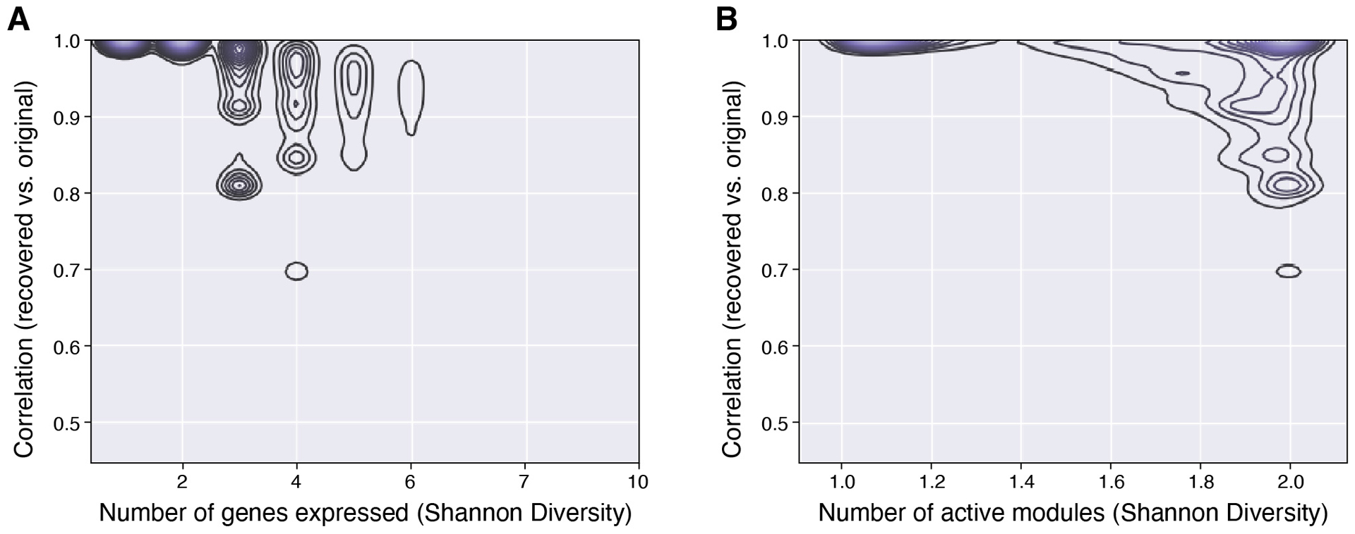
Pearson correlation (y-axis) between the original expression levels of 37 genes in each cell and those approximated in those cells by Sparse Module Activity Factorization (SMAF). Contour plots depict the density of cells at each level of correlation with either a given number of genes expressed (a; x-axis) or a given number of gene modules by SMAF decomposition (b; x-axis).

Extended Data Fig. 3. Evaluation of performance of simulated compositions.

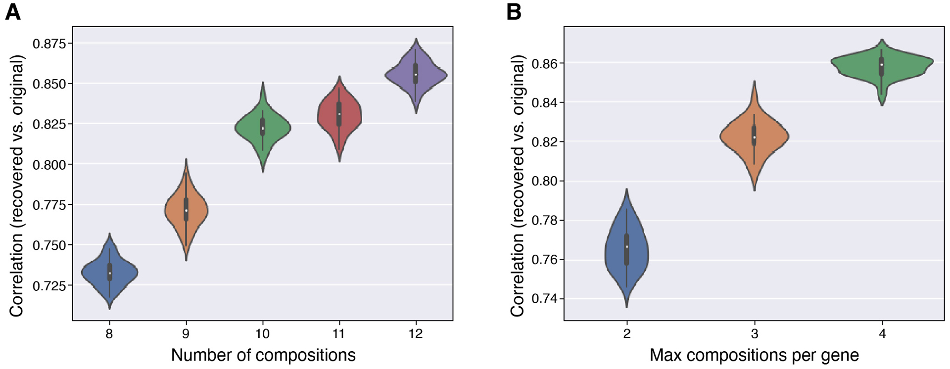
Distribution of Pearson correlation between the original and recovered expression levels of 37 genes in each cell (y axis) across simulation trials for different numbers of composite measurements (a), or for different measurement densities, set by the maximum number of measurements in which each gene was included (b). In (a) the maximum compositions per gene is 3, and in (b) the number of compositions is 10. Mini boxplots depict median (center dots), inner quartiles (upper and lower bounds of box for 25^th and 75^th percentile), and 1.5x quartile range (minima and maxima of whiskers).

Extended Data Fig. 4. Autoencoder based decompression successfully recovers accurate spatial patterns of individual genes compared to direct measurement on the same section.

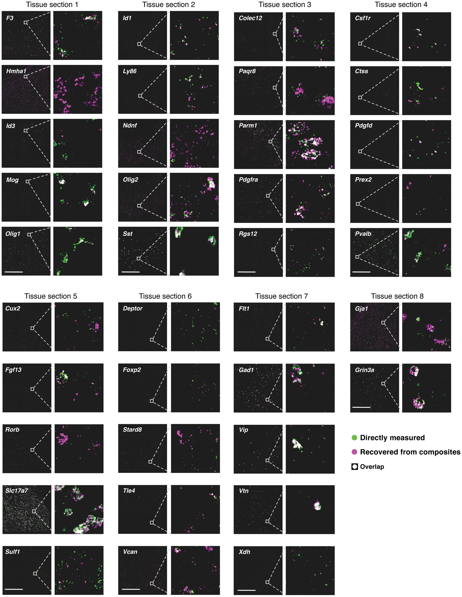
RNA images recovered by decompression with the segmentation free algorithm (magenta) and directly measured (green) in the same tissue section. White: images overlap exactly. Genes are grouped based on the section in which their direct measurements were made. Insets for all genes in a section show the same region, or an adjacent region if no cells for a given gene were present. Scale bar: 500um. Representative fields of view in each tissue section were chosen such that every gene validated in a tissue section could be visualized in the same region, while quantification of overlap (correlation) was calculated using all cells in a given tissue section, or using randomly selected testing cells (where indicated).

Extended Data Fig. 5. Comparison of autoencoding and segmentation-based decompression.

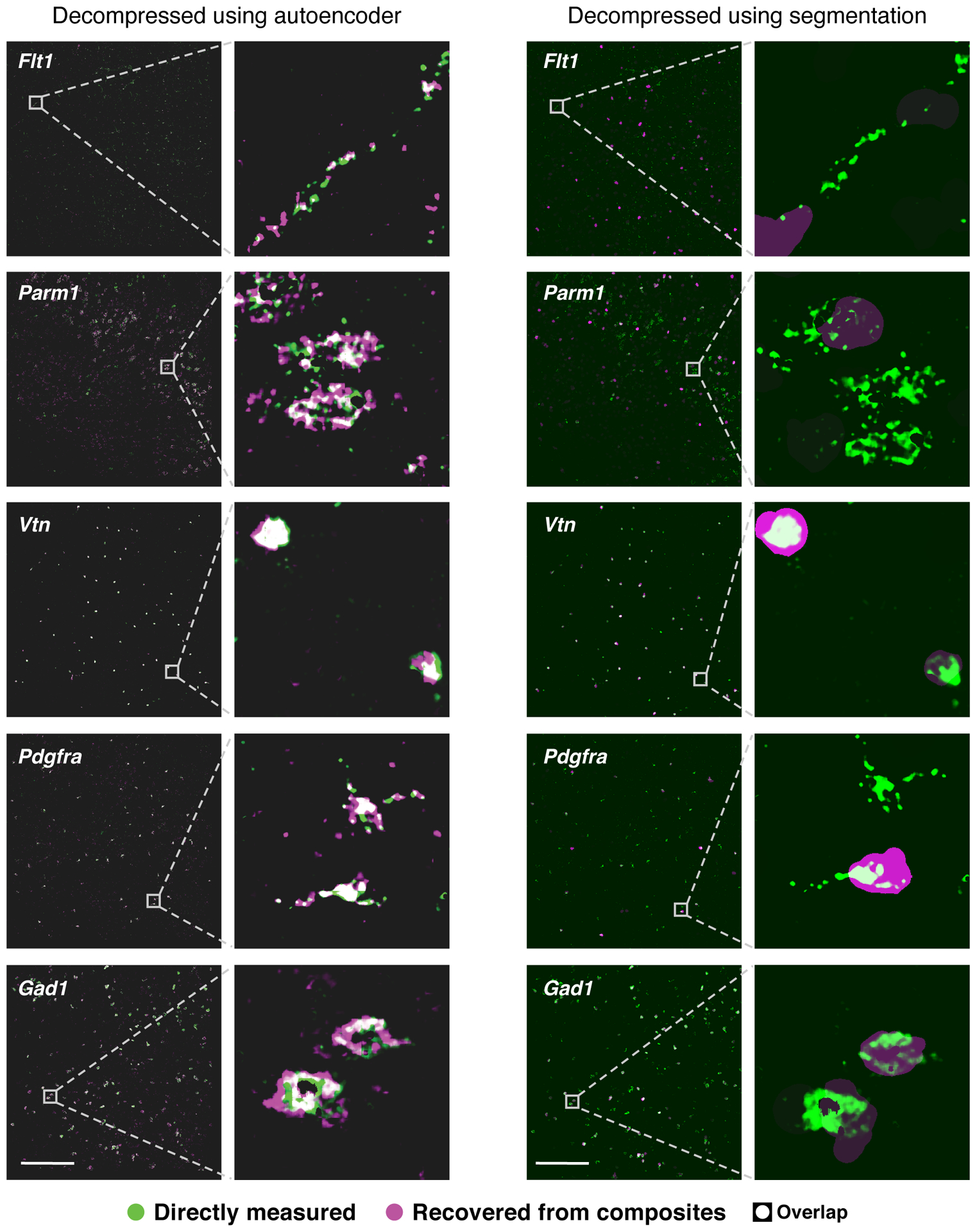
Individual gene images recovered (magenta) using the autoencoding algorithm (left) or the segmentation based algorithm (right) are overlaid with direct measurement (green) of the genes in the same tissue sections (white: direct overlap). For segmentation-based decompression, the decompressed signal for each gene is projected uniformly over each segmentation mask. Scale bar: 500um. Representative fields of view were selected to highlight expression of indicated genes, while quantification of overlap (correlation) was calculated using all cells in a given tissue section, or using randomly selected testing cells (where indicated).

Extended Data Fig. 6. Evaluation of recovered signals before and after co-measurement adjustment.

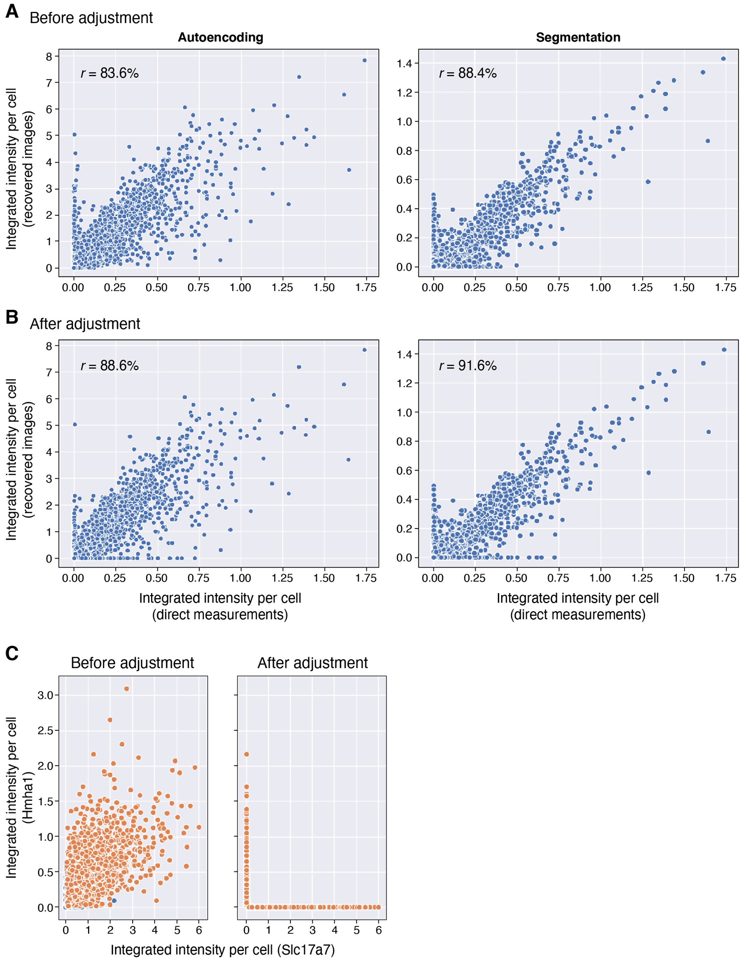
(a,b) Adjustment improves recovered signals. Integrated signal intensity for each gene in each cell (individual dots) from direct measurements (x axis) and from estimates recovered by the autoencoder decompressed images (y axis) either before (a) and after (b) co-measurement correction. (c) Example correction. Segmented cell intensities before (left) and after (right) correction for two co-measured genes (Hmha1 and Slc17a7) that were not correlated in snRNA-Seq.

Extended Data Fig. 7. Evaluation based on genes per cell and cell clusters.

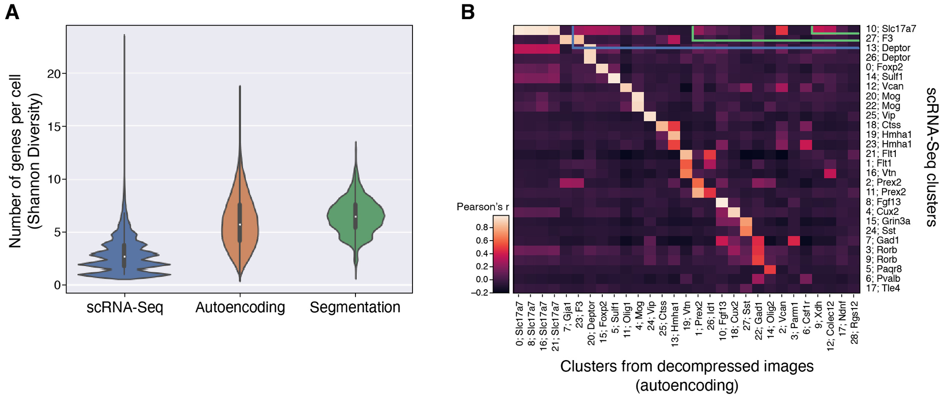
(a) Distribution of expression diversity (effective number of genes expressed per cell out of 37 total; y axis) in snRNA-Seq, or based on recovered expression levels using autoencoding or segmentation-based decompression (x axis). Mini boxplots depict median (center dots), inner quartiles (upper and lower bounds of box for 25^th and 75^th percentile), and 1.5x quartile range (minima and maxima of whiskers). (b) Correspondence (Pearson’s correlation of mean gene expression; color bar) between cell clusters from snRNA-Seq (rows) and those found from post hoc segmentation of images recovered using the autoencoding algorithm (columns). One marker gene for each cluster is indicated.

Extended Data Fig. 8. CISI recapitulates clusters and conditional probabilities from scRNA-Seq.

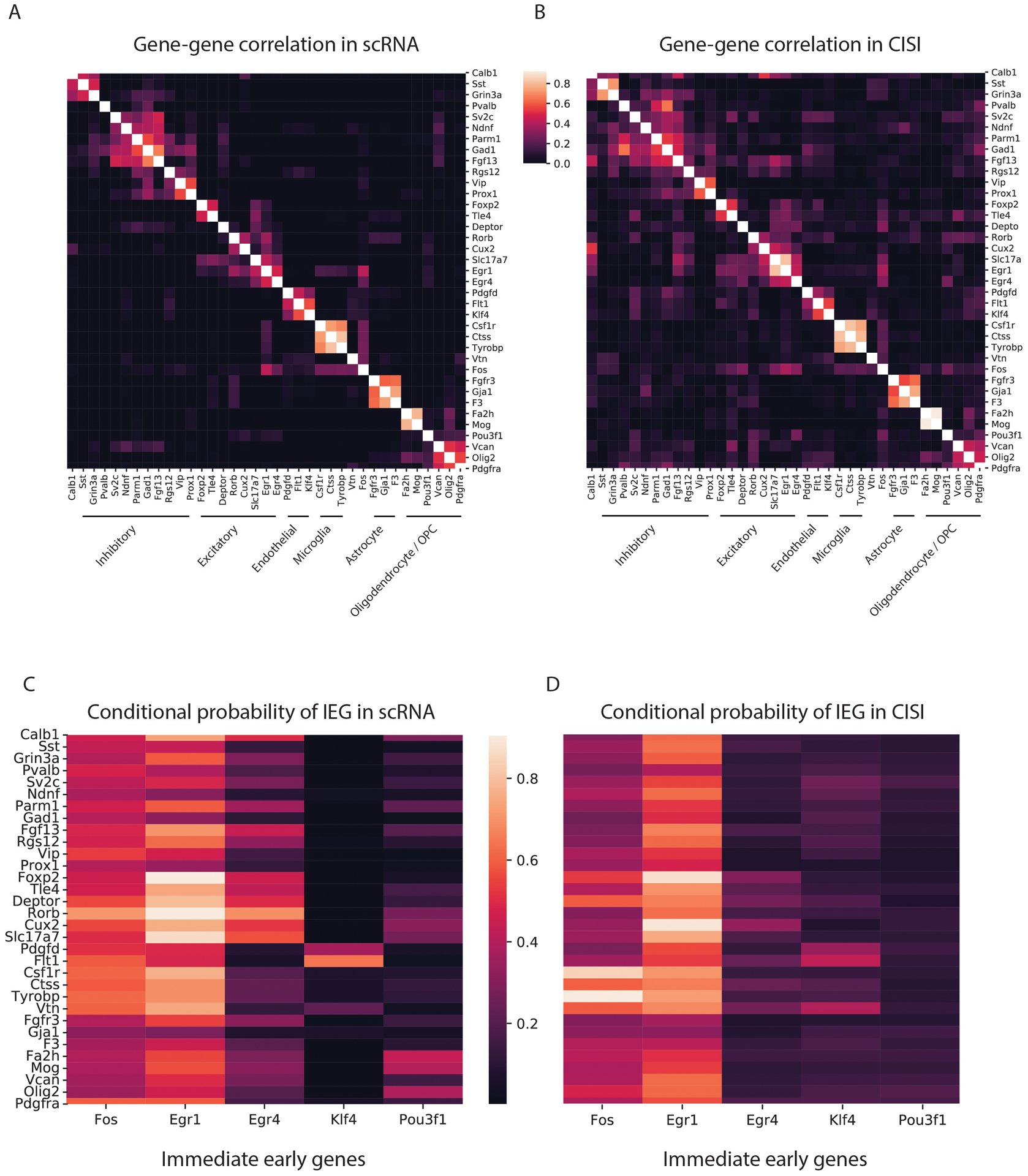
(a,b) Consistent identification of cell type specific gene programs in scRNA-Seq and CISI. The correlation coefficient (colorbar) between pairs of genes (row and column labels) in scRNA-Seq (a) and decompressed CISI measurements (b). Rows and columns are clustered. Gene clusters of cell type specific markers are labeled by the respective cell type. (c,d) Consistent cell type expression patterns for IEGs in scRNA-Seq is CISI. Conditional probability (colorbars) of IEGs (columns) in cells that express a given gene (rows) in scRNA-Seq (c) and decompressed CISI (d) data.

Extended Data Fig. 9. Gene-level correlation with validation measurements.

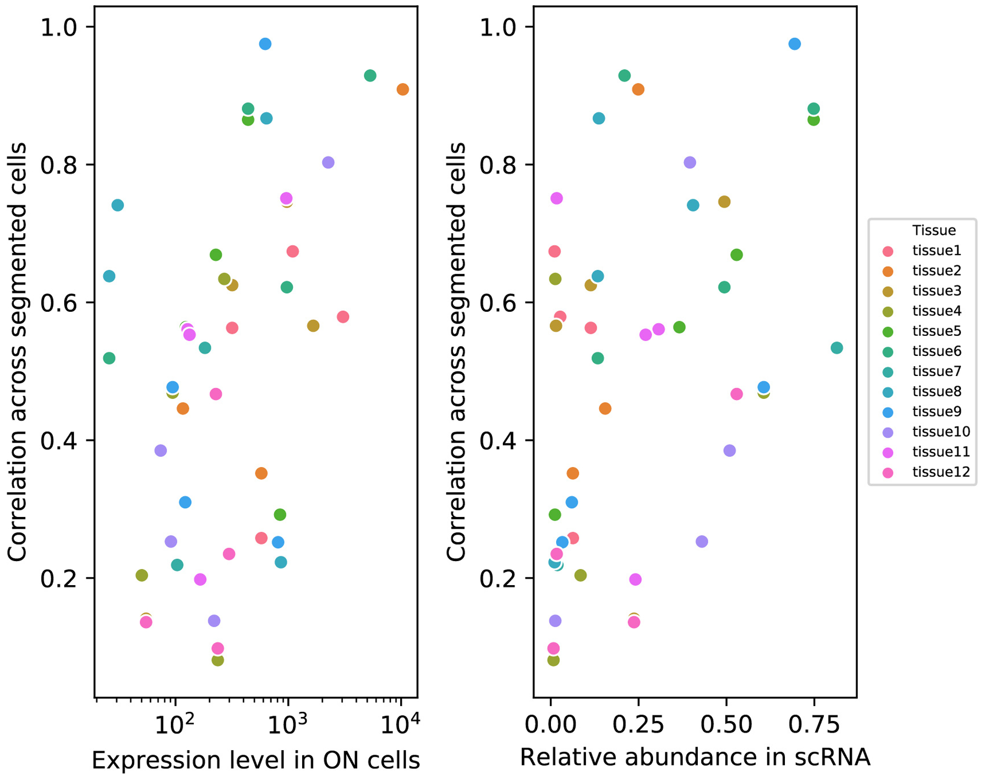
For each gene (individual dots) validated in each tissue (colors) the correlation across all segmented cells (y-axis) between values recovered by CISI and directly measured values is plotted vs the average expression level (TPM) in cells expressing the gene in scRNA-Seq (x-axis, left), or the percentage of cells expressing the gene (x-axis, right). Individual data points labeled by gene are provided in Supplementary Table 10.

References:

- 1.Angelo M et al. Multiplexed ion beam imaging of human breast tumors. Nat. Med 20, 436–42 (2014). [DOI] [PMC free article] [PubMed] [Google Scholar]
- 2.Keren L et al. A Structured Tumor-Immune Microenvironment in Triple Negative Breast Cancer Revealed by Multiplexed Ion Beam Imaging. Cell 174, 1373–1387.e19 (2018). [DOI] [PMC free article] [PubMed] [Google Scholar]
- 3.Goltsev Y et al. Deep Profiling of Mouse Splenic Architecture with CODEX Multiplexed Imaging. Cell 203166 (2018). doi: 10.1016/j.cell.2018.07.010 [DOI] [PMC free article] [PubMed] [Google Scholar]
- 4.Chen KH, Boettiger AN, Moffitt JR, Wang S & Zhuang X Spatially resolved, highly multiplexed RNA profiling in single cells. Science (80-.). 348, aaa6090–aaa6090 (2015). [DOI] [PMC free article] [PubMed] [Google Scholar]
- 5.Shah S, Lubeck E, Zhou W & Cai L In Situ Transcription Profiling of Single Cells Reveals Spatial Organization of Cells in the Mouse Hippocampus. Neuron (2016). doi: 10.1016/j.neuron.2016.10.001 [DOI] [PMC free article] [PubMed] [Google Scholar]
- 6.Shah S, Lubeck E, Zhou W & Cai L seqFISH Accurately Detects Transcripts in Single Cells and Reveals Robust Spatial Organization in the Hippocampus. Neuron (2017). doi: 10.1016/j.neuron.2017.05.008 [DOI] [PubMed] [Google Scholar]
- 7.Wang X et al. Three-dimensional intact-tissue sequencing of single-cell transcriptional states. Science (80-.). (2018). doi: 10.1126/science.aat5691 [DOI] [PMC free article] [PubMed] [Google Scholar]
- 8.Wang G, Moffitt JR & Zhuang X Multiplexed imaging of high-density libraries of RNAs with MERFISH and expansion microscopy. Sci. Rep (2018). doi: 10.1038/s41598-018-22297-7 [DOI] [PMC free article] [PubMed] [Google Scholar]
- 9.Codeluppi S et al. Spatial organization of the somatosensory cortex revealed by osmFISH. Nat. Methods 15, 932–935 (2018). [DOI] [PubMed] [Google Scholar]
- 10.Choi HMT et al. Third-generation in situ hybridization chain reaction: multiplexed, quantitative, sensitive, versatile, robust. Development 145, dev165753 (2018). [DOI] [PMC free article] [PubMed] [Google Scholar]
- 11.Raj A, van den Bogaard P, Rifkin SA, van Oudenaarden A & Tyagi S Imaging individual mRNA molecules using multiple singly labeled probes. Nat. Methods (2008). doi: 10.1038/nmeth.1253 [DOI] [PMC free article] [PubMed] [Google Scholar]
- 12.Eng CHL et al. Transcriptome-scale super-resolved imaging in tissues by RNA seqFISH+. Nature (2019). doi: 10.1038/s41586-019-1049-y [DOI] [PMC free article] [PubMed] [Google Scholar]
- 13.Cleary B, Cong L, Cheung A, Lander ES & Regev A Efficient Generation of Transcriptomic Profiles by Random Composite Measurements. Cell 171, 1424–1436.e18 (2017). [DOI] [PMC free article] [PubMed] [Google Scholar]
- 14.Hrvatin S et al. Single-cell analysis of experience-dependent transcriptomic states in the mouse visual cortex. Nat. Neurosci (2018). doi: 10.1038/s41593-017-0029-5 [DOI] [PMC free article] [PubMed] [Google Scholar]
- 15.Cleary B & Regev A The necessity and power of random, under-sampled experiments in biology. arXiv Prepr. arXiv2012.12961 (2020). [Google Scholar]
- 16.Abràmoff MD, Magalhães PJ & Ram SJ Image processing with imageJ. Biophotonics International (2004). [Google Scholar]
- 17.Hörl D et al. BigStitcher: reconstructing high-resolution image datasets of cleared and expanded samples. Nat. Methods (2019). doi: 10.1038/s41592-019-0501-0 [DOI] [PubMed] [Google Scholar]
- 18.Axelrod S et al. Starfish: Open Source Image Based Transcriptomics and Proteomics Tools. http://github.com/spacetx/starfish
- 19.McQuin C et al. CellProfiler 3.0: Next-generation image processing for biology. PLoS Biol. (2018). doi: 10.1371/journal.pbio.2005970 [DOI] [PMC free article] [PubMed] [Google Scholar]
Associated Data
This section collects any data citations, data availability statements, or supplementary materials included in this article.
Supplementary Materials
Data Availability Statement