Mathematical modeling of the COVID-19 pandemic with intervention strategies

Abstract

Mathematical modeling plays an important role to better understand the disease dynamics and designing strategies to manage quickly spreading infectious diseases in lack of an effective vaccine or specific antivirals. During this period, forecasting is of utmost priority for health care planning and to combat COVID-19 pandemic. In this study, we proposed and extended classical SEIR compartment model refined by contact tracing and hospitalization strategies to explain the COVID-19 outbreak. We calibrated our model with daily COVID-19 data for the five provinces of India namely, Kerala, Karnataka, Andhra Pradesh, Maharashtra, West Bengal and the overall India. To identify the most effective parameters we conduct a sensitivity analysis by using the partial rank correlation coefficients techniques. The value of those sensitive parameters were estimated from the observed data by least square method. We performed sensitivity analysis for $R_0$ to investigate the relative importance of the system parameters. Also, we computed the sensitivity indices for $R_0$ to determine the robustness of the model predictions to parameter values. Our study demonstrates that a critically important strategy can be achieved by reducing the disease transmission coefficient ${\beta }_s$ and clinical outbreak rate $q_a$ to control the COVID-19 outbreaks. Performed short-term predictions for the daily and cumulative confirmed cases of COVID-19 outbreak for all the five provinces of India and the overall India exhibited the steady exponential growth of some states and other states showing decays of daily new cases. Long-term predictions for the Republic of India reveals that the COVID-19 cases will exhibit oscillatory dynamics. Our research thus leaves the option open that COVID-19 might become a seasonal disease. Our model simulation demonstrates that the COVID-19 cases across India at the end of September 2020 obey a power law.

Introduction

According to the World Heath Organization (WHO), 33,034,598 confirmed cases (996,342 confirmed deaths) of novel coronavirus disease 2019 (2019-nCoV) has been reported throughout the world, as of September 29, 2020, including 6,145,291 confirmed cases (96,351 deaths) from India [1]. The outbreak was first announced by the “Health Commission of Hubei province”, China, a cluster of unexplained cases of pneumonia of unknown etiology  [2], which is lethal, was first identified in Wuhan, the capital city of Hubei and seventh largest city of China, on December 31, 2019 [3], [4], [5]. Later on, the novel coronavirus disease was called officially as COVID-19 by WHO [1]. The epidemic was announced a major public concern worldwide on January 30, 2020 by the WHO [2]. Coronavirus, an enveloped virus that has a single-stranded, positive-sense RNA belonging to the family of Coronaviridae and the Nidovirales order and extensively disseminated among humans as well as mammals [6]. The ongoing coronavirus pandemic has been announced a pandemic by the WHO on March 16, 2020, and the government of India has announced 21 days nationwide lockdown from March 25, 2020 to April 14, 2020, to prevent stage-III spreading of the virus or human-to-human transmission followed by one day “Janata Curfew” on March 22, 2020 to control the coronavirus or SARS-CoV-2 pandemic in India. Subsequently, lockdown has been extended to Phase 4: May 18, 2020 to May 31, 2020. Now, in the present scenario India is in the Unlock 4.0: September 01, 2020–September 30, 2020 (29 days) following unlock 1.0: June 01, 2020–June 30, 2020 (30 days).

Coronavirus causes typically mild infections but sometimes lethal communicable disorders leading to Severe Acute Respiratory Syndrome (SARS) and Middle East Respiratory Syndrome (MERS) and at present COVID-19 pandemic, and in general it can be thought as SARS-CoV [7], which is mostly observed in bats—could create a future disease outbreak [8], [9]. The most important modes of transmission of coronavirus are respiratory droplets and contact transmission (contaminated hands) and it has an incubation period of 2–14 days [3], [10]. From the confirmed cases of coronavirus, the symptoms range from fever, sneeze, or even a runny nose, dry cough fatigue breathing problem and lung infiltration to severely ill and dying patients [10]. Shared surfaces are also an important risky since the virus clings on to surfaces and propagates as soon as another person touches the shared surface. The virus, also, can remain active for about three hours after aerosolization (droplets carrying virus mixed with air), on plastic for fifteen hours, and on metallic surfaces for five–six hours.

The ongoing coronavirus outbreak has been announced a widespread by the World Health Organization, as of March 16, 2020, the United Nations’ Public Health Agency has authenticated 1,67,511 confirmed cases, including 6606 deaths across 151 countries throughout the world [1], [3]. As countries start shutting down borders, cutting off international marketing and quarantining their individuals, the key to safeguard our families, near ones and communities lies in understanding the nature and behavior and why and how this particular virus is developing. Some other factors like population mobility by air travel, the documented human-to-human transmission, low air temperature and low humidity highly affect the transmission of coronavirus [1], [11].

Throughout the world, the air travel is one of the most important dynamic network, and India is in 17th position worldwide omong the countries with highest chance of importation of coronavirus through air travelers [12], [13]. The probability of an infected air traveler to reach to India at final destination is 0.383% (as on Sept. 30, 2020), with maximum relative import risk in Delhi (0.124%, as on Sept. 30, 2020), Mumbai (0.064%, as on Sept. 30, 2020), Kolkata (0.021%, as on Sept. 30, 2020), Madras (0.023%, as on Sept. 30, 2020), Kochi (0.013%, as on Sept. 30, 2020), Bangalore (0.029%, as on Sept. 30, 2020), Hyderabad (0.018%, as on Sept. 30, 2020), and so on [13].

At the beginning, the Ministry of Health and Family Welfare (MoHFW), government of India suggested to discontinue to travel from China to India and send to quarantine who are coming from China [14]. Those who return from Wuhan, the sprawling capital city of Hubei province in China, later on January 15, 2020 were to be examined for coronavirus. Also, those who are feeling sick within one month of returning from China were suggested to admit the nearby health center in addition to maintain self-isolation at home [15]. At the very beginning, thermal entry screening of travelers from Wuhan (China) was set up around twenty one airports throughout the country with international screening for flights from Tiwan, China, Singapore, South Korea, Italy, Hong-Kong, Japan and so on. Symptomatic ill travelers are suggested to volunteer for screening test. Similar screening test has also be taken into account at the international harbor [16].

Governments will not be competent to diminish both fatalities from coronavirus epidemic and the economic impact of viral outbreak. Maintaining the fatality rate at minimum will be the utmost importance for the populations. Therefore the governments must put in place measures to mitigate the unavoidable economic downturn. In our viewpoint, coronavirus has turned into a pandemic, with small chains of transmission in several countries and big chains of transmission resulting in large-scale outbreak in most of the countries, namely United States, Spain, Italy, South Korea, Germany, France and so on [1].

Till today, there is no specific fully licensed vaccine, antivirals or effective therapeutics to treat coronavirus infections. Due to absence of coronavirus therapeutics, we utilized the Non-Pharmacological interventions (NPIs) - focused at minimizing transmission by reducing contact rates among individuals. As for examples the measures adopted in this time incorporated social distancing, closing schools, universities, offices, churches, bars, avoid mass gatherings, other social places as well as contacts of cases (quarantine, surveillance, and contact tracing) [17].

The route of an outbreak can be described by a series of important factors, but some of which are extremely difficult to understand at present coronavirus disease. The basic reproduction number $R_0$ is one of the most crucial quantities in infectious diseases, as $R_0$ measures how contagious a disease is [18]. $R_0$ designates the number of secondary infections infected by one infected individual in a whole susceptible class, or more specifically the area under epidemic curve. For $R_0<1$, the disease is expected to stop spreading, but for $R_0=1$ an infected individual can infect on an average 1 person, that is, the spread of the disease is stable. The disease can spread and become epidemic if $R_0$ must be greater than 1. $R_0$ can help us to understand the effectiveness of the disease, that is, under what condition the disease can stop or spread? The values for $R_0$ in China is around 2.5 in the primary stage of the outbreak of coronavirus [19].

The spread of coronavirus outbreak depends on the infectivity of the virus and the availability of susceptible individuals. Mathematical modeling play a vital role to better understand the disease dynamics and designing policies to manage quickly spreading of the diseases in lack of effective vaccine or specific antivirals [20], [21], [22], [23], [24]. Recently, many mathematical models have already been studied to understand the complicated dynamics of novel coronavirus [3], [5], [12], [25], [26], [27], [28], [29], [30], [31], [32]. A novel coronavirus model has been established by Chen et al. [25] and find the basic reproduction number. Imai et al. [26] studied a computational model for novel coronavirus disease 2019 in Wuhan city and their model mainly focused on human-to-human transmission. Tang et al. [5] established a compartmental model for coronavirus by incorporating symptomatic ill class to obtain the patients’ epidemiological status. They obtained the basic reproduction number 6.47, which is very high for the infectious diseases. Nadim et al. [28] studied a mathematical model to investigate the coronavirus disease, where they performed stability analysis and they validated their model with the data from Hubei city. Their model is originally established by Gumel et al. [7] for Severe Acute Respiratory Syndrome (SARS) outbreak. Wu et al. [30] established a coronavirus model by considering four classes, namely susceptible, exposed, infected and recovered to study the human–human transmission dynamics based on the data from December 31, 2019 to January 28, 2020. They computed the reproduction number approximately 2.68 for coronavirus diseases.

A couple of seminal works has been done on the transmission dynamics of COVID-19 or SARS-CoV-2 virus in different countries, including Italy, USA, and Wuhan [33], [34], [35], [36], [37]. Giordano et al. [33] developed a new compartmental model by considering eight sub-classes, namely susceptible $\left(S\right)$, infected $\left(I\right)$, diagnosed $\left(D\right)$, ailing $\left(A\right)$, recognized $\left(R\right)$, threatened $\left(T\right)$, healed $\left(H\right)$ and extinct $\left(E\right)$, known as SIDARTHE, to study the transmission dynamics of COVID-19 pandemic in Italy and forecasted that restrictive social distancing can reduce the widespread of COVID-19 among the humans. Kucharski et al. [34] investigated a model-based analysis for COVID-19 transmission dynamic and computed the basic reproduction number $R_0=2.35$, by considering the all positive cases of COVID-19 in Wuhan, China till 5th March, 2020. In absence of any therapeutics or vaccines, non-pharmaceutical interventions like the use of face masks by general public has an important potential in curtailing community transmission and the burden of the COVID-19 pandemic [35]. Non-pharmaceutical interventions plays an important role to mitigate the COVID-19 pandemic that has been studied by Ngonghala et al. [37]. The authors showed that the increased in the adherence level of social-distancing protocols resulting in substantial reduction of the burden of the COVID-19 pandemic. Their model also demonstrated that the mask coverage required to eradicate SARS-CoV-2 in combination with the social-distancing strategy. Gatto et al. [36] estimated the model parameters from a metacommunity Susceptible–Exposed–Infected–Recovered (SEIR) model to study the transmission dynamics of COVID-19 pandemic in Italy that incorporates a network of 107 states connected by mobility with high resolution. In their model, the authors distinguish the transmission between pre-symptomatic and asymptomatic individuals and computed the basic reproduction number $R_0=$ 3.60. How the simple mathematical models can be used to explain the threatening pandemic with location and even unknown parameters can be used for the disease outbreak, which developed by Arino et al. [38]. Their simple model shows that the number of doses for antiviral treatment required is very sensitive to the initial number of infected individuals.

A series of mathematical models has already been established to study the transmission dynamics of COVID-19 pandemic in India by considering the role of intervention strategies, like lockdown, social distancing and economical view points [12], [28], [39], [40], [41], [42], [43], [44], [45], [46]. Chaterjee et al. [45] studied an extended SEIR model to study the COVID-19 pandemic in India through a system of stochastic differential equations. Very few mathematical models has been focused on an effect of lockdown by considering lockdown as an compartment in the case study of COVID-19 pandemic in India [46]. The COVID-19 epidemic in India has attracted considerable interest thus far, with example ranging from [47]. Mathematical modeling of infectious diseases with the effect of media is also an important factor to constrain the outbreak of the diseases [48], [49], [50], [51].

To obtain a better insight into the important factors related with the control of novel coronavirus in a community and throughout the world, we investigate a dynamic model to study the epidemic of coronavirus and its control in the five mostly affected states of India, namely Maharashtra, Karnataka, Kerala, Andhra Pradesh, West Bengal and the overall India. We estimated most important parameters identified by sensitivity analysis, namely ${\beta }_s$, ${\xi }_a$, $q_a$, ${\alpha }_h{\xi }_h$, ${\xi }_i$ and ${\gamma }_i$ by using least square method. We calculate the basic reproduction number $R_0$ for our model for five different states of India as well as the Republic of India.

Dynamic model without effective control measures

Here, we extend the classical deterministic (SEIR) compartmental model refined by introducing contact tracing-hospitalization strategies to study the epidemiological properties (COVID-19). We calibrate our mathematical model using data gained form daily and confirmed cases of coronavirus in India and estimated the basic reproduction number for the disease transmission. In order to make our mathematical model more realistic, we consider the following assumptions:

• •the model involves a net inflow rate of susceptible individuals ${\Lambda }_s$ per unit time,
• •the model has no zoonotic infections of coronavirus, considering only the epidemic spread through human beings,
• •there is no effective control measures before September 29, 2020,
• •the model involves some demographic effects by accepting a proportional natural mortality in each of the sub-populations.

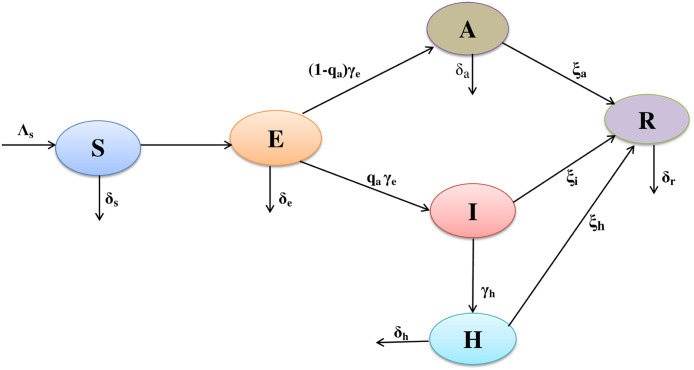
In the underlying dynamic model, the total population $N\left(t\right)$ is classified into six sub-populations (classes), namely susceptible $S\left(t\right)$, exposed $E\left(t\right)$, asymptomatic $A\left(t\right)$, clinically ill or symptomatic $I\left(t\right)$, hospitalized $H\left(t\right)$ and recovered $R\left(t\right)$, respectively. A schematic representation of the above biological mechanism of coronavirus in human upon which our model is based is shown in Fig. 1. The dynamics of novel coronavirus model is governed by the following system of nonlinear ordinary differential equations:

Fig. 1.

Schematic representation of the model. The schematic flow diagram represents the biological mechanism of the novel coronavirus (COVID-19) infection in India, which influences the formulation of the mathematical model (7). The mathematical model consists of six sub-populations: susceptible $S\left(t\right)$, exposed $E\left(t\right)$, asymptomatic $A\left(t\right)$, symptomatic or clinically ill $I\left(t\right)$, hospitalized or isolated $H\left(t\right)$ and recovered $R\left(t\right)$ individuals in a total population of $N\left(t\right)=S\left(t\right)$ + $E\left(t\right)$ + $A\left(t\right)$ + $I\left(t\right)$ + $H\left(t\right)$ + $R\left(t\right)$ individuals.

Dynamics of susceptible individuals $S\left(t\right)$

The susceptible individual is recruited into the population with a constant inflow rate ${\Lambda }_s$ and decreased by a natural mortality rate ${\delta }_s$. Here, ${\beta }_s{\alpha }_a$ represents the transmission coefficient of the susceptible to exposed individuals, ${\beta }_s{\alpha }_i$ is the transmission coefficient of symptomatic infected classes to the susceptible, and ${\beta }_s{\alpha }_h$ denotes transmission coefficient of the hospitalized classes to susceptible population. We consider ${\beta }_s$ is the disease transmission coefficient for both the infectiousness of COVID-19 and contact rates, with adjustment factors ${\alpha }_a$ (for asymptomatic classes), ${\alpha }_i$ (for symptomatic classes) and ${\alpha }_h$ (for hospitalized individuals).

Albeit, coronavirus is supposed to be spread completely by symptomatic populations, a very lower rate of transmission by asymptomatic populations cannot even be ruled out. The adjustment parameter ${\alpha }_a\ge 0$ take into accounts for varying levels of hygiene preventions through asymptomatic, an analogous explanation can be drawn to the adjustment parameters ${\alpha }_i$ and ${\alpha }_h$ during symptomatic and hospitalization, respectively. As the asymptomatic, symptomatic and hospitalization programmes and hygiene preventions during asymptomatic, symptomatic and hospitalization were executed and enriched progressively after an epidemic of coronavirus, the spreading coefficients ${\alpha }_a{\beta }_s$, ${\alpha }_i{\beta }_s$ and ${\alpha }_h{\beta }_s$, asymptomatic, symptomatic and hospitalized rates could be modeled as a time-dependent parameters in computations. Moreover, the interplay among susceptible and infected population (asymptomatic, symptomatic and hospitalized) is modeled utilizing standard homogeneous mixing incidence [52], [53], in the form of total individuals $N$. The rate of change of susceptible individuals can be represented by the following ordinary differential equation (ODE):

$$\frac{dS}{dt}={\Lambda }_s-\frac{{\beta }_{s}S({\alpha }_{a}A+{\alpha }_{i}I+{\alpha }_{h}H)}{N}-{\delta }_{s}S.$$ (1)

Dynamics of exposed individuals $E\left(t\right)$

The population who are exposed individuals but not yet developed clinical symptoms of coronavirus. The exposed individual is decreased by asymptomatic individuals at the rate ${\gamma }_e$ and natural death at the rate ${\delta }_e$. The constant per-capita rate ${\gamma }_e$ modeled progression from the exposed individuals $\left(E\right)$ to either the asymptomatic individuals $\left(A\right)$ or symptomatic individuals $\left(I\right)$; the constant $q_a(0<q_a<1)$ represents budget for the rate of progress of population who move to either the asymptomatic partially-infectious class $\left(A\right)$ or symptomatic class $\left(I\right)$ at the per-capita rate ${\gamma }_e$. The corresponding model dynamics for exposed population can be presented by the following ODE:

$$\frac{dE}{dt}=\frac{{\beta }_{s}S({\alpha }_{a}A+{\alpha }_{i}I+{\alpha }_{h}H)}{N}-{\delta }_{e}E-{\gamma }_{e}E.$$ (2)

Dynamics of asymptomatic individuals $A\left(t\right)$

Asymptomatic populations were exposed to the coronavirus but not infectious for the community. The exposed classes move to the asymptomatic classes at the rate ${\gamma }_e$ by a constant portion $(1-q_a)$. The asymptotic individuals progress to the recovered class at the per-capita rate ${\xi }_a$ and natural mortality rate ${\delta }_a$. The rate of change of asymptomatic individuals is governed by the following ODE:

$$\frac{dA}{dt}=(1-q_a){\gamma }_{e}E-{\delta }_{a}A-{\xi }_{a}A.$$ (3)

Dynamics of symptomatic individuals $I\left(t\right)$

The symptomatic individuals are produced after the progression of clinical symptoms of coronavirus (diagnosed by the clinicians) by the asymptomatic individuals. The exposed individuals move to the symptomatic classes at the per-capita rate ${\gamma }_e$ by a constant portion $q_a$. The symptomatic or clinically ill individuals progress to the hospitalized or isolated class $\left(H\right)$ at the per-capita rate ${\gamma }_i$ and natural mortality rate ${\delta }_i$. It can be assumed that ${\gamma }_i$, the per-capita rate at which symptomatic or clinically ill classes seek clinical attention and are therefore put into the hospitalized class, is bigger than ${\gamma }_e$, the per-capita rate at which the exposed individuals progress to the asymptomatic classes. The clinically ill classes (class $I$) are moved to the recover classes without being diagnosed at the per-capita rate ${\xi }_i$. The transmission dynamics of symptomatic populations are governed by the following ODE:

$$\frac{dI}{dt}=q_a{\gamma }_{e}E-{\delta }_{i}I-{\xi }_{i}I-{\gamma }_{i}I.$$ (4)

Dynamics of hospitalized individuals $H\left(t\right)$

These are the populations who have progressed clinical symptoms for coronavirus and have been isolated at the hospital for medical treatment. The hospitalized individuals are came from the clinically ill classes or symptomatic community (class $I$) at the per-capita rate ${\gamma }_i$ and it has natural mortality rate ${\delta }_h$. Hospitalized or isolated populations recover at the per-capita rate ${\xi }_h$. We assumed that ${\xi }_h>{\xi }_i$, as an hospitalized populations are likely to obtain a partially efficacious during isolation or hospitalization. The dynamics of hospitalized individuals are modeled by the following ODE:

$$\frac{dH}{dt}={\gamma }_{i}I-{\delta }_{h}H-{\xi }_{h}H.$$ (5)

Dynamics of recovered individuals $R\left(t\right)$

It can be assumed that the recovered population have enduring immunity against coronavirus. The asymptomatic, symptomatic and hospitalized individuals recovered from the coronavirus at the per-capita rates ${\xi }_a$, ${\xi }_i$ and ${\xi }_h$, respectively. The recovered individuals die at the per-capita rate ${\delta }_r$. The rate of change of recovered individuals can be written by the following ODE:

$$\frac{dR}{dt}={\xi }_{a}A+{\xi }_{i}I+{\xi }_{h}H-{\delta }_{r}R.$$ (6)

Based on the above biological assumptions and schematic representation of coronavirus (see Fig. 1) together with specific forms, we formulate a mathematical model of novel coronavirus given by the following six-dimensional nonlinear system of ODEs:

$$\left\{\begin{array}{c}\frac{dS}{dt}={\Lambda }_s-\frac{{\beta }_{s}S({\alpha }_{a}A+{\alpha }_{i}I+{\alpha }_{h}H)}{N}-{\delta }_{s}S,\hfill \\ \frac{dE}{dt}=\frac{{\beta }_{s}S({\alpha }_{a}A+{\alpha }_{i}I+{\alpha }_{h}H)}{N}-{\delta }_{e}E-{\gamma }_{e}E,\hfill \\ \frac{dA}{dt}=(1-q_a){\gamma }_{e}E-{\delta }_{a}A-{\xi }_{a}A,\hfill \\ \frac{dI}{dt}=q_a{\gamma }_{e}E-{\delta }_{i}I-{\xi }_{i}I-{\gamma }_{i}I,\hfill \\ \frac{dH}{dt}={\gamma }_{i}I-{\delta }_{h}H-{\xi }_{h}H,\hfill \\ \frac{dR}{dt}={\xi }_{a}A+{\xi }_{i}I+{\xi }_{h}H-{\delta }_{r}R,\hfill \end{array}\right)$$ (7)

the model is satisfied the following nonnegative initial conditions:

$$S\left(0\right)=S_0,E\left(0\right)=E_0,A\left(0\right)=A_0,I\left(0\right)=I_0,H\left(0\right)=H_0,R\left(0\right)=R_0.$$ (8)

Since the model system (7) monitors the dynamics of human population, all state variables are assumed to be positive.

Basic reproduction number

The basic reproduction number, symbolized by $R_0$, is ‘the expected number of secondary cases produced, in a completely susceptible population, by a typical infective individual’s [54], [55]. The dimensionless basic reproduction number provides a threshold, which play a crucial role in determining the disease persists or dies out from the population. In a more general way $R_0$ can be stated as the number of new infections created by a typical infective population at an infection free equilibrium. $R_0<1$ determines on an average an infected population creates less than one new infected population during the course of its infective period, and the infection can die out. In reverse way, $R_0>1$ determines each infected population creates, on an average, more than one new infection, and the disease can spread over the population. The basic reproduction number $R_0$ can be computed by using the concept of next generation matrix [54], [55]. In order to do this, we consider the nonnegative matrix $\mathcal{F}$ and the non-singular $M-$matrix $\mathcal{V}$, expressing as the production of new-infection and transition part respectively, for the system (7), are described by

$$\mathcal{F}=\left[\begin{array}{c}\hfill \frac{S}{N}{\beta }_s({\alpha }_{a}A+{\alpha }_{i}I+{\alpha }_{h}H)\hfill \\ \hfill 0\hfill \\ \hfill 0\hfill \\ \hfill 0\hfill \end{array}\right],\mathcal{V}=\left[\begin{array}{c}\hfill ({\delta }_e+{\gamma }_e)E\hfill \\ \hfill -(1-q_a){\gamma }_{e}E+({\delta }_a+{\xi }_a)A\hfill \\ \hfill -q_a{\gamma }_{e}E+({\delta }_i+{\xi }_i+{\gamma }_i)I\hfill \\ \hfill -{\gamma }_{i}I+({\delta }_h+{\xi }_h)H\hfill \end{array}\right].$$

The Jacobian matrix for the system (7), can be computed at an infection free state $(E=A=I=H=0)$, we have

$$F=\left[\begin{array}{cccc}\hfill 0\hfill & \hfill {\beta }_s{\alpha }_a\hfill & \hfill {\beta }_s{\alpha }_i\hfill & \hfill {\beta }_s{\alpha }_h\hfill \\ \hfill 0\hfill & \hfill 0\hfill & \hfill 0\hfill & \hfill 0\hfill \\ \hfill 0\hfill & \hfill 0\hfill & \hfill 0\hfill & \hfill 0\hfill \\ \hfill 0\hfill & \hfill 0\hfill & \hfill 0\hfill & \hfill 0\hfill \end{array}\right],$$

$$V=\left[\begin{array}{cccc}\hfill {\delta }_e+{\gamma }_e\hfill & \hfill 0\hfill & \hfill 0\hfill & \hfill 0\hfill \\ \hfill -(1-q_a){\gamma }_e\hfill & \hfill ({\delta }_a+{\xi }_a)\hfill & \hfill 0\hfill & \hfill 0\hfill \\ \hfill -q_a{\gamma }_e\hfill & \hfill 0\hfill & \hfill ({\delta }_i+{\xi }_i+{\gamma }_i)\hfill & \hfill 0\hfill \\ \hfill 0\hfill & \hfill 0\hfill & \hfill -{\gamma }_i\hfill & \hfill ({\delta }_h+{\xi }_h)\hfill \end{array}\right].$$

The basic reproduction number $R_0=\rho \left(F{V}^{-1}\right)$, where $\rho \left(F{V}^{-1}\right)$ represents the spectral radius for a next generation matrix $F{V}^{-1}$. Thus, from the system (7), we get the basic reproduction number $R_0$ is

$$R_0=\frac{(1-q_a){\gamma }_e{\beta }_s{\alpha }_a}{({\delta }_e+{\gamma }_e)({\delta }_a+{\xi }_a)}+\frac{q_a{\gamma }_e{\beta }_s{\alpha }_i}{({\delta }_e+{\gamma }_e)({\delta }_i+{\xi }_i+{\gamma }_i)}$$$$+\frac{q_a{\beta }_s{\alpha }_h{\gamma }_e{\gamma }_i}{({\delta }_e+{\gamma }_e)({\delta }_i+{\xi }_i+{\gamma }_i)({\delta }_h+{\xi }_h)}.$$ (9)

Equilibria

The system (7) has two biologically feasible equilibrium points, which are as follows:

• 1.disease-free equilibrium point $E^0({\Lambda }_s∕{\delta }_s,0,0,0,0,0)$,
• 2.
  endemic equilibrium point $E^{\ast }(S^{\ast },E^{\ast },A^{\ast },I^{\ast },H^{\ast },R^{\ast })$, where

  $$S^{\ast }=\frac{1}{{\delta }_s}\left[{\Lambda }_s-\frac{({\delta }_e+{\gamma }_e)({\delta }_i+{\xi }_i+{\gamma }_i)}{q_a{\gamma }_e}\right],$$

  $$E^{\ast }=\frac{{\delta }_i+{\xi }_i+{\gamma }_i}{q_a{\gamma }_e}{I}^{\ast },H^{\ast }=\frac{{\gamma }_i}{{\delta }_h+{\xi }_h}{I}^{\ast },$$

  $$A^{\ast }=\frac{({\delta }_i+{\xi }_i+{\gamma }_i)(1-q_a)}{q_a({\delta }_a+{\xi }_a)}{I}^{\ast },$$

  $$R^{\ast }=\frac{1}{{\delta }_r}\left[{\xi }_i+\frac{{\xi }_a(1-q_a)({\delta }_i+{\xi }_i+{\gamma }_i)}{q_a({\delta }_a+{\xi }_a)}+\frac{{\xi }_h{\gamma }_i}{{\delta }_h+{\xi }_h}\right]I^{\ast },$$

  $$I^{\ast }=\frac{{\Lambda }_s(R_0-1)}{{\delta }_s}\times \left[1+\frac{{\xi }_i}{{\delta }_r}+\frac{({\delta }_e+{\gamma }_e)({\delta }_i+{\xi }_i+{\gamma }_i)(R_0-1)}{q_a{\gamma }_e{\delta }_s}+\frac{{\delta }_i+{\xi }_i+{\gamma }_i}{q_a{\gamma }_e}+\left(1+\frac{{\xi }_a}{{\delta }_r}\right)\frac{{\gamma }_e({\delta }_i+{\xi }_i+{\gamma }_i)(1-q_a)}{\left(q_a{\gamma }_e\right)({\delta }_a+{\xi }_a)}+\left(1+\frac{{\xi }_h}{{\delta }_r}\right)\frac{{\gamma }_i}{{\delta }_h+{\xi }_h}\right]{}^{-1}.$$

The disease-free equilibrium point $E^0$ is always feasible and the endemic equilibrium point $E^{\ast }$ feasible only if $R_0>1$ and ${\Lambda }_s>\left(1+\frac{{\delta }_e}{{\gamma }_e}\right)\left(\frac{{\delta }_i+{\xi }_i+{\gamma }_i}{q_a}\right)$.

Model calibration and coronavirus data source

A detailed elucidation on the computer simulations for the coronavirus model system (7) is investigated in this section. We start by building up on the parameter estimations followed by some computer simulation results, which provide insights on the eradication and development of the dynamics of novel coronavirus (COVID-19) epidemic. Parameter values are taken from literature and some of the parameters are estimated from the observed data. List of the parameter values with description are given in Table 2 and the values of the remaining parameters estimated from the observed data from five different states of India, namely Kerala, Andhra Pradesh, West Bengal, Maharashtra, Karnataka including India, which are given in Table 3. The initial population sizes for different states, namely Kerala, Maharashtra, Andhra Pradesh, West Bengal, Karnataka and the Republic of India are stated in Table 5. Also the recruitment rate ${\Lambda }_s$ for five different states and overall India are listed in Table 5.

Table 2.

Table of biologically relevant parameter values and their description for the coronavirus model system (7).

Parameter	Biological meaning	Values (Unit)	Source
${\Lambda }_s$	Inflow rate of susceptible individual	–	–
${\beta }_s$	Disease transmission coefficient	${\mathrm{day}}^{-1}$	Estimated
${\alpha }_a$	Adjustment factor for asymptomatic classes	0.20 (0, 1)	[7]
${\alpha }_i$	Adjustment factor for symptomatic classes	0.45 (0, 1)	[28]
${\alpha }_h$	Adjustment factor for hospitalized individuals	(0, 1)	Estimated
${\delta }_s$	Natural death rate of susceptible classes	0.1945 $\times 10^{-4}{\mathrm{day}}^{-1}$	[56]
${\delta }_e$	Mortality rate of exposed individuals	0.1945 $\times 10^{-4}{\mathrm{day}}^{-1}$	[56]
${\delta }_a$	Mortality rate of asymptomatic individuals	0.1945 $\times 10^{-4}{\mathrm{day}}^{-1}$	[56]
${\delta }_i$	Mortality rate of symptomatic individuals	0.018  ${\mathrm{day}}^{-1}$	[57]
${\delta }_h$	Mortality rate of hospitalized individuals	0.1945 $\times 10^{-4}{\mathrm{day}}^{-1}$	[56]
${\delta }_r$	Mortality rate of recovered individuals	0.1945 $\times 10^{-2}{\mathrm{day}}^{-1}$	[56]
${\gamma }_e$	Conversion rate from exposed to asymptomatic individuals	1/7  ${\mathrm{day}}^{-1}$	[1]
${\gamma }_i$	Rate at which symptomatic individuals become hospitalized	${\mathrm{day}}^{-1}$	Estimated
$q_a$	Proportion of exposed individuals	(0, 1)	Estimated
${\xi }_a$	Rate of recovery from asymptomatic individuals	${\mathrm{day}}^{-1}$	Estimated
${\xi }_i$	Rate of recovery from symptomatic individuals	${\mathrm{day}}^{-1}$	Estimated
${\xi }_h$	Rate of recovery from hospitalized individuals	${\mathrm{day}}^{-1}$	Estimated

Table 3.

Estimated parameter values from the daily confirmed and cumulative confirmed coronavirus observed data.

Parameters	India	Kerala	Andhra Pradesh	West Bengal	Maharashtra	Karnataka
${\beta }_s$	0.879	0.899	1.221	1.799	1.021	0.879
${\xi }_a$	0.302	0.341	0.876	0.241	0.359	0.128
$q_a$	0.710	0.146	0.439	0.091	0.551	0.291
${\xi }_h$	0.114	0.010	0.102	0.471	0.269	0.130
${\gamma }_i$	0.201	0.389	0.862	0.469	0.010	0.481
${\xi }_i$	0.210	0.211	0.209	0.210	0.211	0.209
${\alpha }_h$	0.350	0.349	0.351	0.349	0.350	0.349

Table 5.

Estimated values of the initial population size and the constant inflow rate for the five provinces of India and the Republic of India.

Parameters	India	Kerala	Andhra Pradesh	West Bengal	Maharashtra	Karnataka	Source
$S\left(0\right)$	160 000	400 000	130 000	120 000	1 000 000	200 000	Estimated
$E\left(0\right)$	250	800	1000	1000	1700	1600	Estimated
$A\left(0\right)$	10	100	100	100	250	150	Estimated
$I\left(0\right)$	1	1	1	1	2	1	Data
$H\left(0\right)$	1	1	1	1	1	1	Estimated
$R\left(0\right)$	0	0	0	0	0	0	Data
$M\left(0\right)$	0	0	0	0	0	0	Estimated
${\Lambda }_s$	35 000	13 000	19 000	21 000	20 000	21 000	Estimated

Power-law growth in observed COVID-19 data

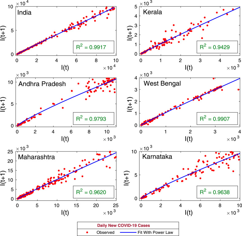
Initially, we perform a simple analysis to observe some insight of the ongoing COVID-19 pandemic. We investigated the relationship between the infected population of ${(t+n)}^{th}$ and $t$th day, with time lag of $n$th days. Considering $n=1$, we have plotted the infected populations of $t$th days and ${(t+1)}^{th}$ days along the horizontal and vertical axis respectively, in Fig. 2. The infected population follows the power law

$$X_{t+1}=\alpha {X_t}^{\beta },$$ (10)

where $X_t$ is the number of symptomatic infected cases on $t$th day; $X_{t+1}$ is the number of symptomatic infected cases on ${(t+1)}^{th}$ day, and $\alpha$ and $\beta$ are parameters. The values of $\alpha$, $\beta$ and coefficient of determination $\left(R^2\right)$ for the five states of India, namely, Kerala, Andhra Pradesh, West Bengal, Maharashtra, Karnataka and the Republic of India are listed in Table 1. The value of $R^2$ is very close for all the provinces and the curve $X_{t+1}=\alpha {X_t}^{\beta }$ fits perfectly with the observed COVID-19 cases for all the provinces. Population with power law growth provides essential information about the future growth of the population. Hence, the preliminary analysis of the observed COVID-19 cases using power law method is most relevant. The exponent $\beta$ is different for different provinces and the list for all the provinces are given in Table 1, which is listed as $\beta$ decreasing. The Republic of India has largest exponent comparing to its five states. Out of the five states, Kerala has lowest number of reported COVID-19 cases but Kerala has second large exponent, followed by Maharashtra, West Bengal, Karnataka and Andhra Pradesh.

Fig. 2.

Power law growth. The figure represents the recurrence plots for the daily new coronavirus cases for five provinces of India, namely, Kerala, Andhra Pradesh, West Bengal, Maharashtra, Karnataka and the Republic of India. Solid blue curves are the best fit of the power law of the kind (10). The coefficient of determination $\left(R^2\right)$ for each provinces are shown in the inset. The trend of power law shows that the best fit curves are increasing for all the provinces of India as well as overall India.

Table 1.

Parameter values and coefficient of determination $\left(R^2\right)$ for the power law $X_{t+1}=\alpha {X_t}^{\beta }$, and the corresponding curve fitting has been shown in the Fig. 2.

Provinces	$\alpha$	$\beta$	$R^2$
India	1.456	0.9672	0.9919
Kerala	1.479	0.9522	0.9429
Maharashtra	1.676	0.9466	0.9620
West Bengal	1.556	0.9451	0.9907
Karnataka	3.316	0.8653	0.9638
Andhra Pradesh	3.616	0.8591	0.9793

PRCC sensitivity analysis

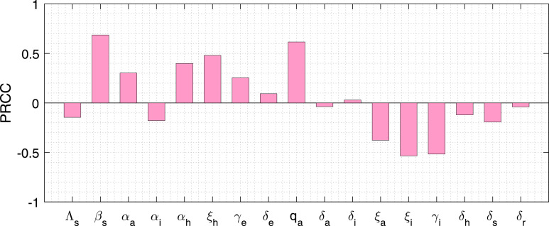
To identify the most sensitive parameters with respect to symptomatic individuals, we performed a sensitivity analysis by using Partial Rank Correlation Coefficient (PRCC) technique for all the input parameters against the variable $I$. The set of most sensitive parameters, which have the ability to reduce the outbreak of coronavirus diseases, can be estimated from the available data from different states (Kerala, Maharashtra, Andhra Pradesh, Karnataka, West Bengal) as well as the Republic of India. In our coronavirus system (7) has 17 parameters for which we varied all the system parameters simultaneously. PRCC quantifies the relationship among a state equation of interest and each of model parameters. As a result PRCC aid to obtain the important parameters, which contribute most to the system variability. For model simulation, we consider the PRCC values between −1.0 and +1.0.

Following the method established by Marino et al. [58], we performed Latin hypercube sampling and generated 2800 samples to compute the PRCC and the p-values with reference to the symptomatic classes at the day 60. The Fig. 3 designates the PRCC results, which implies that the highest positively correlated parameters are the disease transmission coefficient rate ${\beta }_s$, proportion rate of exposed individuals $q_a$, the rate ${\xi }_h$ by which the hospitalized class converted to recovered class, the rate ${\alpha }_h$ by which susceptible individuals converted to exposed class and the highly negatively correlated parameters are the rate ${\xi }_i$ by which symptomatic individuals become recovered, the rate ${\gamma }_i$ by which symptomatic individuals converted to hospitalized class, and the rate ${\xi }_a$ by which the asymptomatic individuals moved to recovered individuals, account for most uncertainty with respect to the symptomatic population. Thus, our PRCC analysis yields these 7 parameters ${\beta }_s$, $q_a$, ${\xi }_i$, ${\gamma }_i$, ${\xi }_h$, ${\alpha }_h$ and ${\xi }_a$ are the most effective parameters out of 17 parameters. Therefore, we have estimated the 7 parameters by using least square method.

Fig. 3.

Parameter Sensitivity. Partial rank correlation coefficients illustrating the dependence of symptomatic individuals $I$ on each of the system parameters at the day 60 with $p<0.02$.

Parameter estimation

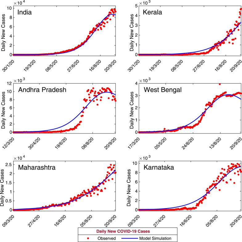
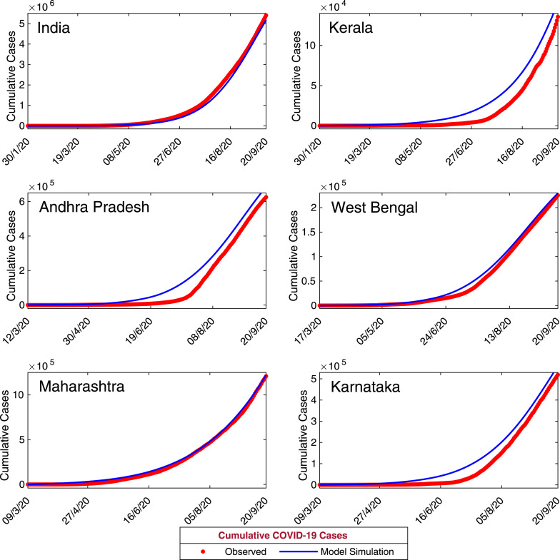
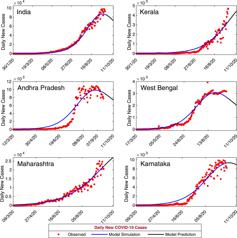
Now, we have calibrated our coronavirus disease model (7) with daily confirmed new coronavirus cases for the entire India and five states namely, Kerala, Andhra Pradesh, West Bengal, Maharashtra and Karnataka. Data of daily confirmed new coronavirus cases for whole India obtained from World Health Organization (WHO) situation report for the period January 30, 2020–September 20, 2020. Data of daily confirmed new coronavirus cases for the states, Kerala, Andhra Pradesh, West Bengal, Maharashtra and Karnataka were obtained from India COVID-19 Tracker (https://www.covid19india.org/). First COVID-19 patient identified in Kerala on January 30, 2020. Hence we have collected COVID-19 data for Kerala and for entire India for the period January 30, 2020–September 20, 2020. First COVID-19 patient identified in West Bengal on March 17, 2020 and the data obtained for West Bengal for the period March 17, 2020–September, 20, 2020. COVID-19 data for Andhra Pradesh obtained for the period March 12, 2020–September 20, 2020. Also, the COVID-19 data for Maharashtra and Karnataka were obtained for the period March 9, 2020–September 20, 2020. We fit our coronavirus model system (7) with daily new coronavirus cases (class I in the model) for the five states (Andhra Pradesh, Kerala, West Bengal, Maharashtra and Karnataka) and for India. Also, the cumulative coronavirus cases has been fitted with our model system. The observed data were fitted in Matlab using least squares method and we have estimated the parameters ${\beta }_s$, ${\xi }_a$, $q_a$, ${\xi }_h$, ${\gamma }_i$, ${\xi }_i$ and ${\alpha }_h$ as these parameters found more sensitive in the PRCC analysis [59]. The biological interpretations of the model parameters are given in Table 2. The estimated values of the model parameters for all the data sets are given in Table 3. The initial population sizes for all the data sets are also estimated to match with the confirmed new coronavirus cases (see Table 5). The output of our model for daily new cases are shown in Fig. 4. Also, the observed daily new coronavirus cases are overlapped on Fig. 4. It is also important to observe that the total number of coronavirus cases in a province. So, the observed daily cumulative confirmed coronavirus cases and the model simulation has been plotted in the Fig. 5.

Fig. 4.

Model estimation based on observed data. Daily new confirmed positive coronavirus cases for India and five states of India, namely, Kerala, Andhra Pradesh, West Bengal, Maharashtra and Karnataka. Observed data are shown in red circles, whereas the blue curve is the best fitting curve of the model system (7). The parameter values are used for numerical simulation and listed in Table 2, Table 3. The initial population sizes used for numerical simulation are listed in Table 5.

Fig. 5.

Model estimation based on observed data. Daily cumulative confirmed coronavirus cases for India and five states of India, namely, Kerala, Andhra Pradesh, West Bengal, Maharashtra and Karnataka. Observed data points are shown in red circles, whereas the blue curve is the best fitting curve of the model system (7). The parameter values used for numerical simulation are listed in Table 2, Table 3. The initial population sizes used for numerical simulation are listed in Table 5. (For interpretation of the references to color in this figure legend, the reader is referred to the web version of this article.)

To assure the performance of our coronavirus system (7), we have computed Mean Absolute Error $\left(E_{MAE}\right)$ and Root Mean Square Error $\left(E_{RMSE}\right)$. Here, $E_{MAE}$ and $E_{RMSE}$ are given by

$$E_{MAE}=\frac{{\Sigma }_{i=1}^n|O\left(i\right)-Q\left(i\right)|}{n},$$

$$E_{RMSE}=\sqrt{\frac{{\Sigma }_{i=1}^n{(O\left(i\right)-Q\left(i\right))}^2}{n}},$$

where $O\left(i\right)$ represents the observed value, $Q\left(i\right)$ is the model output and $n$ is the sample size of the observed data. The values of $E_{MAE}$ and $E_{RMSE}$ for the five states (Kerala, Andhra Pradesh, West Bengal, Maharashtra and Karnataka) and the Republic of India are presented in Table 4.

Table 4.

Accuracy of the COVID-19 model (7) for the five different states of India and the Republic of India.

Performance Metrics	India	Kerala	Andhra Pradesh	West Bengal	Maharashtra	Karnataka
$E_{MAE}$	2339.5	172.9	894.7	151.2	858.8	594.1
$E_{RMSE}$	3861.2	287.5	1235.8	219.2	1346.5	771.3

The fitting data enables us to quantify the basic reproduction number $R_0$ from the expression of (9). The basic reproduction number for coronavirus in different states, for Kerala, $R_0=3.3870$; Andhra Pradesh, $R_0=1.8155$; West Bengal, $R_0=1.5525$; Maharashtra, $R_0=1.2937$; Karnataka, $R_0=1.5934$ and for India, $R_0=1.6795$. Let us observe that the basic reproduction is relatively high in Kerala, relative to the other four states and the overall India considered here. From the basic reproduction number $R_0$ in overall India, it can be concluded that the coronavirus outbreaks is pandemic and the Govt. should take a necessary action to keep social distancing and necessary precautions. The basic reproduction number $R_0$ for five provinces and overall India are presented Table 6.

Table 6.

Basic reproduction number of the five different provinces of India and the Republic of India.

Reproduction Number	India	Kerala	Andhra Pradesh	West Bengal	Maharashtra	Karnataka
$R_0$	1.6795	3.3870	1.8155	1.5525	1.2937	1.5934

From the data fitting, it can be observed that our model performs relatively good in all the states namely, Kerala, Andhra Pradesh, West Bengal, Maharashtra and Karnataka. This is showing a good agreement with the observed data and curve fitting with the coronavirus disease model (7) under consideration. However, the model performance less well in the case of whole India as the number of confirmed coronavirus cases is relatively high. Though, the increasing trend of the daily confirmed coronavirus cases have been nicely captured by the model for all the data sets. We have also computed the numerical errors for computing the numerical simulations for our model and the corresponding lowest value of $E_{MAE}$ and $E_{RMSE}$ have been obtained for the state West Bengal, since the size of the data is lower than the other data sets (see Table 4).

Transcritical bifurcation

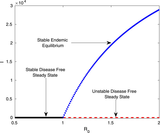
The coronavirus model system (7) undergoes transcritical bifurcation at $R_0=1$. In Fig. 6, we have plotted the symptomatic individuals $\left(I\right)$ in the $(R_0,I)$ plane. The basic reproduction number, $R_0$ increased gradually by increasing the disease transmission coefficient ${\beta }_s$ from 0.25 to 1.1 and then $R_0$ changes from 0.5 to 2.0. The system parameters value are considered as $q_a=0.71$, ${\xi }_a=0.302$, ${\gamma }_i=0.20$ and ${\xi }_h=0.114$, ${\Lambda }_s=35000$ and other parameters are listed in Table 2. The Fig. 6 clearly shows that the system (7) experiences transcritical bifurcation at $R_0=1$. The black line in Fig. 6 represents the stable disease free equilibrium point $\left(E_0\right)$, the red dashed line represents the unstable endemic equilibrium point $\left(E^{\ast }\right)$ and the blue curve represents the stable branch of the endemic equilibrium point $\left(E^{\ast }\right)$. Hence, the endemic equilibrium point $\left(E^{\ast }\right)$ is stable for $R_0>1$ and unstable for $R_0<1$. Also the disease free equilibrium point $\left(E_0\right)$ is stable for $R_0<1$ and unstable for $R_0>1$. As the endemic equilibrium point $E^{\ast }$ is stable for $R_0>1$, so the coronavirus disease will spread in the population when $R_0>1$.

Fig. 6.

Transcritical bifurcation. The figure shows the transcritical bifurcation diagram of the system (7) with respect to the basic reproduction number $R_0$. The stability of the system (7) interchange at the threshold $R_0=1$. The parameters values are ${\Lambda }_s=35000$, $q_a=0.710$, ${\xi }_a=0.302$, ${\gamma }_i=0.201$, ${\xi }_h=0.114$ and other parameters are listed in Table 2, Table 3. (For interpretation of the references to color in this figure legend, the reader is referred to the web version of this article.)

Short-term prediction

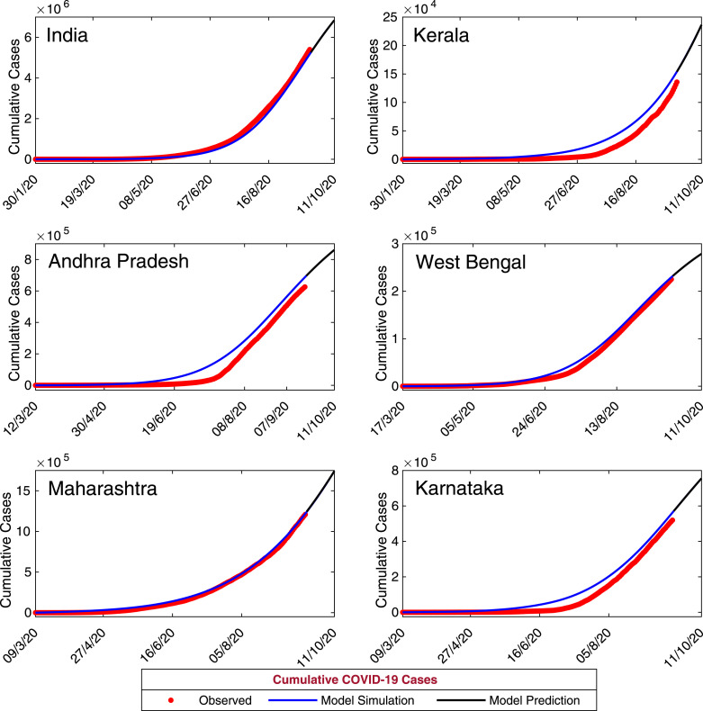
Due to absence of any effective vaccine or treatment strategies for novel coronavirus, predictive mathematical models can aid in understanding the complicated dynamics of coronavirus transmission and its control as well as its intricate epidemiological cycle. In order to study the short term prediction for our model system (7), we have simulated the daily and cumulative symptomatic classes of coronavirus cases for the time period September 21, 2020 to October 11, 2020 using the estimated parameters values in Table 3 with initial population sizes in Table 5. The other baseline parameter values are specified in Table 2. The simulated results for the period September 21, 2020 to October 11, 2020 for the five provinces of India, namely Kerala, Andhra Pradesh, West Bengal, Maharashtra and Karnataka and the Republic of India have shown in Fig. 7 and Fig. 8, respectively. The black solid curves are the model prediction. The predicted daily confirmed new coronavirus cases are increasing for the states Kerala and Maharashtra whereas for all other provinces the daily confirmed new coronavirus cases are decreasing. The predicted cumulative coronavirus cases for all the provinces are increasing; as the predicted daily new coronavirus cases are positive.

Fig. 7.

Model-Based Data-Driven short-term prediction. Model simulations shows the short term predictions for the five provinces of India, namely Kerala, Andhra Pradesh, West Bengal, Maharashtra, Karnataka and the Republic of India. The solid black curve represents the model predictions for the daily new infected coronavirus cases. The baseline parameter values are listed in Table 2 and rest of estimated parameters are listed in Table 3.

Fig. 8.

Model-Based Data-Driven short-term prediction. Model simulations shows the short term predictions for the five provinces of India, namely Kerala, Andhra Pradesh, West Bengal, Maharashtra, Karnataka and the Republic of India. The solid black curve represents the model predictions for the new infected cumulative coronavirus cases. The baseline parameter values are listed in Table 2 and rest of estimated parameters are listed in Table 3.

Sensitivity analysis for $R_0$

To describe how best to diminish human impermanency and morbidity due to novel coronavirus, it is very essential to see the relative significance of various factors responsible for its transmission. The initial disease transmission is completely associated to the reproduction number $R_0$, and we calculate the sensitivity indices with regard to $R_0$, to the parameters for the system (7). The sensitivity indices describe us whether or not the infectious diseases will develop throughout the individuals. Sensitivity analysis is mainly utilized to describe the robustness of the reproduction number $R_0$ to fluctuation in the system parameters. It also give us to identify the relative change in a state variable when a system parameter alters. The normalized forward sensitivity index for $R_0$ with respect to the parameter $p$ is defined as follows:

$${\Gamma }_p^{R_0}=\frac{\partial R_0}{\partial p}\times \frac{p}{R_0}.$$

As we have the explicit expression for $R_0$ in (9), we obtain the analytical formulae for sensitivity indices of $R_0$, ${\Gamma }_p^{R_0}$, to each of fourteen parameters stated in Table 7.

Table 7.

Table of sensitivity indices of basic reproduction number $R_0$ for the coronavirus model system (7) for five different states of India and the Republic of India. The baseline parameter values taken from the Table 2 and other parameters are estimated and taken from the Table 3.

Parameters	Sensitivity Indices
	India	Kerala	Andhra Pradesh	West Bengal	Maharashtra	Karnataka
${\beta }_s$	1.00000	1.00000	1.00000	1.00000	1.00000	1.00000
${\alpha }_a$	0.10061	0.13384	0.08572	0.88393	0.19764	0.61277
${\alpha }_i$	0.38041	0.02776	0.12057	0.05795	0.77989	0.10000
${\alpha }_h$	0.51899	0.83839	0.79371	0.05813	0.02247	0.28723
$q_a$	0.65308	0.84328	0.84692	0.01786	0.56080	0.13695
${\gamma }_e$	0.13613$\times 10^{-3}$	0.13613$\times 10^{-3}$	0.13613$\times 10^{-3}$	0.13613$\times 10^{-3}$	0.13613$\times 10^{-3}$	0.13613$\times 10^{-3}$
${\gamma }_i$	0.11017	0.30263	0.07796	−0.01874	−0.95085$\times 10^{-2}$	0.02940
${\delta }_e$	−0.13613$\times 10^{-3}$	−0.13613$\times 10^{-3}$	−0.13613$\times 10^{-3}$	−0.13613$\times 10^{-3}$	−0.13613$\times 10^{-3}$	−0.13613$\times 10^{-3}$
${\delta }_a$	−0.64789$\times 10^{-5}$	−0.76561$\times 10^{-5}$	−0.19033$\times 10^{-5}$	−0.71629$\times 10^{-4}$	−0.10678$\times 10^{-4}$	−0.93098$\times 10^{-4}$
${\xi }_a$	−0.10060	−0.13384	−0.08572	−0.88386	−0.19763	−0.61267
${\delta }_i$	−0.06132	−0.04121	−0.02491	−0.49065$\times 10^{-2}$	−0.09594	−0.01611
${\xi }_i$	−0.42926	−0.28918	−0.17362	−0.03430	−0.67444	−0.11329
${\delta }_h$	−0.88531$\times 10^{-4}$	−0.16275$\times 10^{-2}$	−0.15132$\times 10^{-3}$	−0.24053$\times 10^{-5}$	−0.16186$\times 10^{-5}$	−0.42968$\times 10^{-4}$
${\xi }_h$	−0.51890	−0.83677	−0.79356	−0.05812	−0.02247	−0.28719

As for example, the sensitivity index of $R_0$ with regards to ${\beta }_s$ is

$${\Gamma }_{{\beta }_s}^{R_0}=\frac{\partial R_0}{\partial {\beta }_s}\times \frac{{\beta }_s}{R_0}=1,$$

independent of any parameters. This represents that $R_0$ is the increasing function with respect to ${\beta }_s$. It implies that the probability of disease transmission has a high impact on coronavirus control and management. Other parameters have their sensitivity indices are specified in Table 7.

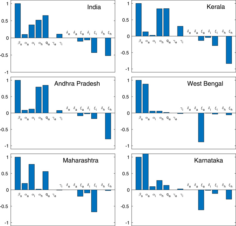
From Table 7, it can be noticed that some of the indices are positive and some of the indices are negative, which indicate that the indices having ‘+’ signs increase the value of $R_0$ as one increase them and those having ‘-’ signs decrease the value of $R_0$, as they are increased. The most sensitive parameter is the disease transmission coefficient ${\beta }_s$, where sensitivity index ${\Gamma }_{{\beta }_s}^{R_0}=1$ indicates that the increasing ${\beta }_s$ by 10% will increase $R_0$ by 10%. Also, the sensitivity index of ${\xi }_a$, that is, ${\Gamma }_{{\beta }_s}^{R_0}=-0.844286$ represents that increasing ${\xi }_a$ by 10% will decrease $R_0$ by 8.44286%. Similarly, we can interpret the other parameters too.

We plot the sensitivity indices of $R_0$, for each of the model parameters using in Table 7 has been shown in Fig. 9. In order to control the coronavirus outbreaks, we must target the most sensitive parameters who has the great impact in controlling the system dynamics. For instance, the disease transmission coefficient ${\beta }_s$ is the most effective parameter in controlling the coronavirus diseases, which can easily be identified from Fig. 9 as well as in Table 7.

Fig. 9.

Normalized forward sensitivity indices of$R_0$. Result shows the normalized forward sensitivity indices of the basic reproduction number $R_0$ for the five provinces of India, namely Kerala, Andhra Pradesh, West Bengal, Maharashtra, Karnataka and the Republic of India, with respect to each of the baseline parameter values using in Table 7.

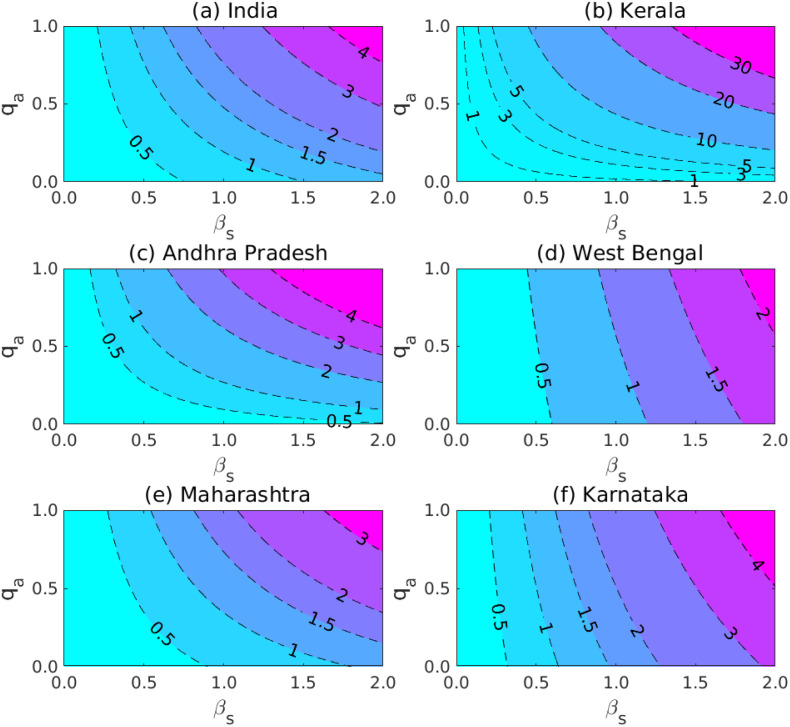
To control the coronavirus outbreaks, contour plots has been drawn for the $R_0$ with respect to the positively correlated parameters, namely disease transmission coefficient ${\beta }_s$ and the clinical outbreak rate $q_a$ for all the infected classes in Fig. 10. The contour plot represents the dependence of $R_0$ for the five states (Kerala, Andhra Pradesh, West Bengal, Maharashtra, Karnataka) and the Republic of India. Contour plot indicates that for the higher values of ${\beta }_s$ and $q_a$ the basic reproduction number $R_0$ become high, which means the coronavirus may enter the stage-3 and it spread through the community. Therefore, to control $R_0$ must be restrict the values of the transmission coefficient ${\beta }_s$ and the portion $q_a$ by which the exposed class become symptomatically ill. To keep the mortality rate as low as possible, we must be take the values of ${\beta }_s$ and $q_a$ as small as possible. The Fig. 9 and Table 7 represents that the adjustment factors ${\alpha }_a$, ${\alpha }_i$ and ${\alpha }_h$ are positively correlated with the basic reproduction number $R_0$. Thus, we must have to reduce the adjust factors too. Thus, we may conclude that to reduce the coronavirus disease outbreaks we need to maintain social distancing, limit or stop taking fairs and theater performances etc.

Fig. 10.

Contour plots of basic reproduction number$R_0$. Contour plots of basic reproduction number $R_0$ for the five different provinces of India and the Republic of India. Plot contours of $R_0$ versus the disease transmission coefficient ${\beta }_s$ and the portion $q_a$ of exposed class after being clinically ill due to novel coronavirus. For (a) the Republic of India, (b) the province Kerala, (c) Andhra Pradesh, (d) West Bengal (e) Maharashtra and (f) Karnataka. The contour plots exhibits that the higher disease transmission probability of coronavirus disease will remarkably increase the basic reproduction number $R_0$.

The baseline parameter values are obtained from Table 2 and rest of the parameter values are estimated and obtained from Table 3.

Long-term dynamics

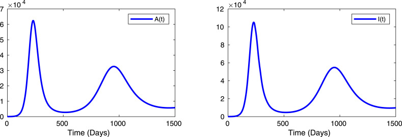
To study the future outbreak of coronavirus diseases, we simulate our system (7) for a long days of the infected individuals, namely asymptomatic individuals and symptomatic or clinically ill individuals for the parameters are listed in Table 2 and we have considered the estimated parameters for Table 3 in case of Indian data only with initial population sizes are as follows: S(0)=1600000, E(0)=250, A(0)=10, I(0)=1, H(0)=1 and R(0)=0. The model simulation represented that the people from overall India can experience future epidemics if the control policies are not implemented more effectively, as shown in Fig. 11. The number of infected individuals (asymptomatic and symptomatic) are oscillate around 235 days and around 950 days. This can be interpreted as the reproduction number $R_0$ is always greater than unity in India (see Table 6 for India). The factors like low air temperature and as well as low humidity has a great impact on the transmission dynamics of novel coronavirus [11].

Fig. 11.

Long term dynamics. Long term dynamics for the coronavirus disease system (7) for the infectious individuals (asymptomatic and symptomatic populations). The value of the parameters used for the numerical simulation is given in Table 2, Table 3. The other parameters values are ${\beta }_s=0.879$, ${\gamma }_i=0.201$, $q_a=0.710$, ${\xi }_a=0.302$, ${\xi }_h=0.114$ and ${\Lambda }_s=35000$ with the initial conditions: $S\left(0\right)=1600000$, $E\left(0\right)=250$, $A\left(0\right)=10$, $I\left(0\right)=1$, $H\left(0\right)=1$, $R\left(0\right)=0$.

Discussion and conclusion

According to the INDIA COVID-19 TRACKER report, 61,48,640 confirmed cases, 51,01,118 recovered cases and 96,378 confirmed deaths due to novel coronavirus outbreaks in India [60], as of September 29, 2020. The total number of new cases and new deaths are occurred everyday reported from different cities across the India [60]. This is a terrifying circumstances as India has approximately 139 crores population and may enter stage-3 of coronavirus disease transmission. Till date, there is no specific vaccine, antivirals or effective therapeutics to treat coronavirus diseases. During this period, forecasting is the utmost priority for the planning of health care and control the novel coronavirus diseases. Thus, mathematical modeling can aid us in designing to control the outbreak of coronavirus diseases in absence of any treatment or any specific diagnostic test.

In this manuscript, we proposed a compartmental epidemic model to study the transmission dynamics of novel coronavirus diseases and its short-term prediction as well as long-term dynamics. In our proposed model, we consider two infectious individuals, namely asymptomatic and symptomatic individuals with former being a fast spreader of the coronavirus diseases. Our model formulation is based on the work by Gumel et al. [7], where we estimate the system parameters based on the PRCC sensitivity analysis with the data from five states of India and overall India, in which the number of cumulative classes grow exponentially.

We calibrated the proposed model to fit with the data from five different states of India, namely Maharashtra, Karnataka, Kerala, Andhra Pradesh, West Bengal and the Republic of India. The most important part is to perform the sensitivity analysis of 17 model parameters and its estimation. To identify the key input parameters which contributed to the symptomatic outcome, strongly assisted the implementation of an integrated policy for various measures, involving the epidemic during different phases of the diseases, we use the sensitivity analysis by using PRCC techniques. PRCC analysis yields the most sensitive parameters are ${\beta }_s$, $q_a$, ${\gamma }_i$, ${\alpha }_h$, ${\xi }_a$ and ${\xi }_h$ out of 17 input parameters. Then we estimated these 7 parameters based on the data from five different states of India and from the overall India. By fitting data on novel coronavirus cases during January 30, 2020 to September 20, 2020, in the five different states of India and the overall India to our proposed model, we were able to get estimates of the unknown parameters for our system.

By fitting our proposed model system (7) with real data obtained from India COVID-19 Tracker (https://www.covid19india.org/), we were able to get acceptable estimations for the system parameters and curve fitting, as shown in Fig. 4, Fig. 5. To ensure the performance of our system, we compute the numerical errors, namely $E_{MAE}$ and $E_{RMSE}$. Within the reasonable set of parameter values, we obtained relatively good fits to novel coronavirus data, as plotted in Fig. 4 and Fig. 5, respectively.

From the basic reproduction number $R_0$ in Table 6, it can be compared that the province Kerala is highly effective by coronavirus diseases compare to other four provinces of India and the Republic of India. Nevertheless, our model-based analysis also demonstrates that the basic reproduction number in India and five different provinces of India remains greater than unity. The estimation of basic reproduction number $R_0$ indicates that the strengthen control involvements are mandatory to reduce and/or eradicate the future coronavirus diseases. Thus, in this scenario the public must have to give utmost priority to stay home quarantine and maintain the social distancing to combat against coronavirus pandemic.

From the sensitivity indices (see Table 7 and Fig. 9) for the basic reproduction number $R_0$, we observed that the disease transmission coefficient ${\beta }_s$ and the portion $q_a$ clinical outbreak rates in all infected classes are positively correlated with $R_0$. This indicates that to reduce coronavirus diseases the social distancing is the most important factor and we reduce the values for ${\beta }_s$ and $q_a$ to control the diseases. As we know, for $R_0<1$ the diseases can be died out. Thus, to keep control the value of $R_0$ we must reduce ${\beta }_s$ and $q_a$. While investigating the contour plot, we observe that for the lower values for ${\beta }_s$ and $q_a$, the reproduction number can be controlled and reduced to less than unity, as shown in Fig. 10. Thus, if we are able to control the social distancing, then we are able to control the basic reproduction number $R_0$ and hence we are able to eradicate the coronavirus diseases. Since $R_0$ quantifies the initial epidemic transmission, its sensitivity indices enable us to establish the relative significance of various parameters in coronavirus transmission. From the sensitivity of basic reproduction number $R_0$, we can conclude that the most effective control measures are the isolation of all close contacts and strengthening the self-protection ability for susceptible individuals.

We have checked our calibrated epidemic model for the short term prediction in the five provinces of India and the republic of India. The simulation of our calibrated model successfully able to capture the increasing growth patterns for five different provinces, namely Karnataka, Kerala, Andhra Pradesh, Maharashtra, West Bengal and the Republic of India. In order to study the long-term dynamics of our model, we observed the most interesting switching phenomena, as plotted in Fig. 11.

Our model simulation and prediction suggests that the novel coronavirus diseases has a potentiality to exhibit oscillatory dynamics in the future but can be controlled by maintaining social distances and effectiveness of isolation or hospitalization. Our model forecasts that isolation or hospitalization of populations with coronavirus symptoms, under stringent hygiene safeguards and social distancing, be able to effectual control in a community and may even eliminate the diseases. Our study also suggests that the size and duration of an epidemic can be considerably affected by timely implementation of the hospitalization or isolation programme. Based on the model simulations and prediction to control the coronavirus diseases, we provide some particular inferences to face with emerging diseases:

i.

avoidance of mass gatherings, rallies, social distancing and implement extensive lock-down;

ii.

provide essential personal safeguard to the staff who are involved in emergency services;

iii.

timely give the statistics of the coronavirus diseases to the community, including the number of asymptomatic cases, symptomatic cases, hospitalized cases and so on.

Future expansion of this research can consider some other classes like dead class to make the model more realistic. This COVID-19 model can be apply to other provinces to provide the forecasting of the pandemic. Our future research can also consider applying optimal control theory to provide decision makers with better policies of controlling the spread of the COVID-19. This COVID-19 model can also be use to study other infected disease system.

CRediT authorship contribution statement

Subhas Khajanchi: Conceptualization, Writing - original draft, Software, Investigation, Validation, Writing - review & editing. Kankan Sarkar: Conceptualization, Writing - original draft, Software, Formal analysis, Investigation. Jayanta Mondal: Conceptualization, Writing - original draft, Software, Formal analysis, Validation. Kottakkaran Sooppy Nisar: Software, Methodology, Validation, Writing - review & editing. Sayed F. Abdelwahab: Validation, Writing - review & editing, Funding acquisition.

Declaration of Competing Interest

The authors declare that they have no known competing financial interests or personal relationships that could have appeared to influence the work reported in this paper.

Data availability

All data supporting the findings of this study are in the paper and available from the corresponding author on reasonable request.

References

- 1.2020. Coronavirus disease (COVID-19) outbreak situation.https://www.who.int/emergencies/diseases/novel-coronavirus -2019. [Google Scholar]
- 2.Zhu N. A novel coronavirus from patients with pneumonia in china, 2019. N Engl J Med. 2019;382:727–733. doi: 10.1056/NEJMoa2001017. [DOI] [PMC free article] [PubMed] [Google Scholar]
- 3.Fuk-Woo C.J. Novel coronavirus indicating person-to-person transmission: a study of a family cluster. Lancet. 2019;395(2020):514–523. doi: 10.1016/S0140-6736(20)30154-9. [DOI] [PMC free article] [PubMed] [Google Scholar]
- 4.Cohen J., Normile D. New SARS-like virus in China triggers alarm. Science. 2020;367:234–235. doi: 10.1126/science.367.6475.234. [DOI] [PubMed] [Google Scholar]
- 5.Tang B., Wang X., Li Q., Bragazzi N.L., Tang S., Xiao Y. Estimation of the transmission risk of the 2019-ncov and its implication for public health interventions. J Clin Med. 2020;9(2):462. doi: 10.3390/jcm9020462. [DOI] [PMC free article] [PubMed] [Google Scholar]
- 6.Chen Y., Liu Q., Guo D. Emerging coronaviruses: Genome structure, replication, and pathogenesis. J Med Virol. 2020;92:418–423. doi: 10.1002/jmv.25681. [DOI] [PMC free article] [PubMed] [Google Scholar]
- 7.Gumel A.B., Ruan S., Day T., Watmough J., Brauer F., den Driessche P. Van. Modelling strategies for controlling sars outbreaks. Proc R Soc Lond B. 2004;271:2223–2232. doi: 10.1098/rspb.2004.2800. [DOI] [PMC free article] [PubMed] [Google Scholar]
- 8.Drosten C., Günther S., Preiser W., Werf S., Brodt H., Becker S. Identification of a novel coronavirus in patients with severe acute respiratory syndrome. N Engl J Med. 2003;348:1967–1976. doi: 10.1056/NEJMoa030747. [DOI] [PubMed] [Google Scholar]
- 9.Zhou P. A pneumonia outbreak associated with a new coronavirus of probable bat origin. Nature. 2020;579:270–273. doi: 10.1038/s41586-020-2012-7. [DOI] [PMC free article] [PubMed] [Google Scholar]
- 10.2020. Centers for disease control and prevention. Coronavirus disease 2019 (COVID-19)https://www.cdc.gov/coronavirus/2019-ncov/index.html [Google Scholar]
- 11.Jingyuan W., Ke T., Kai F., Weifeng L. 2020. High temperature and high humidity reduce the transmission of COVID-19. [DOI] [Google Scholar]
- 12.Khajanchi S., Sarkar K., Mondal J. 2020. Dynamics of the COVID-19 pandemic in India. arXiv preprint arXiv:2005.06286. [Google Scholar]
- 13.2020. Event horizon - COVID- 19. Coronavirus COVID=19 global risk assessment.http://rocs.hu-berlin.de/corona/relative-import-risk [Google Scholar]
- 14.2020. National centre for disease control. Travel advisory.https://ncdc.gov.in/WriteReadData/l892s/63950984511580999086.pdf [Google Scholar]
- 15.2020. National centre for disease control. COVID-19 outbreak in China.https://ncdc.gov.in/WriteReadData/l892s/34827556791580715701.pdf [Google Scholar]
- 16.Bhargava B., Suda n P. 2020. Prepared for the coronavirus. The Hindu.https://www.thehindu.com/opinion/op-ed/prepared-for-the-coronavirus/article30785312.ece [Google Scholar]
- 17.Ferguson N.M. Imperial college COVID-19 response team. 2020. Impact of non-pharmaceutical interventions (NPIs) to reduce COVID- 19 mortality and healthcare demand; pp. 1–20.https://www.imperial.ac.uk/media/imperial-college/medicine/sph/ide/gida-fellowships/Imperial-College-COVID19-NPI-modelling-16-03-2020.pdf [DOI] [PMC free article] [PubMed] [Google Scholar]
- 18.Khajanchi S., Bera S., Roy T.K. Mathematical analysis of the global dynamics of a HTLV-I infection model, considering the role of cytotoxic T-lymphocytes. Math Comput Simulation. 2021;180:354–378. [Google Scholar]
- 19.Anderson R.M., Heesterbeek H., Klinkenberg D., Hollingsworth T.D. How will country-based mitigation measures influence the course of the COVID-19 epidemic? Comment. 2020;395:931–934. doi: 10.1016/S0140-6736(20)30567-5. [DOI] [PMC free article] [PubMed] [Google Scholar]
- 20.Egger M., Johnson L., Althaus C., Schöni A., Salanti G., Low N. Developing WHO guidelines: Time to formally include evidence from mathematical modelling studies. F1000Research. 2017;6:1584. doi: 10.12688/f1000research.12367.1. [DOI] [PMC free article] [PubMed] [Google Scholar]
- 21.Khajanchi S., Banerjee S. Stability and bifurcation analysis of delay induced tumor immune interaction model. Appl Math Comput. 2014;248:652–671. [Google Scholar]
- 22.Khajanchi S. Stability analysis of a mathematical model for glioma-immune interaction under optimal therapy. Int J Nonlinear Sci Numer Simul. 2019;20(3–4):269–285. [Google Scholar]
- 23.Khajanchi S. Uniform persistence and global stability for a brain tumor and immune system interaction. Biophys Rev Lett. 2017;12(4):187–208. [Google Scholar]
- 24.Khajanchi S. Modeling the dynamics of glioma-immune surveillance. Chaos Solitons Fractals. 2018;114:110–118. [Google Scholar]
- 25.Chen T., Rui J., Wang Q., Zhao Z., Cui J., Yin L. A mathematical model for simulating the phase-based transmissibility of a novel coronavirus. Infect Dis Poverty. 2020;9:24. doi: 10.1186/s40249-020-00640-3. [DOI] [PMC free article] [PubMed] [Google Scholar]
- 26.Imai N. 2020. Estimating the potential total number of novel coronavirus cases in Wuhan City, China.https://www.preventionweb.net/news/view/70092 [Google Scholar]
- 27.Liu Z., Magal P., Seydi O., Webb G. 2020. Predicting the cumulative number of cases for the COVID-19 epidemic in China from early data.arXiv:2002.12298 [DOI] [PubMed] [Google Scholar]
- 28.Nadim S.K., Ghosh I., Chattopadhyay J. 2020. Short-term predictions and prevention strategies for COVID-2019: A model based study.arXiv:2003.08150 [DOI] [PMC free article] [PubMed] [Google Scholar]
- 29.Tang B., Bragazzi N.L., Li Q., Tang S., Xiao Y., Wu J. An updated estimation of the risk of transmission of the novel coronavirus (2019-nCov) Infect Dis Model. 2020;5:248–255. doi: 10.1016/j.idm.2020.02.001. [DOI] [PMC free article] [PubMed] [Google Scholar]
- 30.Wu J.T., Leung K., Leung G.M. Nowcasting and forecasting the potential domestic and international spread of the 2019-nCoV outbreak originating in Wuhan, China: a modelling study. Lancet. 2020;395:689–697. doi: 10.1016/S0140-6736(20)30260-9. [DOI] [PMC free article] [PubMed] [Google Scholar]
- 31.Khajanchi S. Chaotic dynamics of a delayed tumor-immune interaction model. Int J Biomath. 2020;13(2) [Google Scholar]
- 32.Sarkar K., Khajanchi S. Impact of fear effect on the growth of prey in a predator–prey interaction model. Ecol Complex. 2020;42 [Google Scholar]
- 33.Giordano G., Blanchini F., Bruno R., Colaneri P., Di Filippo A., Di Matteo A. Modelling the COVID-19 epidemic and implementation of population-wide interventions in Italy. Nat Med. 2020;26:855–860. doi: 10.1038/s41591-020-0883-7. [DOI] [PMC free article] [PubMed] [Google Scholar]
- 34.Kucharski A.J., Russell T.W., Diamond C., Liu Y., Edmunds J., Funk S. Eggo RM early dynamics of transmission and control of COVID-19: A mathematical modelling study. Lancet Infect Dis. 2020;20:553–558. doi: 10.1016/S1473-3099(20)30144-4. [DOI] [PMC free article] [PubMed] [Google Scholar]
- 35.Eikenberry S.E., Muncuso M., Iboi E., Phan T., Kostelich E., Kuang Y. To mask or not to mask: Modeling the potential for face mask use by the general public to curtail the COVID-19 pandemic. Infect Dis Model. 2020;5:293–308. doi: 10.1016/j.idm.2020.04.001. [DOI] [PMC free article] [PubMed] [Google Scholar]
- 36.Gatto M., Bertuzzo E., Mari L., Miccoli S., Carraro L., Casagrandi R. Spread and dynamics of the COVID-19 epidemic in Italy: effects of emergency containment measures. Proc Natl Acad Sci USA. 2020;117(19):10484–10491. doi: 10.1073/pnas.2004978117. [DOI] [PMC free article] [PubMed] [Google Scholar]
- 37.Ngonghala C.N., Iboi E., Eikenberry S., Scotch M., Gumel A.B. Mathematical assessment of the impact of non-pharmaceutical interventions on curtailing the 2019 novel coronavirus. Math Biosci. 2019;325 doi: 10.1016/j.mbs.2020.108364. [DOI] [PMC free article] [PubMed] [Google Scholar]
- 38.Arino J., Brauer F., van den Driessche P., Watmough J., Wu J. Simple models for containment of a pandemic. J R Soc Interface. 2006;3:453–457. doi: 10.1098/rsif.2006.0112. [DOI] [PMC free article] [PubMed] [Google Scholar]
- 39.Das A., Dhar A., Kundu A., Goyal S. 2020. Covid-19: analysis of a modified SEIR model, a comparison of different intervention strategies and projections for India. [DOI] [PMC free article] [PubMed] [Google Scholar]
- 40.Shekatkar S. 2020. INDSCI-SIM: A state-level epidemiological model for India.https://indscicov.in/indscisim [Google Scholar]
- 41.Agrawal S et al. COVID-19 epidemic: unlocking the lockdown in India (working paper). IISc-TIFR technical report,https://covid19.iisc.ac.in/wp-content/uploads/2020/04/Report-1-20200419-UnlockingTheLockdownInIndia.pdf.
- 42.Khajanchi S., Sarkar K. Forecasting the daily and cumulative number of cases for the COVID-19 pandemic in india. Chaos. 2020;30 doi: 10.1063/5.0016240. [DOI] [PMC free article] [PubMed] [Google Scholar]
- 43.Sarkar K., Khajanchi S., Nieto J.J. Modeling and forecasting of the COVID-19 pandemic in India. Chaos Solitons Fractals. 2020;139 doi: 10.1016/j.chaos.2020.110049. [DOI] [PMC free article] [PubMed] [Google Scholar]
- 44.Samui P., Mondal J., Khajanchi S. A mathematical model for COVID-19 transmission dynamics with a case study of India. Chaos Solitons Fractals. 2020;140 doi: 10.1016/j.chaos.2020.110173. [DOI] [PMC free article] [PubMed] [Google Scholar]
- 45.Chatterjee K., Chatterjee K., Kumar A., Shankar S. Healthcare impact of Covid-19 epidemic in India: A stochastic mathematical model. Med J Armed Forces India. 2020;76:147–155. doi: 10.1016/j.mjafi.2020.03.022. [DOI] [PMC free article] [PubMed] [Google Scholar]
- 46.Rai R.K., Khajanchi S., Tiwari P.K., Venturino E., Misra A.K. Impact of social media advertisements on the transmission dynamics of COVID-19 pandemic in India. J Appl Math Comput. 2021 doi: 10.1007/s12190-021-01507-y. [DOI] [PMC free article] [PubMed] [Google Scholar]
- 47.Perc M., Miksic N.G., Slavinec M., A. Stozer. Forecasting COVID- -19. Front Phys. 2020;8:127. [Google Scholar]
- 48.Das D.K., Khajanchi S., Kar T.K. The impact of the media awareness and optimal strategy on the prevalence of tuberculosis. Appl Math Comput. 2020;366 [Google Scholar]
- 49.Das D.K., Khajanchi S., Kar T.K. Transmission dynamics of tuberculosis with multiple re-infections. Chaos Solitons Fractals. 2020;130 [Google Scholar]
- 50.Khajanchi S., Das D.K., Kar T.K. Dynamics of tuberculosis transmission with exogenous reinfections and endogenous reactivation. Physica A. 2018;497:52–71. [Google Scholar]
- 51.Das D.K., Khajanchi S., Kar T.K. 2019 8th international conference on modeling simulation and applied optimization. IEEE; 2019. Influence of multiple re-infections in tuberculosis transmission dynamics: a mathematical approach; pp. 1–5. [DOI] [Google Scholar]
- 52.Anderson R.M., May R.M. Oxford University Press; 1991. Infectious diseases of humans. [Google Scholar]
- 53.Diekmann O., Heesterbeek JAP. Wiley; New York: 2000. Mathematical epidemiology of infectious diseases: model building, analysis and interpretation. [Google Scholar]
- 54.Diekmann O., Heesterbeek J.S.P., Metz JAJ. On the definition and the computation of the basic reproduction ratio in models for infectious diseases in heterogeneous populations. J Math Biol. 1990;28:365–382. doi: 10.1007/BF00178324. [DOI] [PubMed] [Google Scholar]
- 55.van den Driessche P., Watmough J. Reproduction numbers and subthreshold endemic equilibria for compartmental models of disease transmission. Math Biosci. 2002;180:29–48. doi: 10.1016/s0025-5564(02)00108-6. [DOI] [PubMed] [Google Scholar]
- 56.2020. Open government data (OGD) platform India or data.gov.in.https://data.gov.in/resources/crude-death-rate-india-2011 [Google Scholar]
- 57.2020. Coronavirus disease 2019 (COVID-19): WHO situation report; p. 46.https://www.who.int/docs/default-source/coronaviruse/situation-reports/20200306-sitrep-46-covid-19.pdf?sfvrsn=96b04adf-2 [Google Scholar]
- 58.Marino S., Hogue I.B., Ray C.J., Kirschner D.E. A methodology for performing global uncertainty and sensitivity analysis in systems biology. J Theoret Biol. 2008;254:178–196. doi: 10.1016/j.jtbi.2008.04.011. [DOI] [PMC free article] [PubMed] [Google Scholar]
- 59.Banerjee S., Khajanchi S., Chaudhuri S. A mathematical model to elucidate brain tumor abrogation by immunotherapy with T11 target structure. PLoS One. 2015;10(5) doi: 10.1371/journal.pone.0123611. [DOI] [PMC free article] [PubMed] [Google Scholar]
- 60.2020. India covid- 19 tracker.https://www.covid19india.org/ [Google Scholar]
Associated Data
This section collects any data citations, data availability statements, or supplementary materials included in this article.
Data Availability Statement