Time-dependent probability distribution for number of infection in a stochastic SIS model: case study COVID-19

Abstract

We derive the time-dependent probability distribution for the number of infected individuals at a given time in a stochastic Susceptible-Infected-Susceptible (SIS) epidemic model. The mean, variance, skewness, and kurtosis of the distribution are obtained as a function of time. We study the effect of noise intensity on the distribution and later derive and analyze the effect of changes in the transmission and recovery rates of the disease. Our analysis reveals that the time-dependent probability density function exists if the basic reproduction number is greater than one. It converges to the Dirac delta function on the long run (entirely concentrated on zero) as the basic reproduction number tends to one from above. The result is applied using published COVID-19 parameters and also applied to analyze the probability distribution of the aggregate number of COVID-19 cases in the United States for the period: January 22, 2020-March 23, 2021. Findings show that the distribution shifts concentration to the right until it concentrates entirely on the carrying infection capacity as the infection growth rate increases or the recovery rate reduces. The disease eradication and disease persistence thresholds are calculated.

1. Introduction

Several advances have been made in the field of mathematical modeling in studying the behavior of certain dynamical systems whose state evolves with time [1], [10], [23], [38], [43], [44], [49], [51], [54], [56], [57]. Most of these dynamical processes in nature are far from equilibrium and so using stationary distribution to describe and analyze the evolution of such processes has a great limitation [8], [9], [30], [55]. Although studying the evolution of such random dynamical systems using time-dependent probability density function is challenging, significant analysis and estimates about the process can be deduced from such study. The exact solutions in terms of probability density function of dynamical systems can only be obtained for a restricted class of dynamical systems [12], [13], [21], [31], [41].

Apart from Fokker-Planck equation (FPE), a partial differential equation that describes the time evolution of probability density function, there are other methods such as the moment or cumulant equations approach [17] that can be used to analyze the distribution of nonlinear systems under random perturbations. Because of the complexity of solving partial differential equations, many approximate methods have been developed numerically to solve the FPE equation for situations far from equilibrium. A simple thermodynamically consistent matrix numerical method (MNM) is developed by Holubec et al. [26] for solving over-damped FPEs with time-dependent coefficients. Paola at al. [17] proposed an approximate method called the Taylor moments for the probabilistic description of response of nonlinear system driven by a stochastic process. Other methods such as the stochastic linearization (SL) method [53], the equivalent non-linear equations method (ENLE) [14], the moment differential equation method (MDE) Monte Carlo simulation using a non-Gaussian closure approximation [40], the path integral approach, perturbation technique and Galerkin method [32], [35], [60] have been developed for approximating the time-dependent probability density of some general first-order and second-order non-linear stochastic systems.

In this work, we develop the time-dependent probability density function for the number of infections of certain diseases satisfying a particular stochastic SIS epidemic model. The state transition probability density function for the dynamic process is governed by the FPE equation [19], [58]. The result obtained is used to analyze the distribution of the aggregate daily infection count of COVID-19 cases for the United States collected from the Center of Disease Control and Prevention (CDC) for the period: 01/22/2020-03/23/2021.

The organization of the paper is as follows. In Section 2, we formulate a stochastic differential equation (SDE) used in modeling the number of infection at a given time by extending the well known deterministic SIS epidemic model with vital dynamics to a stochastic case. The existence and uniqueness of the solution of the SDE is also discussed. The threshold under which the disease dies out using the SDE model is obtained and analyzed. In Section 3, we derive the closed form time-dependent probability density function for the number of infection at a given time $t$ for the stochastic SIS model. Properties of the distribution, namely, mean, variance, skewness, kurtosis functions are also derived in Section 3. Special cases of the distribution are also discussed in this section. Numerical results are carried out in Section 4 to verify our claim. Discussion and summary of the work done are presented in Section 5.

2. Formulation of model

Our main focus in this work is on the derivation of time-dependent probability density function for the number of infected individuals following the general stochastic SIS model. To do this, we first study the SIS deterministic epidemic model

$$\begin{array}{ccc}d\mathcal{S}\hfill & =\hfill & (\Lambda \mathcal{N}-\frac{\mathit{\beta }\mathcal{S}\mathcal{I}}{\mathcal{N}}-\mu \mathcal{S}+\gamma \mathcal{I})dt,\mathcal{S}\left(t_0\right)={\mathcal{S}}_0,\hfill \\ d\mathcal{I}\hfill & =\hfill & (\frac{\mathit{\beta }\mathcal{S}\mathcal{I}}{\mathcal{N}}-(\mu +\gamma )\mathcal{I})dt,\mathcal{I}\left(t_0\right)={\mathcal{I}}_0,\hfill \end{array}$$ (2.1)

where $\mathcal{I}$ and $\mathcal{S}$ represent the population of infected and susceptible individuals, respectively, ${\mathcal{S}}_0>0,$ ${\mathcal{I}}_0\ge 0,$ and $\Lambda >0$ is the recruitment rate, $\mathit{\beta }$ is the transmission rate, $\mu$ is the natural death rate and $\gamma$ is the temporary recovery rate. To maintain a constant population, we assume $\Lambda =\mu$. With this, the population size $\mathcal{N}$ remains constant over time so that $\mathcal{S}+\mathcal{I}=\mathcal{N}$. This reduces the model governing $\mathcal{I}$ in (2.1) to the form

$$d\mathcal{I}=(\frac{\mathit{\beta }}{\mathcal{N}}(\mathcal{N}-\mathcal{I})\mathcal{I}-(\mu +\gamma )\mathcal{I})dt,\mathcal{I}\left(t_0\right)={\mathcal{I}}_0.$$ (2.2)

The model (2.1) has been studied extensively by Brauer et al. [11], Hethcote and Yorke [25], Lajmanovich and Yorke [33] and Nold [45].

Many factors such as pneumonia seasonality, mobility, testing rates, mask use per capital weather [27], social behavior, strain-specific factors [42], and public health intervention [34] can act as external fluctuations affecting the contact/transmission rate of the disease. For this reason, we assume the contact/transmission rate $\mathit{\beta }$ of the disease is affected by environmental perturbations, such as stated above, changing the infection transmission rate $\mathit{\beta }$ to the form

$$\mathit{\beta }dt=\beta dt+\sigma dW\left(t\right),$$ (2.3)

where each infected individual makes $\mathit{\beta }dt$ infectious contacts with each other in the interval $[t,t+dt),$ $W\left(t\right)$ is a standard Wiener process on a filtered probability space ($\Omega ,{\mathcal{F}}_t,{\left({\mathcal{F}}_t\right)}_{t\ge 0},\mathbb{P}$), the filtration function ${\left({\mathcal{F}}_t\right)}_{t\ge 0}$ is right-continuous and each ${\mathcal{F}}_t$ with $t\ge 0$ contains all $\mathbb{P}$-null sets in ${\mathcal{F}}_t$. By substituting (2.3) into (2.1), we reduce the deterministic epidemic model (2.1) to the Stratonovich stochastic model

$$\{\begin{array}{ccc}d\mathcal{S}\hfill & =\hfill & (\mu \mathcal{N}-\frac{\beta \mathcal{S}\mathcal{I}}{\mathcal{N}}-\mu \mathcal{S}+\gamma \mathcal{I})dt-\frac{\sigma \mathcal{S}\mathcal{I}}{\mathcal{N}}\circ dW\left(t\right),\mathcal{S}\left(t_0\right)={\mathcal{S}}_0,\hfill \\ d\mathcal{I}\hfill & =\hfill & (\frac{\beta \mathcal{S}\mathcal{I}}{\mathcal{N}}-(\mu +\gamma )\mathcal{I})dt+\frac{\sigma \mathcal{S}\mathcal{I}}{N}\circ dW\left(t\right),\mathcal{I}\left(t_0\right)={\mathcal{I}}_0,\hfill \end{array}$$ (2.4)

where $\circ$ denotes the Stratonovich integral [2]. We used the Stratonovich calculus instead of the Itô calculus following the arguments made in [7], [37]. We also assume the initial process $({\mathcal{S}}_0,{\mathcal{I}}_0)$ is ${\mathcal{F}}_{t_0}$ measurable and independent of $W\left(t\right)-W\left(t_0\right)$. The solution of (2.4) with Itô calculus has been studied extensively by Gray [22]. In their work, Dalal et al. [16] showed that the introduction of stochastic noise can stabilize system that is unstable. In this work, we are interested in studying how the system behaves in the presence of noise in the transmission rate of the disease. This behavior is studied by analyzing the time-dependent probability density function of the process $\mathcal{S}\left(t\right)$ and $\mathcal{I}\left(t\right)$. The stochastic differential equation has a unique positive solution [22], [39], [47], [59] in the feasible region

$$\mathcal{T}:=\{(\mathcal{S},\mathcal{I})\in {\mathbb{R}}_{+}^2|0\le \mathcal{S}+\mathcal{I}\le \mathcal{N}\}$$ (2.5)

for all $t\ge 0$ with probability one.

The model governing $\mathcal{I}$ in (2.4) reduces to the Itô form

$$\begin{array}{ccc}\hfill d\mathcal{I}& =& (\frac{\beta }{\mathcal{N}}(\mathcal{N}-\mathcal{I})-(\mu +\gamma )+\frac{{\sigma }^2}{2{\mathcal{N}}^2}(\mathcal{N}-\mathcal{I})(\mathcal{N}-2\mathcal{I}))\mathcal{I}dt\hfill \\ & & +\frac{\sigma }{\mathcal{N}}(\mathcal{N}-\mathcal{I})\mathcal{I}dW\left(t\right),\mathcal{I}\left(t_0\right)={\mathcal{I}}_0.\hfill \end{array}$$ (2.6)

Define

$$\begin{array}{ccc}\hfill R_0& =& \frac{\beta }{\mu +\gamma },\hfill \\ \hfill {\mathcal{R}}_0& =& \frac{\beta +{\sigma }^2/2}{\mu +\gamma }.\hfill \end{array}$$ (2.7)

The number $R_0$ is referred to the reproduction number for (2.1). This is the average number of infection cases produced by an infectious individual when introduced into a completely susceptible population. The number ${\mathcal{R}}_0$ is the stochastic version of $R_0$ for the model (2.6).

It was shown in Méndez et al. [39] and Otunuga [48] that the boundaries $\mathcal{I}=0$ and $\mathcal{I}=\mathcal{N}$ of (2.6) are unattainable at all times if $R_0>1,$ regardless of the noise intensity. Following a similar Theorem in [22], we show in Theorem 1 that the disease will die out exponentially almost surely on the long run in the presence of noise if ${\mathcal{R}}_0\le 1$.

Theorem 1

For any given initial condition${\mathcal{I}}_0\in (0,\mathcal{N}),$the solution$\mathcal{I}\left(t\right)$of the stochastic differential Eq.(2.6)tends to zero exponentially almost surely if${\mathcal{R}}_0\le 1$.

Proof

It follows from (2.6) that

$$\begin{array}{ccc}\hfill d\ln \mathcal{I}& =& (\frac{\beta }{\mathcal{N}}(\mathcal{N}-\mathcal{I})-(\mu +\gamma )-\frac{{\sigma }^2}{2{\mathcal{N}}^2}(\mathcal{N}-\mathcal{I})\mathcal{I})dt\hfill \\ & & +\frac{\sigma }{\mathcal{N}}(\mathcal{N}-\mathcal{I})\mathcal{I}dW\left(t\right).\hfill \end{array}$$

If ${\mathcal{R}}_0\le 1,$ we have from (2.5) that

$$\begin{array}{ccc}\hfill \ln \mathcal{I}\left(t\right)& =& \ln {\mathcal{I}}_0+(\beta -(\mu +\gamma ))(t-t_0)-{\int }_{t_0}^t(\frac{\beta }{\mathcal{N}}+\frac{{\sigma }^2}{2{\mathcal{N}}^2}(\mathcal{N}-\mathcal{I}\left(s\right)))\mathcal{I}\left(s\right)\mathit{ds}\hfill \\ & & +\frac{\sigma }{\mathcal{N}}{\int }_{t_0}^t(\mathcal{N}-\mathcal{I}\left(s\right))\mathcal{I}\left(s\right)\mathit{dW}\left(s\right),\hfill \\ & <& \ln {\mathcal{I}}_0+(\mu +\gamma )({\mathcal{R}}_0-1)(t-t_0)+\frac{\sigma }{\mathcal{N}}{\int }_{t_0}^t(\mathcal{N}-\mathcal{I}\left(s\right))\mathcal{I}\left(s\right)\mathit{dW}\left(s\right),\hfill \\ & \le & \ln {\mathcal{I}}_0+\frac{\sigma }{\mathcal{N}}{\int }_{t_0}^t(\mathcal{N}-\mathcal{I}\left(s\right))\mathcal{I}\left(s\right)\mathit{dW}\left(s\right).\hfill \end{array}$$

The result follows from the fact that

$$\underset{t\to \infty }{lim\; sup}\frac{1}{t}\ln \left(\mathcal{I}\right(t\left)\right)<0,$$

using the large number theorem for martingales [24]. □

We see in Theorem 1 that replacing the condition ${\mathcal{R}}_0<1$ with the condition $R_0<1$ for the disease to die out exponentially almost surely is also valid. We note here that epidemic advances can still grow initially, leading to transient epidemic advance if

$$1-\frac{{\sigma }^2}{2(\mu +\gamma )}<R_0<1.$$

A numerical result is derived later in Section 4 to confirm Theorem 1 by showing that the stationary probability distribution of $\mathcal{I}$ concentrates entirely on zero if ${\mathcal{R}}_0\le 1$ (which also implies $R_0\le 1$). Likewise, it can be shown that the stochastic differential Eq. (3.2) has a unique stationary distribution if $R_0>1$. The proof of this is similar to the proof given in Theorem 6.2 of the work of Gray et al. [22], so we omit the proof here. We give the closed form representation of the time-dependent and stationary probability density function for $\mathcal{I}$ in the next section and confirm that these distributions exist if $R_0>1$.

It was shown in Otunuga [48] that the solution $\left(\mathcal{S}\right(t),\mathcal{I}(t\left)\right)$ of the system (2.4) is obtained as

$$\begin{array}{ccc}\hfill \mathcal{I}\left(t\right)& =& \frac{\mathcal{N}}{1+\overline{\mathcal{C}}(\frac{\mathcal{N}-{\mathcal{I}}_0}{\overline{\mathcal{C}}{\mathcal{I}}_0}\Phi (t,t_0)+\frac{{\sigma }^2}{2}\Phi (t,t_0){\int }_{t_0}^t{\Phi }^{-1}(s,t_0)ds)},\hfill \\ \hfill \mathcal{S}\left(t\right)& =& \mathcal{N}-\mathcal{I}\left(t\right),\hfill \end{array}$$ (2.8)

where

$$\Phi (t,t_0)=e^{-\frac{{\sigma }^2}{2}(\overline{\mathcal{A}}+1)(t-t_0)-\sigma (W\left(t\right)-W\left(t_0\right))},$$ (2.9)

and

$$\begin{array}{ccc}\hfill \overline{\mathcal{A}}& =& \frac{2}{{\sigma }^2}(\beta -(\mu +\gamma )-{\sigma }^2/2),\hfill \\ \hfill \overline{\mathcal{C}}& =& \frac{2}{{\sigma }^2}(\mu +\gamma ).\hfill \end{array}$$ (2.10)

Let $p_{\mathcal{I}}\left(\mathcal{I}\right|t,{\mathcal{I}}_0)$ be the probability density for the process $\mathcal{I}$ satisfying (2.6) at time $t$ given initial point ${\mathcal{I}}_0$. In his work, Otunuga [48] derived the probability density function $p_{\mathcal{I}}\left(\mathcal{I}\right|t,{\mathcal{I}}_0)$ for the specific case where the resulting Fokker Planck differential equation for $p_{\mathcal{I}}\left(\mathcal{I}\right|t,{\mathcal{I}}_0)$ has only discrete eigen-values $r\equiv r_n$ and $\lambda$ satisfying

$$\lambda =\frac{1}{{\sigma }^2}(\beta -(\mu +\gamma )-\sqrt{{(\beta -(\mu +\gamma \left)\right)}^2-2{\sigma }^{2}r}),$$

is a non-negative integer. In this work, we extend the work of Otunuga [48] to include both discrete and continuous eigen-values.

3. Derivation of time-dependent probability distribution for the general stochastic SIS epidemic model

Using the transformation

$$\begin{array}{ccc}\hfill S& =& \frac{\mathcal{S}}{\mathcal{N}},\hfill \\ \hfill I& =& \frac{\mathcal{I}}{\mathcal{N}},\hfill \end{array}$$ (3.1)

we reduce (2.4) to the form

$$\{\begin{array}{cc}dS=(\Lambda -\beta SI-\mu S+\gamma I)dt-\sigma SI\circ dW\left(t\right),\hfill & S\left(t_0\right)=S_0,\hfill \\ dI=(\beta SI-(\mu +\gamma \left)I\right)dt+\sigma SI\circ dW\left(t\right),\hfill & I\left(t_0\right)=I_0.\hfill \end{array}$$ (3.2)

By setting $S=1-I,$ the stochastic differential equation governing $I$ in (3.2) reduces to the Stratonovich stochastic differential equation

$$dI=\left(\beta \right(1-I)I-(\mu +\gamma \left)I\right)dt+\sigma (1-I)I\circ dW\left(t\right),I\left(t_0\right)=I_0.$$ (3.3)

The Itô equivalent of (3.3) is given by

$$\begin{array}{ccc}\hfill dI& =& (\beta (1-I)I-(\mu +\gamma )I+\frac{{\sigma }^2}{2}(1-I)I(1-2I))dt\hfill \\ & & +\sigma (1-I)I\circ dW\left(t\right),I\left(t_0\right)=I_0.\hfill \end{array}$$ (3.4)

Using the change of state variable

$$x=\frac{\overline{\mathcal{C}}I}{1-I}$$ (3.5)

in (3.4), we obtain the Itô stochastic differential equation

$$dx=\frac{{\sigma }^2}{2}x(\overline{\mathcal{A}}+2-x)dt+\sigma xdW\left(t\right),x\left(t_0\right)=x_0,$$ (3.6)

where $\overline{\mathcal{A}}$ and $\overline{\mathcal{C}}$ are defined in (2.10).

Let $p_X\left(x\right|t,x_0)$ be the probability density function for the process $x$ satisfying (3.6) at time $t$ given initial point $x_0,$ and let $p_X^s\left(x\right)$ denotes the corresponding limiting or stationary distribution. We give the closed form expression for $p_X^s\left(x\right)$ and $p_X\left(x\right|t,x_0)$ in the following theorem.

Theorem 2

Assume$x_0>0$and$\overline{\mathcal{A}}+1>0$. Then the solution$x\left(t\right)$satisfying(3.6)has a unique stationary and time-dependent probability density function$p_X^s\left(x\right)$and$p_X\left(x\right|t,x_0),$respectively, obtained as

$$\begin{array}{ccc}\hfill p_X^s\left(x\right)& =& \frac{1}{\Gamma (\overline{\mathcal{A}}+1)}{x}^{\overline{\mathcal{A}}}{e}^{-x},0<x<\infty ,\hfill \\ \hfill p_X\left(x\right|t,x_0)& =& x^{\overline{\mathcal{A}}}{e}^{-x}\sum _{n=0}^M\frac{n!{\alpha }_n}{\Gamma ({\alpha }_n+n+1)}{e}^{-r_{n}t}{\left(x{x}_0\right)}^{-n}{L}_n^{{\alpha }_n}\left(x_0\right)L_n^{{\alpha }_n}\left(x\right)\hfill \\ & & +\frac{1}{\Gamma (\overline{\mathcal{A}}+1)}{x}^{\overline{\mathcal{A}}}{e}^{-x}{\int }_0^{\infty }{e}^{-r\left(\eta \right)t}h(\eta ;x_0)h(\eta ;x)d\eta ,\hfill \\ & & 0<x<\infty ,\hfill \end{array}$$

where

$$\begin{array}{ccc}& & r_n=\frac{{\sigma }^2}{2}n(\overline{\mathcal{A}}+1-n),\text{for}n=0,1,2,\cdots M,\hfill \\ & & \frac{\overline{\mathcal{A}}+1}{2}-1\le M<\frac{\overline{\mathcal{A}}+1}{2},\hfill \\ & & r\left(\eta \right)=\frac{{\sigma }^2}{2}({\left(\frac{\overline{\mathcal{A}}+1}{2}\right)}^2+{\eta }^2),\eta \ge 0,\hfill \\ & & {\alpha }_n=\overline{\mathcal{A}}+1-2n,\text{for}n=0,1,2,\cdots M,\hfill \\ & & \frac{\overline{\mathcal{A}}+1}{2}-1\le M<\frac{\overline{\mathcal{A}}+1}{2},\hfill \\ & & G\left(\eta \right)=\sqrt{\frac{\Gamma (\overline{\mathcal{A}}+1)\eta \sinh \left(2\pi \eta \right)\Gamma (-\frac{\overline{\mathcal{A}}+1}{2}+i\eta )\Gamma (-\frac{\overline{\mathcal{A}}+1}{2}-i\eta )}{{\pi }^2}},\hfill \\ & & h(\eta ;x)=G\left(\eta \right)x^{-1-\frac{\overline{\mathcal{A}}}{2}}{e}^{\frac{x}{2}}{\text{WhittakerW}}_{1+\frac{\overline{\mathcal{A}}}{2},i\eta }\left(x\right),\hfill \end{array}$$

$L_n^{{\alpha }_n}\left(x\right)$is the Laguerre polynomial[46]

$$L_n^{{\alpha }_n}\left(x\right)=\sum _{m=0}^n\frac{{({\alpha }_n+m+1)}_{n-m}}{(n-m)!m!}{(-x)}^m,$$

${\left(a\right)}_b=a(a+1)(a+2)\cdots (a+b)$is the Pochhammer symbol[5], and${\text{WhittakerW}}_{k,\theta }\left(x\right)$is the Whittaker function[46].

Proof

It follows from (3.6) and the Fokker Planck equation that $p_X\left(x\right|t,x_0)$ satisfies

$$\begin{array}{ccc}\hfill \frac{\partial }{\partial t}{p}_X& =& -\frac{\partial }{\partial x}\left\{\frac{{\sigma }^2}{2}x(\overline{\mathcal{A}}+2-x)p_X\right\}\hfill \\ & & +\frac{1}{2}\frac{{\partial }^2}{\partial x^2}\left\{{\sigma }^2{x}^2{p}_X\right\},0<x<\infty ,\hfill \end{array}$$ (3.7)

with boundary condition

$${[-\frac{{\sigma }^2}{2}x(\overline{\mathcal{A}}+2-x)p_X(x,t)+\frac{{\sigma }^2}{2}\frac{\partial }{\partial x}\left(x^2{p}_X(x,t)\right)]}_{x=0,\infty }=0.$$ (3.8)

We assume a solution of the form

$$p_X\left(x\right|t,x_0)=\psi \left(x\right|x_0)e^{-rt},$$ (3.9)

where $r\ge 0$ is a constant. The stationary density function $p_X^s\left(x\right)$ corresponding to (3.7) is obtained as

$$p_X^s\left(x\right)=\frac{1}{\Gamma (\overline{\mathcal{A}}+1)}{x}^{\overline{\mathcal{A}}}{e}^{-x},$$ (3.10)

provided that

$$\overline{\mathcal{A}}+1>0,\text{or}\text{equivalently}{R}_0>1.$$ (3.11)

We convert (3.7)-(3.8) to Sturm-Liouville equation

$$\{\begin{array}{c}\frac{{\sigma }^2}{2}\frac{d}{dx}\left(x^2{p}_X^s\left(x\right)\frac{d}{dx}h\left(x\right)\right)+r{p}_X^s\left(x\right)h\left(x\right)=0,\hfill \\ {\left[x^2{p}_X^s\left(x\right)\frac{d}{dx}h\left(x\right)\right]}_{x=0,\infty }=0,\hfill \end{array}$$ (3.12)

by substituting $\psi \left(x\right|x_0)=h\left(x\right)p_X^s\left(x\right)$. By substituting (3.10) into (3.12), we see that the differential equation in (3.12) reduces to

$$\frac{{\sigma }^2}{2}{x}^2\frac{d^{2}h}{d{x}^2}+\frac{{\sigma }^2}{2}(\overline{\mathcal{A}}+2-x)x\frac{dh}{dx}+rh=0.$$ (3.13)

Using the transformation

$$h\left(x\right)=e^{\frac{x}{2}}{x}^{-1-\frac{\overline{\mathcal{A}}}{2}}g\left(x\right),$$ (3.14)

we further reduce (3.13) into a differential equation of the form

$$\frac{d^{2}g}{d{x}^2}+(-\frac{1}{4}+\frac{\theta }{x}+\frac{\frac{1}{4}-{\nu }^2}{x^2})g=0,$$ (3.15)

where

$$\begin{array}{ccc}\theta \hfill & =\hfill & 1+\frac{\overline{\mathcal{A}}}{2},\hfill \\ v\hfill & =\hfill & \sqrt{{\left(\frac{\overline{\mathcal{A}}+1}{2}\right)}^2-\frac{2r}{{\sigma }^2}}.\hfill \end{array}$$ (3.16)

The differential Eq. (3.15) is the well known Whittaker differential equation (see Section 13.14 of [46]) with solution

$$g\left(x\right)=B_1{\text{WhittakerM}}_{\theta ,v}\left(x\right)+B_2{\text{WhittakerW}}_{\theta ,v}\left(x\right),$$ (3.17)

where $B_1,$ $B_2$ are constants and ${\text{WhittakerM}}_{\theta ,v}\left(x\right)$; ${\text{WhittakerW}}_{\theta ,v}\left(x\right)$ are the Whittaker functions [5], [46]. It now follows from (3.14) that the function $h\left(x\right)$ satisfying (3.12) is obtained as

$$\begin{array}{ccc}\hfill h\left(x\right)& =& B_1{e}^{\frac{x}{2}}{x}^{-1-\frac{\overline{\mathcal{A}}}{2}}{\text{WhittakerM}}_{\theta ,v}\left(x\right)\hfill \\ & & +B_2{e}^{\frac{x}{2}}{x}^{-1-\frac{\overline{\mathcal{A}}}{2}}{\text{WhittakerW}}_{\theta ,v}\left(x\right).\hfill \end{array}$$ (3.18)

Using relations 6.9.2 and 6.9.4 in Bateman [5], the Sturm-Liousville equation (3.12) has $M+1$ eigenvalues

$$\begin{array}{ccc}\hfill r_n=\frac{{\sigma }^2}{2}n(\overline{\mathcal{A}}+1-n),\text{for}n=0,1,2,\cdots M,& & \hfill \\ \hfill \frac{\overline{\mathcal{A}}+1}{2}-1\le M<\frac{\overline{\mathcal{A}}+1}{2},& \end{array}$$ (3.19)

with corresponding eigenfunction

$$h_n\left(x\right)=C_n{x}^{-n}{L}_n^{{\alpha }_n}\left(x\right),$$ (3.20)

where

$${\alpha }_n=\overline{\mathcal{A}}+1-2n>0,$$ (3.21)

$L_n^{{\alpha }_n}\left(x\right)$ is the Laguerre polynomial of degree $n,$ and $C_n$ is a normalizing factor obtained as

$$C_n=\sqrt{\frac{n!{\alpha }_n\Gamma (\overline{\mathcal{A}}+1)}{\Gamma ({\alpha }_n+n+1)}}.$$ (3.22)

The Sturm-Liouville equation also has continuous range of eigenvalue

$$r\left(\eta \right)=\frac{{\sigma }^2}{2}({\left(\frac{\overline{\mathcal{A}}+1}{2}\right)}^2+{\eta }^2),\eta \ge 0,$$ (3.23)

with corresponding eigenfunction

$$h(\eta ;x)=C\left(\eta \right)x^{-\frac{1}{2}-\frac{\overline{\mathcal{A}}}{2}+i\eta }\text{U}(-\frac{1}{2}-\frac{\overline{\mathcal{A}}}{2}+i\eta ,1+2i\eta ,x),=G\left(\eta \right)x^{-1-\frac{\overline{\mathcal{A}}}{2}}{e}^{\frac{x}{2}}{\text{WhittakerW}}_{1+\frac{\overline{\mathcal{A}}}{2},i\eta }\left(x\right),$$ (3.24)

where $\text{U}(a,b;x)$ is the Kummer function [46], $i$ is the imaginary unit, and $G\left(\eta \right)$ is a constant derived using the orthogonal condition

$$\begin{array}{ccc}& & {\int }_0^{\infty }{p}_X^s\left(x\right)h_m\left(x\right)h_n\left(x\right)dy={\delta }_{m,n},\hfill \\ & & {\int }_0^{\infty }{p}_X^s\left(x\right)h(\eta ;x)h({\eta }^{{}^{\prime }};x)dx=\delta (\eta -{\eta }^{{}^{\prime }}),\hfill \end{array}$$ (3.25)

where $\delta (.)$ is the Dirac delta function. According to Szmytkowski [52], the functions ${\text{W}}_{\kappa ,i{\theta }^{{}^{\prime }}}\left(z\right)\equiv {\text{WhittakerW}}_{\kappa ,i{\theta }^{{}^{\prime }}}\left(z\right)$ and ${\text{W}}_{\kappa ,i{\theta }^{{}^{″}}}\left(z\right)\equiv {\text{WhittakerW}}_{\kappa ,i{\theta }^{{}^{″}}}\left(z\right),$ with ${\theta }^{{}^{\prime }},{\theta }^{{}^{″}}>0,$ are orthogonal on the positive real semi-axis with the weight $z^{-2}$ in the sense

$$\begin{array}{ccc}& & {\int }_0^{\infty }{z}^{-2}{\text{W}}_{\kappa ,i{\theta }^{{}^{\prime }}}\left(z\right){\text{W}}_{\kappa ,i{\theta }^{{}^{″}}}\left(z\right)dz\hfill \\ & & =\frac{{\pi }^2}{{\theta }^{{}^{\prime }}\sinh \left(2\pi {\theta }^{{}^{\prime }}\right)\Gamma (\frac{1}{2}-\kappa +i{\theta }^{{}^{\prime }})\Gamma (\frac{1}{2}-\kappa -i{\theta }^{{}^{\prime }})}\delta ({\theta }^{{}^{\prime }}-{\theta }^{{}^{″}}).\hfill \end{array}$$ (3.26)

It follows immediately from (3.25) and (3.26) that

$$G\left(\eta \right)=\sqrt{\frac{\Gamma (\overline{\mathcal{A}}+1)\eta \sinh \left(2\pi \eta \right)\Gamma (-\frac{\overline{\mathcal{A}}+1}{2}+i\eta )\Gamma (-\frac{\overline{\mathcal{A}}+1}{2}-i\eta )}{{\pi }^2}}.$$

The principal solution $p_X\left(x\right|t,x_0)$ is obtained as

$$\begin{array}{ccc}\hfill p_X\left(x\right|t,x_0)& =& x^{\overline{\mathcal{A}}}{e}^{-x}\sum _{n=0}^M\frac{n!{\alpha }_n}{\Gamma ({\alpha }_n+n+1)}{e}^{-r_{n}t}{\left(x{x}_0\right)}^{-n}{L}_n^{{\alpha }_n}\left(x_0\right)L_n^{{\alpha }_n}\left(x\right)\hfill \\ & & +\frac{1}{\Gamma (\overline{\mathcal{A}}+1)}{x}^{\overline{\mathcal{A}}}{e}^{-x}{\int }_0^{\infty }{e}^{-r\left(\eta \right)t}h(\eta ;x_0)h(\eta ;x)d\eta .\hfill \end{array}$$ (3.27)

 □

Remark 1

We note here that the distribution $p_X^s\left(x\right)$ is the Gamma distribution with shape parameter $\overline{\mathcal{A}}$. Since $r_0=0$ and $r\left(\eta \right)>0,$ it follows from (3.27) that

$$\underset{t\to \infty }{lim}{p}_X\left(x\right|t,x_0)=\frac{1}{\Gamma (\overline{\mathcal{A}}+1)}{x}^{\overline{\mathcal{A}}}{e}^{-x}=p_X^s\left(x\right).$$

Using the fact that the distribution $p_X^s\left(x\right)$ is the Gamma distribution, it follows immediately that the limiting mean, mode, variance, skewness, kurtosis function of $x\left(t\right)$ are obtained as

$$\begin{array}{ccc}\hfill \underset{t\to \infty }{lim}\mathbb{E}\left[x\left(t\right)\right]& =& \overline{\mathcal{A}}+1,\hfill \\ \hfill \underset{t\to \infty }{lim}{\text{mode}}_x\left(t\right)& =& \overline{\mathcal{A}},\hfill \\ \hfill \underset{t\to \infty }{lim}{\text{var}}_x\left(t\right)& =& \overline{\mathcal{A}},\hfill \\ \hfill \underset{t\to \infty }{lim}{\text{sk}}_x\left(t\right)& =& \frac{2}{\sqrt{\overline{\mathcal{A}}+1}},\hfill \\ \hfill \underset{t\to \infty }{lim}{\text{Kurt}}_x\left(t\right)& =& \frac{6}{\overline{\mathcal{A}}+1},\hfill \end{array}$$ (3.28)

respectively.

Using the following integrals regarding Laguerre polynomial (these follows from the Chu-Vandermonde identities (see [46] Section 16.1.1)),

$$\begin{array}{ccc}\hfill {\int }_0^{\infty }{x}^{\nu -1}{e}^{-x}{L}_n^{{\alpha }_n}\left(x\right)dx& =& \frac{\Gamma \left(\nu \right)\Gamma ({\alpha }_n+n+1)}{n!\Gamma ({\alpha }_n+1)}\frac{{({\alpha }_n+1-\nu )}_n}{{({\alpha }_n+1)}_n},\hfill \\ & & \text{if}\nu >0,\hfill \\ \hfill {\int }_0^{\infty }{x}^{\overline{\mathcal{A}}-2n}{e}^{-x}{L}_n^{{\alpha }_n}{\left(x\right)}^{2}dx& =& \frac{\Gamma ({\alpha }_n+n+1)}{n!{\alpha }_n},\hfill \end{array}$$ (3.29)

where ${\left(a\right)}_n$ is the Pochhammer’s symbol, it can be shown that $p_X\left(x\right|t,x_0)>0$ and

$$\begin{array}{ccc}\hfill {\int }_0^{\infty }{p}_X\left(x\right|t,x_0)dx& =& \sum _{n=0}^M\frac{n!{\alpha }_n}{\Gamma ({\alpha }_n+n+1)}{e}^{-r_{n}t}{x}_0^{-n}{L}_n^{{\alpha }_n}\left(x_0\right){\int }_0^{\infty }{x}^{\overline{\mathcal{A}}-n}{e}^{-x}L(n,{\alpha }_n,x)dx\hfill \\ & & +\frac{1}{\Gamma (\overline{\mathcal{A}}+1)}{\int }_0^{\infty }{e}^{-r\left(\eta \right)t}h(\eta ;x_0){\int }_0^{\infty }{x}^{\overline{\mathcal{A}}}{e}^{-x}h(\eta ;x)dxd\eta \hfill \\ & =& \sum _{n=0}^M\frac{n!{\alpha }_n}{\Gamma ({\alpha }_n+n+1)}{e}^{-r_{n}t}{x}_0^{-n}{L}_n^{{\alpha }_n}\left(x_0\right)\frac{\Gamma (\overline{\mathcal{A}}-n+1)\Gamma ({\alpha }_n+n+1)}{n!\Gamma ({\alpha }_n+1)}\frac{{({\alpha }_n+1-(\overline{\mathcal{A}}-n+1))}_n}{{({\alpha }_n+1)}_n}\hfill \\ & & +\frac{1}{\Gamma (\overline{\mathcal{A}}+1)}{\int }_0^{\infty }{e}^{-r\left(\eta \right)t}h(\eta ;x_0)G\left(\eta \right)\Gamma (\frac{\overline{\mathcal{A}}+1}{2}+i\eta )\Gamma (\frac{\overline{\mathcal{A}}+1}{2}-i\eta ){}_2{\mathbf{F}}_1(\frac{\overline{\mathcal{A}}+1}{2}-i\eta ,\frac{\overline{\mathcal{A}}+1}{2}+i\eta ;0;0)\hfill \\ & =& \sum _{n=0}^M\frac{n!{\alpha }_n}{\Gamma ({\alpha }_n+n+1)}{e}^{-r_{n}t}{x}_0^{-n}{L}_n^{{\alpha }_n}\left(x_0\right)\frac{\Gamma (\overline{\mathcal{A}}-n+1)\Gamma ({\alpha }_n+n+1)}{n!\Gamma ({\alpha }_n+1)}\frac{{(1-n)}_n}{{({\alpha }_n+1)}_n}\hfill \\ & =& 1,\hfill \end{array}$$

where ${}_2{\mathbf{F}}_1(a,b;c;z)$ is the Hypergeometric regularized function [46]. □

Remark 2

In order to confirm the validity of the solution (3.27), we show that the solution $p_X\left(x\right|t,x_0)$ corresponds to an initial value $\delta (x-x_0)$. That is, for any real valued continuous function $f\left(x\right),$ we have ${\int }_0^{\infty }f\left(x\right)p_X\left(x\right|t=0,x_0)dx=f\left(x_0\right)$. To do this, we show that for $m\ge 0,$ ${\int }_0^{\infty }{x}^m{p}_X\left(x\right|t=0,x_0)dx=x_0^m$. We use (3.29) and equation (44) in Becker [6] to show that

$$\begin{array}{ccc}\hfill {\int }_0^{\infty }{x}^m{p}_X\left(x\right|t=0,x_0)dx& =& \sum _{n=0}^M\frac{n!{\alpha }_n}{\Gamma ({\alpha }_n+n+1)}{x}_0^{-n}{L}_n^{{\alpha }_n}\left(x_0\right){\int }_0^{\infty }{x}^{\overline{\mathcal{A}}+m-n}{e}^{-x}{L}_n^{{\alpha }_n}\left(x\right)dx\hfill \\ & & +\frac{1}{\Gamma (\overline{\mathcal{A}}+1)}{\int }_0^{\infty }h(\eta ;x_0){\int }_0^{\infty }{x}^{\overline{\mathcal{A}}/2+m-1}{e}^{-x/2}{\text{WhittakerW}}_{1+\overline{\mathcal{A}}/2,i\eta }\left(x\right)dxd\eta \hfill \\ & =& \sum _{n=0}^M{(-1)}^n\frac{{\alpha }_n\Gamma (m+{\alpha }_n+n)\Gamma (m+n)}{\Gamma ({\alpha }_n+n+1)\Gamma \left(m\right)}{x}_0^{-n}{L}_n^{{\alpha }_n}\left(x_0\right)\hfill \\ & & +x_0^m-\sum _{n=0}^M{(-1)}^n\frac{{\alpha }_n\Gamma (m+{\alpha }_n+n)\Gamma (m+n)}{\Gamma ({\alpha }_n+n+1)\Gamma \left(m\right)}{x}_0^{-n}{L}_n^{{\alpha }_n}\left(x_0\right)\hfill \\ & =& x_0^m.\hfill \end{array}$$

 □

Let $p_{\mathcal{I}}\left(\mathcal{I}\right|t,{\mathcal{I}}_0)$ and $p_{\mathcal{S}}\left(\mathcal{S}\right|t,{\mathcal{S}}_0)$ be the time-dependent probability density function for the number of infected and susceptible individuals at time $t$ given initial points ${\mathcal{I}}_0$ and ${\mathcal{S}}_0,$ respectively. Also, let

$$\mathcal{Y}\left(\mathcal{S}\right)=\frac{\overline{\mathcal{C}}(\mathcal{N}-\mathcal{S})}{\mathcal{S}}$$

and $p_{\mathcal{I}}^s\left(\mathcal{I}\right)$ be the corresponding stationary density function. We give the closed form expression for $p_{\mathcal{I}}\left(\mathcal{I}\right|t,{\mathcal{I}}_0),$ $p_{\mathcal{S}}\left(\mathcal{S}\right|t,{\mathcal{S}}_0),$ and $p_{\mathcal{I}}^s\left(\mathcal{I}\right)$ in the following theorem.

Theorem 3

Assume${\mathcal{I}}_0>0,$${\mathcal{S}}_0>0,$and$\overline{\mathcal{A}}+1>0$. Then the solution$\left(\mathcal{I}\right(t),\mathcal{S}(t\left)\right)$given in(2.8)and satisfying(2.4)has a unique stationary and time-dependent probability density function$p_{\mathcal{I}}^s\left(\mathcal{I}\right),$$(p_{\mathcal{I}}\left(\mathcal{I}\right|t,{\mathcal{I}}_0),p_{\mathcal{S}}\left(\mathcal{S}\right|t,{\mathcal{S}}_0)),$respectively, obtained as

$$\begin{array}{ccc}\hfill p_{\mathcal{I}}^s\left(\mathcal{I}\right)& =& \frac{\mathcal{N}}{\Gamma (\overline{\mathcal{A}}+1)}{\overline{\mathcal{C}}}^{\overline{\mathcal{A}}+1}\frac{{\mathcal{I}}^{\overline{\mathcal{A}}}}{{(\mathcal{N}-\mathcal{I})}^{\overline{\mathcal{A}}+2}}{e}^{-\frac{\overline{\mathcal{C}}\mathcal{I}}{\mathcal{N}-\mathcal{I}}},0<\mathcal{I}<\mathcal{N},\hfill \\ \hfill p_{\mathcal{I}}\left(\mathcal{I}\right|t,{\mathcal{I}}_0)& =& \frac{\overline{\mathcal{C}}\mathcal{N}}{{(\mathcal{N}-\mathcal{I})}^2}{\left(\frac{\overline{\mathcal{C}}\mathcal{I}}{\mathcal{N}-\mathcal{I}}\right)}^{\overline{\mathcal{A}}}{e}^{-\frac{\overline{\mathcal{C}}\mathcal{I}}{N-\mathcal{I}}}[\sum _{n=0}^M\frac{n!{\alpha }_n}{\Gamma ({\alpha }_n+n+1)}{e}^{-r_{n}t}{\left(\frac{\overline{\mathcal{C}}\mathcal{I}}{N-\mathcal{I}}\frac{\overline{\mathcal{C}}{\mathcal{I}}_0}{\mathcal{N}-{\mathcal{I}}_0}\right)}^{-n}{L}_n^{{\alpha }_n}\left(\frac{\overline{\mathcal{C}}{\mathcal{I}}_0}{\mathcal{N}-{\mathcal{I}}_0}\right)L_n^{{\alpha }_n}\left(\frac{\overline{\mathcal{C}}\mathcal{I}}{\mathcal{N}-\mathcal{I}}\right)\hfill \\ & & +\frac{1}{\Gamma (\overline{\mathcal{A}}+1)}{\int }_0^{\infty }{e}^{-r\left(\eta \right)t}h(\eta ;\frac{\overline{\mathcal{C}}{\mathcal{I}}_0}{\mathcal{N}-{\mathcal{I}}_0})h(\eta ;\frac{\overline{\mathcal{C}}\mathcal{I}}{\mathcal{N}-\mathcal{I}})d\eta ],0<\mathcal{I}<\mathcal{N},\hfill \\ \hfill p_{\mathcal{S}}\left(\mathcal{S}\right|t,{\mathcal{S}}_0)& =& \frac{\overline{\mathcal{C}}\mathcal{N}}{{\mathcal{S}}^2}{\left(\mathcal{Y}\right(\mathcal{S}\left)\right)}^{\overline{\mathcal{A}}}{e}^{-\mathcal{Y}\left(\mathcal{S}\right)}[\sum _{n=0}^M\frac{n!{\alpha }_n}{\Gamma ({\alpha }_n+n+1)}{e}^{-r_{n}t}{\left(\mathcal{Y}\left(\mathcal{S}\right)\mathcal{Y}\left({\mathcal{S}}_0\right)\right)}^{-n}{L}_n^{{\alpha }_n}\left(\mathcal{Y}\right({\mathcal{S}}_0\left)\right)L_n^{{\alpha }_n}\left(\mathcal{Y}\right(\mathcal{S}\left)\right)\hfill \\ & & +\frac{1}{\Gamma (\overline{\mathcal{A}}+1)}{\int }_0^{\infty }{e}^{-r\left(\eta \right)t}h(\eta ;\mathcal{Y}({\mathcal{S}}_0\left)\right)h(\eta ;\mathcal{Y}(\mathcal{S}\left)\right)d\eta ],0<\mathcal{S}<\mathcal{N}.\hfill \end{array}$$ (3.30)

Proof

Using the transformation

$$x\left(I\right)=\frac{\overline{\mathcal{C}}I}{1-I},0<I<1$$

in (3.5), we obtain the probability stationary function $p_I^s\left(I\right)$ and the density function $p_I\left(I\right|t,I_0)$ of the number of infection $I$ at a given time time $t$ with initial condition $I_0$ as

$$p_I^s\left(I\right)=p_X^s\left(x\left(I\right)\right)\times \left|\frac{dx}{dI}\right|=\frac{1}{\Gamma (\overline{\mathcal{A}}+1)}{\overline{\mathcal{C}}}^{\overline{\mathcal{A}}+1}\frac{I^{\overline{\mathcal{A}}}}{{(1-I)}^{\overline{\mathcal{A}}+2}}{e}^{-\frac{\overline{\mathcal{C}}I}{1-I}},0<I<1,$$ (3.31)

and

$$\begin{array}{ccc}\hfill p_I\left(I\right|t,I_0)& =& p_X(x\left(I\right),t|x\left(I_0\right))\left|\frac{dx}{dI}\right|\hfill \\ & =& \frac{\overline{\mathcal{C}}}{{(1-I)}^2}x{\left(I\right)}^{\overline{\mathcal{A}}}{e}^{-x\left(I\right)}[\sum _{n=0}^M\frac{n!{\alpha }_n}{\Gamma ({\alpha }_n+n+1)}{e}^{-r_{n}t}{\left(x\left(I\right)x\left(I_0\right)\right)}^{-n}{L}_n^{{\alpha }_n}\left(x\left(I_0\right)\right)L_n^{{\alpha }_n}\left(x\left(I\right)\right)\hfill \\ & & +\frac{1}{\Gamma (\overline{\mathcal{A}}+1)}{\int }_0^{\infty }{e}^{-r\left(\eta \right)t}h(\eta ;x\left(I_0\right))h(\eta ;x\left(I\right))d\eta ],0<I<1.\hfill \end{array}$$ (3.32)

Let $Y\left(S\right)=\mathcal{Y}\left(\mathcal{N}S\right)$. Since $S=1-I,$ it follows that the density probability function $p_S\left(S\right|t,S_0)$ of the number of susceptible individuals at time $t_0$ with initial condition $S_0$ can be obtained as

$$\begin{array}{ccc}{p}_S\left(S\right|t,S_0)\hfill & =\hfill & p_I(I=1-S,t|I_0)\left|\frac{dI}{dS}\right|\hfill \\ & =\hfill & \frac{\overline{\mathcal{C}}}{S^2}{\left(Y\right(S\left)\right)}^{\overline{\mathcal{A}}}{e}^{-Y\left(S\right)}[\sum _{n=0}^M\frac{n!{\alpha }_n}{\Gamma ({\alpha }_n+n+1)}{e}^{-r_{n}t}{\left(Y\left(S\right)Y\left(S_0\right)\right)}^{-n}{L}_n^{{\alpha }_n}\left(Y\right(S_0\left)\right)L_n^{{\alpha }_n}\left(Y\right(S\left)\right)\hfill \\ & & +\frac{1}{\Gamma (\overline{\mathcal{A}}+1)}{\int }_0^{\infty }{e}^{-r\left(\eta \right)t}h(\eta ;Y(S_0\left)\right)h(\eta ;Y(S\left)\right)d\eta ],0<S<1.\hfill \end{array}$$ (3.33)

Eq. (3.30) follows using the transformation (3.1)  □

Remark 3

The condition $\overline{\mathcal{A}}+1>0$ given in (3.10) is equivalent to $R_0>1$. It follows that the probability distribution $p_{\mathcal{I}}^s\left(\mathcal{I}\right)$ and $p_{\mathcal{I}}\left(\mathcal{I}\right|t,{\mathcal{I}}_0)$ do not exist if $R_0\le 1$.

Following similar approach in Remark 1, it can be shown that $p_{\mathcal{I}}\left(\mathcal{I}\right|t,{\mathcal{I}}_0)>0$ and ${\int }_0^{\mathcal{N}}{p}_{\mathcal{I}}\left(\mathcal{I}\right|t,{\mathcal{I}}_0)d\mathcal{I}=1$. Also, using the substitution $u=\mathcal{I}/(\mathcal{N}-\mathcal{I}),$ it can be shown that ${\int }_0^{\mathcal{N}}{p}_{\mathcal{I}}^s\left(\mathcal{I}\right)d\mathcal{I}=1$.

3.1. Properties of the stationary distribution $p_{\mathcal{I}}^s\left(\mathcal{I}\right)$

One can easily check that

$$\underset{t\to \infty }{lim}{p}_{\mathcal{I}}\left(\mathcal{I}\right|t,{\mathcal{I}}_0)=p_{\mathcal{I}}^s\left(\mathcal{I}\right).$$ (3.34)

The cummulative density function, $P^s\left(\mathcal{I}\right)$ for the distribution $p_{\mathcal{I}}^s\left(\mathcal{I}\right)$ in (3.30) is obtained as

$$P_{\mathcal{I}}^s\left(\mathcal{I}\right)=\frac{1}{\Gamma (\overline{\mathcal{A}}+1)}\gamma (\overline{\mathcal{A}}+1,\frac{\overline{\mathcal{C}}\mathcal{I}}{\mathcal{N}-\mathcal{I}}),0<\mathcal{I}<\mathcal{N},$$ (3.35)

where $\gamma (a,z)={\int }_0^z{t}^{a-1}{e}^{-t}dt$ is the lower incomplete gamma distribution.

The mean and variance, denoted ${\mu }_s$ and ${\sigma }_s^2,$ respectively, of the distribution $p_{\mathcal{I}}^s\left(\mathcal{I}\right)$ are obtained as

$$\begin{array}{ccc}\hfill {\mu }_s& =& \mathcal{N}(\overline{\mathcal{A}}+1)e^{\overline{\mathcal{C}}/2}{\overline{\mathcal{C}}}^{\overline{\mathcal{A}}/2}{\text{WhittakerW}}_{-1-\frac{\overline{\mathcal{A}}}{2},\frac{1+\overline{\mathcal{A}}}{2}}\left(\overline{\mathcal{C}}\right)=(\overline{\mathcal{A}}+1)\mathcal{N}{\overline{\mathcal{C}}}^{\overline{\mathcal{A}}+1}{e}^{\overline{\mathcal{C}}}\Gamma (-1-\overline{\mathcal{A}},\overline{\mathcal{C}}),\hfill \\ \hfill {\sigma }_s^2& =& (\overline{\mathcal{A}}+1)(\overline{\mathcal{A}}+2){\mathcal{N}}^2{\overline{\mathcal{C}}}^{\overline{\mathcal{A}}+1}\text{U}(3+\overline{\mathcal{A}};2+\overline{\mathcal{A}};\overline{\mathcal{C}})-{\left[(\overline{\mathcal{A}}+1)\mathcal{N}{\overline{\mathcal{C}}}^{\overline{\mathcal{A}}+1}{e}^{\overline{\mathcal{C}}}\Gamma (-1-\overline{\mathcal{A}},\overline{\mathcal{C}})\right]}^2,\hfill \end{array}$$

where $\Gamma (a,z)={\int }_z^{\infty }{t}^{a-1}{e}^{-t}dt$ is the upper incomplete gamma function and $\text{U}(a;b;z)$ is the Kummer/confluent hypergeometric function [46]. We see later in (3.40) that these results correspond to the limiting mean and variance of the distribution $p_{\mathcal{I}}\left(\mathcal{I}\right|t,{\mathcal{I}}_0)$. It follows from (3.35) that the median is the number $\widehat{m}$ that satisfies the equation

$$\frac{1}{\Gamma (\overline{\mathcal{A}}+1)}\gamma (\overline{\mathcal{A}}+1,\frac{\overline{\mathcal{C}}\widehat{m}}{\mathcal{N}-\widehat{m}})=1/2.$$

The following theorem shows interval where the stationary density function is decreasing and increasing.

Theorem 4

Define

$$s_{\pm }=\frac{\mathcal{N}}{4}[(2-\overline{\mathcal{A}}-\overline{\mathcal{C}})\pm \sqrt{{(2-\overline{\mathcal{A}}-\overline{\mathcal{C}})}^2+8\overline{\mathcal{A}}}].$$ (3.36)

• (i)If$\overline{\mathcal{A}}\ge 0,$then$s_{-}\le 0,$$s_{+}>0$and the probability stationary distribution$p_{\mathcal{I}}^s\left(\mathcal{I}\right)$is increasing and decreasing on the interval$(0,s_{+})$and$(s_{+},N),$respectively, with maximum value attained at$s_{+}$.
• (ii)If$-1<\overline{\mathcal{A}}<0$and${(2-\overline{\mathcal{A}}-\overline{\mathcal{C}})}^2+8\overline{\mathcal{A}}>0,$then$p_{\mathcal{I}}^s\left(\mathcal{I}\right)$is increasing and decreasing on the interval$(s_{-},s_{+})$and$(0,\mathcal{N})\setminus [s_{-},s_{+}],$respectively. In this case,$p_{\mathcal{I}}^s\left(\mathcal{I}\right)$has local maximum at$s_{+}$but no absolute maximum value on$[0,\mathcal{N}]$.
• (iii)If${(2-\overline{\mathcal{A}}-\overline{\mathcal{C}})}^2+8\overline{\mathcal{A}}<0,$then$p_{\mathcal{I}}^s\left(\mathcal{I}\right)$is decreasing on the interval$(0,\mathcal{N})$.

Proof

We note that $\frac{d{p}_{\mathcal{I}}^s\left(\mathcal{I}\right)}{d\mathcal{I}}>0$ on $(s_{-},s_{+})$ and $\frac{d{p}_{\mathcal{I}}^s\left(\mathcal{I}\right)}{d\mathcal{I}}<0$ on $(0,\mathcal{N})\setminus (s_{-},s_{+})$. If $\overline{\mathcal{A}}\ge 0,$ then $s_{-}\le 0,$ $s_{+}>0$. Hence, $p_{\mathcal{I}}^s\left(\mathcal{I}\right)$ attains its maximum value at $s_{+}$ and (i) follows. Likewise, if $-1<\overline{\mathcal{A}}<0$ and ${(2-\overline{\mathcal{A}}-\overline{\mathcal{C}})}^2+8\overline{\mathcal{A}}>0,$ then $0<s_{-}<s_{+}$ and (ii) follows. Finally, if ${(2-\overline{\mathcal{A}}-\overline{\mathcal{C}})}^2+8\overline{\mathcal{A}}<0,$ then $\frac{d{p}_{\mathcal{I}}^s\left(\mathcal{I}\right)}{d\mathcal{I}}<0$ on $(0,\mathcal{N})$ and (iii) follows. □

3.1.1. Special case where ${\mathcal{R}}_0=1$

The condition ${\mathcal{R}}_0=1$ is equivalent to $\overline{\mathcal{A}}=0$. For this case, $p_{\mathcal{I}}^s\left(\mathcal{I}\right)$ reduces to

$$p_{\mathcal{I}}^s\left(\mathcal{I}\right)=\frac{\mathcal{N}\overline{\mathcal{C}}}{{(\mathcal{N}-\mathcal{I})}^2}{e}^{-\frac{\overline{\mathcal{C}}\mathcal{I}}{\mathcal{N}-\mathcal{I}}},0<\mathcal{I}<\mathcal{N}.$$

If $\{{\mathcal{I}}_1,{\mathcal{I}}_2,\cdots ,{\mathcal{I}}_M\}$ are samples of $M$ independent identically distributed random variables, the maximum likelihood estimate $\widehat{\overline{\mathcal{C}}}$ of $\overline{\mathcal{C}}$ is

$$\widehat{\overline{\mathcal{C}}}={\left(\frac{1}{M}\sum _{j=1}^M\frac{{\mathcal{I}}_j}{\mathcal{N}-{\mathcal{I}}_j}\right)}^{-1}.$$

3.2. Properties of the density function $p_{\mathcal{I}}\left(\mathcal{I}\right|t,{\mathcal{I}}_0)$

The $j$th moment, denoted ${\mu }_{\mathcal{I}}^{\left(j\right)}\left(t\right),$ of the distribution $p_{\mathcal{I}}\left(\mathcal{I}\right|t,{\mathcal{I}}_0)$ at time $t$ is obtained as

$$\begin{array}{ccc}\hfill {\mu }_{\mathcal{I}}^{\left(j\right)}\left(t\right)& =& {\int }_0^{\infty }{\mathcal{I}}^j{p}_{\mathcal{I}}\left(\mathcal{I}\right|t,{\mathcal{I}}_0)d\mathcal{I},\hfill \\ & =& {\mathcal{N}}^j\sum _{n=0}^M{e}^{-r_{n}t}\frac{n!{\alpha }_n}{\Gamma ({\alpha }_n+n+1)}{\left(\frac{\overline{\mathcal{C}}{\mathcal{I}}_0}{\mathcal{N}-{\mathcal{I}}_0}\right)}^{-n}{L}_n^{{\alpha }_n}\left(\frac{\overline{\mathcal{C}}{\mathcal{I}}_0}{\mathcal{N}-{\mathcal{I}}_0}\right)Q_1(j,n)\hfill \\ & & +\frac{{\mathcal{N}}^j}{{\pi }^2}{\left(\frac{\overline{\mathcal{C}}{\mathcal{I}}_0}{\mathcal{N}-{\mathcal{I}}_0}\right)}^{-1-\frac{\overline{\mathcal{A}}}{2}}{\int }_0^{\infty }{e}^{-r\left(\eta \right)t}\eta \sinh \left(2\pi \eta \right)\Gamma \left(q_{\eta }\right)\Gamma \left({\overline{q}}_{\eta }\right)e^{\frac{1}{2}\frac{\overline{\mathcal{C}}{\mathcal{I}}_0}{\mathcal{N}-{\mathcal{I}}_0}}{\text{WhittakerW}}_{1+\frac{\overline{\mathcal{A}}}{2},i\eta }\left(\frac{\overline{\mathcal{C}}{\mathcal{I}}_0}{\mathcal{N}-{\mathcal{I}}_0}\right)Q_2(j,\eta )d\eta ,\hfill \end{array}$$ (3.37)

where

$$\begin{array}{ccc}\hfill Q_1(j,n)& =& {\int }_0^{\infty }\frac{z^{j+\overline{\mathcal{A}}-n}}{{(z+\overline{\mathcal{C}})}^j}{e}^{-z}{L}_n^{{\alpha }_n}\left(z\right)dz,\hfill \\ \hfill Q_2(j,\eta )& =& {\int }_0^{\infty }\frac{z^{j-1+\frac{\overline{\mathcal{A}}}{2}}}{{(z+\overline{\mathcal{C}})}^j}{e}^{-z/2}{\text{WhittakerW}}_{1+\frac{\overline{\mathcal{A}}}{2},i\eta }\left(z\right)dz,\hfill \end{array}$$ (3.38)

$q_{\eta }=-\frac{\overline{\mathcal{A}}+1}{2}+i\eta$ and ${\overline{q}}_{\eta }=-\frac{\overline{\mathcal{A}}+1}{2}-i\eta ,$ with

$$\begin{array}{ccc}\hfill Q_1(1,n)& =& {(-1)}^n\Gamma (\overline{\mathcal{A}}+2-n)e^{\overline{\mathcal{C}}/2}{\overline{\mathcal{C}}}^{\overline{\mathcal{A}}/2}{\text{WhittakerW}}_{-1-\frac{\overline{\mathcal{A}}}{2},{\alpha }_n/2}\left(\overline{\mathcal{C}}\right),\hfill \\ \hfill Q_2(1,\eta )& =& {\left|\Gamma (\frac{3+\overline{\mathcal{A}}}{2}+i\eta )\right|}^2{e}^{\overline{\mathcal{C}}/2}{\overline{\mathcal{C}}}^{\overline{\mathcal{A}}/2}{\text{WhittakerW}}_{-1-\frac{\overline{\mathcal{A}}}{2},i\eta }\left(\overline{\mathcal{C}}\right),\hfill \end{array}$$

using identities (13.14.5), (13.6.19) and (13.16.6) in [46]. The mean ${\mu }_{\mathcal{I}}^{\left(1\right)}\left(t\right),$ variance ${\sigma }_{\mathcal{I}}^2\left(t\right)={\mu }_{\mathcal{I}}^{\left(2\right)}\left(t\right)-{\left({\mu }_{\mathcal{I}}^{\left(1\right)}\left(t\right)\right)}^2,$ skewness ${\text{sk}}_{\mathcal{I}}\left(t\right)=\mathbb{E}\left[{(\mathcal{I}-{\mu }_{\mathcal{I}}^{\left(1\right)}\left(t\right))}^3\right]/{\sigma }_{\mathcal{I}}^3\left(t\right),$ and kurtosis ${\text{Kurt}}_{\mathcal{I}}\left(t\right)=\mathbb{E}\left[{(\mathcal{I}-{\mu }_{\mathcal{I}}^{\left(1\right)}\left(t\right))}^4\right]/{\sigma }_{\mathcal{I}}^4\left(t\right),$ of the distribution $p_{\mathcal{I}}\left(\mathcal{I}\right|t,{\mathcal{I}}_0)$ can easily be calculated from (3.37). The limiting $j$th moment, $\underset{t\to \infty }{lim}{\mu }_{\mathcal{I}}^{\left(j\right)}\left(t\right),$ is obtained as

$$\underset{t\to \infty }{lim}{\mu }_{\mathcal{I}}^{\left(j\right)}\left(t\right)={\mathcal{N}}^j{\overline{\mathcal{C}}}^{\overline{\mathcal{A}}+1}\frac{\Gamma (j+1+\overline{\mathcal{A}})}{\Gamma \left({\alpha }_0\right)}\text{U}(1+\overline{\mathcal{A}}+j;2+\overline{\mathcal{A}};\overline{\mathcal{C}}),$$ (3.39)

where ${\alpha }_0$ is defined in (3.21) and $\text{U}(a;b;z)$ is the Kummer/Congruent Hypergeometric function[46]. It follows immediately from (3.39) that

$$\begin{array}{ccc}\hfill \underset{t\to \infty }{lim}{\mu }_{\mathcal{I}}^{\left(1\right)}\left(t\right)& =& (\overline{\mathcal{A}}+1){\overline{\mathcal{C}}}^{\overline{\mathcal{A}}+1}\mathcal{N}\text{U}(2+\overline{\mathcal{A}};2+\overline{\mathcal{A}};\overline{\mathcal{C}})=\mathcal{N}(\overline{\mathcal{A}}+1){\overline{\mathcal{C}}}^{\overline{\mathcal{A}}+1}{e}^{\overline{\mathcal{C}}}\Gamma (-1-\overline{\mathcal{A}},\overline{\mathcal{C}}),\hfill \\ \hfill \underset{t\to \infty }{lim}{\sigma }_{\mathcal{I}}^2\left(t\right)& =& (\overline{\mathcal{A}}+1)(\overline{\mathcal{A}}+2){\overline{\mathcal{C}}}^{\overline{\mathcal{A}}+1}{\mathcal{N}}^2\text{U}(3+\overline{\mathcal{A}};2+\overline{\mathcal{A}};\overline{\mathcal{C}})-{\left[(\overline{\mathcal{A}}+1){\overline{\mathcal{C}}}^{\overline{\mathcal{A}}+1}{e}^{\overline{\mathcal{C}}}\mathcal{N}\Gamma (-1-\overline{\mathcal{A}},\overline{\mathcal{C}})\right]}^2,\hfill \\ \hfill \underset{t\to \infty }{lim}{\text{sk}}_{\mathcal{I}}\left(t\right)& =& \frac{\underset{t\to \infty }{lim}{\mu }_{\mathcal{I}}^{\left(3\right)}\left(t\right)-3\underset{t\to \infty }{lim}{\mu }_{\mathcal{I}}^{\left(1\right)}\left(t\right)\underset{t\to \infty }{lim}{\mu }_{\mathcal{I}}^{\left(2\right)}\left(t\right)+2{\left(\underset{t\to \infty }{lim}{\mu }_{\mathcal{I}}^{\left(1\right)}\left(t\right)\right)}^3}{{\left(\underset{t\to \infty }{lim}{\sigma }_{\mathcal{I}}^2\left(t\right)\right)}^{3/2}},\hfill \\ \hfill \underset{t\to \infty }{lim}{\text{Kurt}}_{\mathcal{I}}\left(t\right)& =& \frac{\underset{t\to \infty }{lim}{\mu }_{\mathcal{I}}^{\left(4\right)}\left(t\right)-4\underset{t\to \infty }{lim}{\mu }_{\mathcal{I}}^{\left(1\right)}\left(t\right)\underset{t\to \infty }{lim}{\mu }_{\mathcal{I}}^{\left(3\right)}\left(t\right)+6{\left(\underset{t\to \infty }{lim}{\mu }_{\mathcal{I}}^{\left(1\right)}\left(t\right)\right)}^2\underset{t\to \infty }{lim}{\mu }_{\mathcal{I}}^{\left(2\right)}\left(t\right)-3{\left(\underset{t\to \infty }{lim}{\mu }_{\mathcal{I}}^{\left(1\right)}\left(t\right)\right)}^4}{{\left(\underset{t\to \infty }{lim}{\sigma }_{\mathcal{I}}^2\left(t\right)\right)}^2},\hfill \end{array}$$ (3.40)

where $\Gamma (a,z)={\int }_z^{\infty }{t}^{a-1}{e}^{-t}dt$ is the incomplete gamma function. The values obtained in (3.40) are the mean, variance, skewness, and kurtosis, respectively, of the stationary density function $p_{\mathcal{I}}^s\left(\mathcal{I}\right)$ in (3.30). This is confirmed numerically in Section 4.

3.3. Special cases

In this section, we briefly discuss few interesting cases of the expression for $p_{\mathcal{I}}\left(\mathcal{I}\right|t,{\mathcal{I}}_0)$ given in (3.30) involving particular values for the parameters $\mu ,$ $\gamma ,$ $\beta ,$ and $\sigma$.

3.3.1. Case for small $\mu +\gamma ,$$\overline{\mathcal{C}}\approx 0$

If $\overline{\mathcal{C}}\approx 0,$ then $p_{\mathcal{I}}\left(\mathcal{I}\right|t,{\mathcal{I}}_0)$ is approximately

$$p_{\mathcal{I}}\left(\mathcal{I}\right|t,{\mathcal{I}}_0)\approx \frac{\mathcal{N}}{\mathcal{I}(\mathcal{N}-\mathcal{I})\sigma \sqrt{2\pi t}}\exp (-\frac{{(\ln \left(\frac{\mathcal{I}}{(\mathcal{N}-\mathcal{I})}\frac{(N-{\mathcal{I}}_0)}{{\mathcal{I}}_0}\right)-\beta t)}^2}{2t{\sigma }^2}),0<\mathcal{I}<\mathcal{N},$$ (3.41)

with $p_{\mathcal{I}}^s\left(\mathcal{I}\right)\approx 0$.

3.3.2. Case for large $\mu +\gamma$

The constant $E=\mu +\gamma$ is called the harvesting effort of the system (2.4). It follows from (3.11) that $0<\mu +\gamma <\beta -{\sigma }^2/2$. For large $E=\mu +\gamma$ so that $\mu +\gamma \to \beta -{\sigma }^2/2,$ it follows from (2.8) that $I\left(t\right)\to 0$. That is, large value of $\mu +\gamma$ leads the infected population to extinct. Also, this condition is equivalent to $\overline{\mathcal{A}}\to 0$ so that $p_{\mathcal{I}}^s\left(\mathcal{I}\right)\to \frac{\mathcal{N}\overline{\mathcal{C}}}{{(\mathcal{N}-\mathcal{I})}^2}{e}^{-\frac{\overline{\mathcal{C}}\mathcal{I}}{\mathcal{N}-\mathcal{I}}}$ and the probability density function $p_{\mathcal{I}}\left(\mathcal{I}\right|t,{\mathcal{I}}_0)$ reduces to that in (3.30). This is verified numerically in Section 4.

3.3.3. Case for large noise intensity $\sigma$

As the noise intensity in the transmission rate of disease increases (that is, as $\sigma \to \infty$), we see that $\overline{\mathcal{A}}\to -1,$ $\overline{\mathcal{C}}\to 0$ and the probability distribution $P\left(\mathcal{I}\right|t,{\mathcal{I}}_0)$ converges to $\infty$ as $\mathcal{I}\to 0^{+}$ and $\mathcal{I}\to {\mathcal{N}}^{-}$. This effect is shown numerically in Section 4.

4. Numerical simulation

In this section, numerical simulation is carried out to verify our claim. First, we use published and assumed COVID-19 epidemiological parameters in Subsection 4.1 to confirm our results. The properties of the distribution are investigated numerically in Subsection 4.2. In Subsection 4.3, the obtained time-dependent and stationary probability density function are used to analyze the distribution of aggregate number of COVID-19 infection cases in the United States.

4.1. Analysis using published data

We apply the distribution using published and assumed parameters. According to recent survey conducted by CDC1 on people with mild COVID-19 cases, one-third did not return to normal health within two to three weeks of testing positive, and recovery takes six weeks or more for those with severe cases. For this reason, we set $\gamma$ to be in the range $[1/30,1/2]$ for our analysis. The CIA World Factbook2 reported that the current population of the United States as at July 2020 is 332,639,102. So, we set $\mathcal{N}=1$ unit representing 332,639,102 individuals. The total number of infected cases3 as of November 30, 2020 is 13386251. So ${\mathcal{I}}_0$ is about $\frac{13,386,251}{332,639,102}\approx 0.04$ and increasing. For this reason, we suggest ${\mathcal{I}}_0\in [0.04,0.05]$. Also, the annual U.S. birth rates for the year 2020 is 12.4 births per 1000 population, while the death rate is 8.3 death per 1000 population and life expectancy is 80.3 years4 . Therefore, we set $\mu$ to be in the range $[\frac{83}{3650000},\frac{1}{80.3\times 365}]$. The parameters used are associated with COVID-19 data and are given in Table 1 below. A MATHEMATICA program that evaluates the Whittaker and Laguarre functions and performs the integration in (3.32) is available from the author upon request.

Table 1.

Parameter values associated with COVID-19 data.

Parameter	Description	Value	Source
$\gamma$	temporary recovery rate (day${}^{-1}$)	[1/30,1/2]	CDC${}^1$
$\mu$	death rate (day${}^{-1}$)	$[\frac{83}{3650000},\frac{1}{80.3\times 365}]$	CIA${}^4$
$\Lambda$	recruitment rate (day${}^{-1}$)	$\mu$
$\beta$	transmission rate (day${}^{-1}$)	$[0.5,1.5],[0.1,2]$	[18], Assumed
$\sigma$	noise intensity	[0.01,8]	Assumed
$\mathcal{N}$	population Size	1	CIA${}^2$
${\mathcal{I}}_0$	initial infection cases	[0.04,0.05]	CDC${}^3$

4.1.1. Verification of the result obtained

We note from (3.1) that the time-dependent probability density function $p_{\mathcal{I}}\left(\mathcal{I}\right|t,{\mathcal{I}}_0)$ reduces to $p_I\left(I\right|t,I_0)$ if the population size is converted to fractions, that is, if $\mathcal{N}=1$. For the rest of the numerical analysis in this subsection, we set $\mathcal{N}=1$.

In order to verify the correctness of the density function $p_{\mathcal{I}}\left(\mathcal{I}\right|t,{\mathcal{I}}_0)$ and the stationary density function $p_{\mathcal{I}}^s\left(\mathcal{I}\right)$ obtained in (3.30), we first discretize the stochastic model (3.4) using the Milstein scheme [20] as follows:

$$\begin{array}{ccc}\hfill {\mathcal{I}}_{j+1}^l& =& {\mathcal{I}}_j^l+(\beta {\mathcal{I}}_j^l(1-{\mathcal{I}}_j^l)-(\mu +\gamma ){\mathcal{I}}_j^l+\frac{{\sigma }^2}{2}{\mathcal{I}}_j^l(1-{\mathcal{I}}_j^l)(1-2{\mathcal{I}}_j^l))\Delta t\hfill \\ & & +\sigma {\mathcal{I}}_j^l(1-{\mathcal{I}}_j^l)\Delta W_{j+1}^l\sqrt{\Delta t}\hfill \\ & & +\frac{{\sigma }^2}{2}{\mathcal{I}}_j^l(1-{\mathcal{I}}_j^l)(1-2{\mathcal{I}}_j^l)({\left(\Delta W_{j+1}^l\right)}^2-1)\Delta t,\hfill \end{array}$$ (4.1)

where ${\mathcal{I}}_j^l={\mathcal{I}}^l\left(t_j\right),$ $\Delta W_{j+1}^l=W^l\left(t_{j+1}\right)-W^l\left(t_j\right),$ are independent standard normal variable, $t_j=j\Delta t,$ $\Delta t=1/10,$ $j=1,2,\cdots ,N,$ for sample size $N,$ $l=1,2,\cdots ,L$ for $L$ simulations. For large number of simulations $L,$ the probability density function derived from the histogram of the random variable ${\left\{{\mathcal{I}}_{20}^l\right\}}_{l=1}^L$ is plotted and compared with the graph of the probability density function $p_{\mathcal{I}}\left(\mathcal{I}\right|t=2,{\mathcal{I}}_0)$ for $t_{20}=20\Delta t=2$ in Fig. 1 (a) below. To check the correctness of the result for $p_{\mathcal{I}}^s\left(\mathcal{I}\right),$ we simulate the probability density function derived from the histogram of the random variable ${\left\{{\mathcal{I}}_N^l\right\}}_{l=1}^L$ for large $N$ and large number of simulations $L$. The simulated density function is now compared with the graph of $p_{\mathcal{I}}^s\left(\mathcal{I}\right)$ in Fig. 1(b) below

Fig. 1.

Comparison of the exact density functions $p_{\mathcal{I}}\left(\mathcal{I}\right|t=2,{\mathcal{I}}_0)$ and $p_{\mathcal{I}}^s\left(I\right)$ with simulated distribution of ${\left\{{\mathcal{I}}_{20}^l\right\}}_{l=1}^L$ and ${\left\{{\mathcal{I}}_{1000}^l\right\}}_{l=1}^L,$ respectively.

The red and blue curves in Fig. 1(a) are the trajectories of the exact probability density function $p_{\mathcal{I}}\left(\mathcal{I}\right|t=2,{\mathcal{I}}_0)$ and simulated distribution of ${\left\{{\mathcal{I}}_{20}^l\right\}}_{l=1}^L,$ respectively, for $L=30,000$ simulations at time $t=2,$ using the parameters $\beta =0.5,$ $\gamma =1/7,$ $\mu =1/(80\times 365),$ $\sigma =0.2$. The red and blue curves in Fig. 1(b) are the trajectories of the exact probability density function $p_{\mathcal{I}}^s\left(I\right)$ and simulated distribution of ${\left\{{\mathcal{I}}_{1000}^l\right\}}_{l=1}^L,$ respectively, for $L=30,000$ simulations, $t_N=t_{1000}=1000\Delta t=100,$ using the same parameters above.

4.1.2. Behavior of the distribution of $\mathcal{I}$ as the transmission rate changes

In this section, we analyze numerically the behavior of the time-dependent distribution $p_{\mathcal{I}}\left(\mathcal{I}\right|t,{\mathcal{I}}_0=0.05)$ and $p_{\mathcal{I}}^s\left(\mathcal{I}\right)$ as the transmission rate $\beta$ increases.

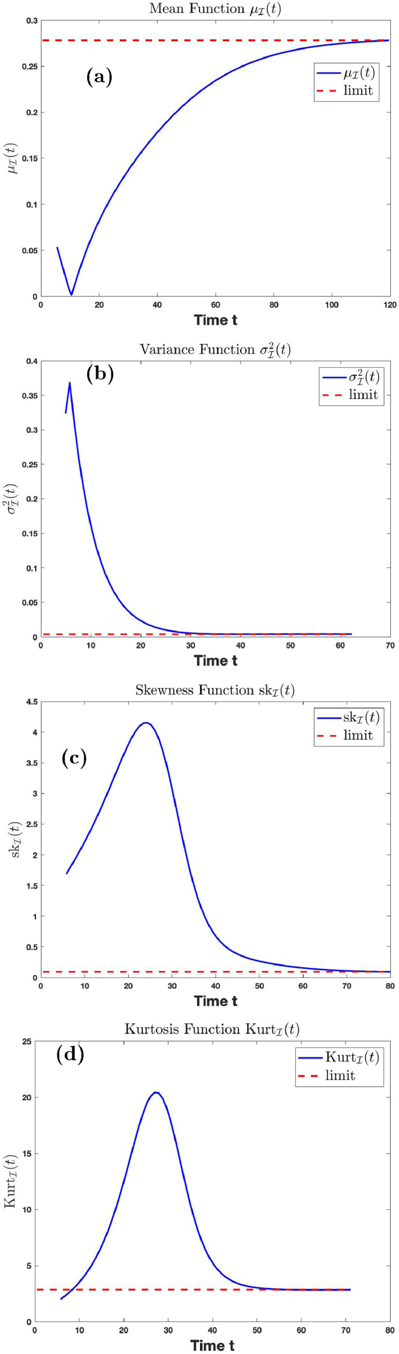
Fig. 2 (a), (b) and (c) is the graph of the probability density function $p_{\mathcal{I}}(\mathcal{I},t|{\mathcal{I}}_0=0.05)$ for the case where $\beta =0.5,$ $\beta =0.8,$ and $\beta =1,$ respectively. Here, we use $\mu =\frac{1}{80.3\times 365},$ $\gamma =1/7$ and $\sigma =0.65$. Fig. 2(d) shows the stationary probability distribution $p_{\mathcal{I}}^s\left(\mathcal{I}\right),$ which is the limiting distribution $\underset{t\to \infty }{lim}{p}_{\mathcal{I}}\left(\mathcal{I}\right|t,{\mathcal{I}}_0=0.05)$. We see here that the distributions for the three cases skewed left. This is evident in Figs. 9(b) and 10(b) as we can see there that the skewness plot is negative. We see from Fig. 2(d) that $p_{\mathcal{I}}\left(\mathcal{I}\right|t,{\mathcal{I}}_0=0.05)\to p_{\mathcal{I}}^s\left(\mathcal{I}\right)$ as $t\to \infty$. Also, we observe that as $\beta$ increases, the stationary density function shifts concentration to the right. The concentration moves closer to $I^{*}=\mathcal{N}=1$ as $\beta$ grows larger. This is because as the transmission rate increases, we expect the number of infection to increase until everyone in the population becomes infected. This can be confirmed analytically using (3.30).

Fig. 2.

Graphs of the probability density function $p_{\mathcal{I}}(\mathcal{I},t|{\mathcal{I}}_0=0.05)$ and $p_{\mathcal{I}}^s\left(\mathcal{I}\right)$ as $\beta$ increases.

Fig. 9.

Graphs of the mean, variance, skewness, kurtosis function with time.

Fig. 10.

Graphs of the mean, variance, skewness, kurtosis function with time.

4.1.3. Behavior of the distribution of $\mathcal{I}$ as $R_0\to 1^{+}$ and ${\mathcal{R}}_0\to 1^{+}$.

As shown in Theorem 1, the disease will die out on the long run if ${\mathcal{R}}_0\le 1$ (implying $R_0\le 1$ also). Fig. 3(a) and (b) show the behavior of the distribution as disease dies out in the population using parameters $\mu =\frac{1}{80.3\times 365},\gamma =1/7,$ $\sigma =0.1$ and varying $\beta$ so that $R_0\to 1^{+}$ in 3(a) and ${\mathcal{R}}_0\to 1^{+}$ in 3(b). The result shows that on the long run, the density function of $\mathcal{I}$ converges to the Dirac delta function $\delta \left(\mathcal{I}\right)$ as ${\mathcal{R}}_0\to 1^{+}$.

Fig. 3.

Stationary density function $p_{\mathcal{I}}(\mathcal{I},)$ for the case where $R_0\to 1^{+}$ and ${\mathcal{R}}_0\to 1^{+},$ respectively.

4.1.4. Effect of change in temporary recovery rate

It follows from condition (3.11) that $0<\gamma <\beta -\mu$.

Fig. 4 (a) and (b) shows the effect of increase in the parameter $\gamma$ on the stationary density function $p_{\mathcal{I}}^s\left(\mathcal{I}\right)$ using parameters $\mu =\frac{1}{80.3\times 365},$ $\beta =0.5,$ with $\sigma =0.1$ in Fig. 4(a), and $\sigma =0.3$ in Fig. 4(b), respectively. We see here that as $\gamma$ increases to $\beta -\mu$ from the left, the distribution shifts concentration to the left until it concentrates entirely on 0. This shows that the disease dies out as $\gamma \to \beta -\mu$. We also see the effect of large noise in the system as $\gamma$ increases. We see that the distribution becomes taller and narrower in the presence of small noise, and flatter and wider in the presence of large noise. In Fig. 4(c), we see that the stationary distribution $p_{\mathcal{I}}^s\left(\mathcal{I}\right)$ concentrates more on the final size of the epidemic as the recovery rate decreases to zero. This analysis shows that the disease dies out as the recovery rate $\gamma$ reaches the threshold $\beta -\mu$. The number of infected reaches maximum as the number of those who recovered declines to zero.

Fig. 4.

Effect of changing $\gamma$ on the stationary density function $p_{\mathcal{I}}^s\left(\mathcal{I}\right)$.

4.1.5. Distribution for the case where $\mathcal{A}\approx 0$.

Fig. 5 (a) and (b) show the probability and stationary density functions $p_{\mathcal{I}}\left(\mathcal{I}\right|t,{\mathcal{I}}_0=0.05)$ and $p_{\mathcal{I}}\left(\mathcal{I}\right),$ respectively, for the case where $\beta -(\mu +\gamma )-{\sigma }^2/2\approx 0,$ or equivalently, $\overline{\mathcal{A}}\approx 0$ using parameters in Table 1 with $\beta =0.5,$ $\sigma =0.65$. We see here that as $\mathcal{I}\to 1^{-},$ the stationary distribution $p_{\mathcal{I}}^s\left(\mathcal{I}\right)\to \infty$. This follows directly from (3.30).

Fig. 5.

Probability and stationary density functions $p_{\mathcal{I}}\left(\mathcal{I}\right|t,{\mathcal{I}}_0=0.05)$ and $p_{\mathcal{I}}^s\left(\mathcal{I}\right),$ respectively, for the case where $\overline{\mathcal{A}}\approx 0$.

4.1.6. Distribution for the case where $\mu +\gamma \approx 0$.

Fig. 6 shows the probability density function $p_{\mathcal{I}}\left(\mathcal{I}\right|t,{\mathcal{I}}_0=0.05)$ for the case where $E=\mu +\gamma =0$ using parameters in Table 1 with $\beta =0.5,$ $\sigma =0.7$. The analysis also shows that if the number of infection is not harvested in any way (in this case, by recovering), then $p_{\mathcal{I}}\left(\mathcal{I}\right|t,{\mathcal{I}}_0)\to \infty$ as $\mathcal{I}\to {\mathcal{N}}^{-}$ for some $T>0$ with $t<T$. Also, we see that $p_{\mathcal{I}}^s\left(\mathcal{I}\right)=0$. This is true because if $E=0,$ $p_{\mathcal{I}}\left(\mathcal{I}\right|t,{\mathcal{I}}_0)=\frac{\mathcal{N}}{\mathcal{I}(\mathcal{N}-\mathcal{I})\sigma \sqrt{2\pi t}}\exp (-\frac{{(\ln \left(\frac{\mathcal{I}}{(\mathcal{N}-\mathcal{I})}\frac{(\mathcal{N}-{\mathcal{I}}_0)}{{\mathcal{I}}_0}\right)-\beta t)}^2}{2t{\sigma }^2})\to 0$ if $0<\mathcal{I}<\mathcal{N}$ as t→∞

Fig. 6.

Probability density function $p_{\mathcal{I}}\left(\mathcal{I}\right|t,{\mathcal{I}}_0=0.05)$ for the case where $E=\mu +\gamma \approx 0$.

4.1.7. Effect of noise in the system

Fig. 7 shows the effect of noise intensity $\sigma$ on the stationary density function $p_{\mathcal{I}}^s\left(\mathcal{I}\right)$ using $\mu =\frac{1}{80.3\times 365},$ $\beta =0.5,$ $\gamma =1/7$ and varying $\sigma$. Fig. 7(a) shows the distribution as $\sigma \to 0$ while Fig. 7(b) shows the distribution as $\sigma \to \infty$. We see from Fig. 7(a) that the stationary density function concentrates entirely on the number $I^{*}=(1-\frac{1}{R_0})\mathcal{N}$ as $\sigma \to 0$. This is because the solution

$$\mathcal{I}\left(t\right)=\frac{(1-\frac{1}{R_0})\mathcal{N}}{1+\frac{(1-\frac{1}{R_0})\mathcal{N}-{\mathcal{I}}_0}{{\mathcal{I}}_0}{e}^{-(\beta -(\mu +\gamma \left)\right)t}}$$

of the deterministic equivalent of (3.4) where $\sigma =0$ converges to $I^{*}=(1-\frac{1}{R_0})\mathcal{N}$ if $R_0>1$. The number $I^{*}=(1-\frac{1}{R_0})\mathcal{N}$ is the endemic equilibrium of the deterministic equivalent of (3.4) where $\sigma =0$. Endemic persists in the deterministic system if $R_0>1$. This is confirmed in Fig. 7(a). The graph shows that $p_{\mathcal{I}}^s\left(\mathcal{I}\right)\to \delta (\mathcal{I}-I^{*}),$ the Dirac delta function, as $\sigma \to 0^{+}$. This is not the case for large $\sigma$. In fact, as $\sigma \to \infty ,$ the stationary density function $p_{\mathcal{I}}^s\left(\mathcal{I}\right)\to \infty$ as $\mathcal{I}\to 0^{+}$ and as $\mathcal{I}\to 1^{-}$.

Fig. 7.

Effect of noise intensity $\sigma$ on the stationary density function $p_{\mathcal{I}}^s\left(\mathcal{I}\right)$.

4.2. Plot of the mean, variance, skewness, and kurtosis function using published parameters

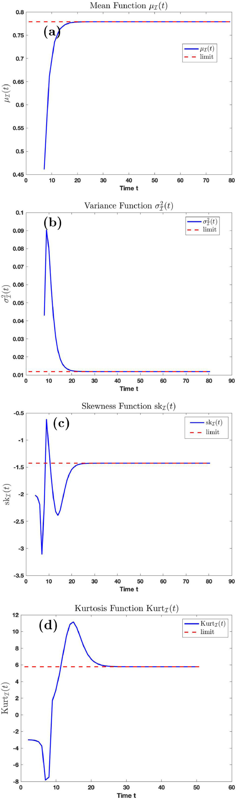
Fig. 8 (a), (b), (c) and (d) is the graph of the mean, variance, skewness, and kurtosis, respectively, of the distribution $p_{\mathcal{I}}\left(\mathcal{I}\right|t,{\mathcal{I}}_0=0.04)$ at time $t$ using parameters in Table 1 with $\mu =\frac{1}{80.3\times 365},$ $\beta =0.2,$ $\gamma =1/7$ and $\sigma =0.1$. The dashed line is the horizontal line representing the limits $\underset{t\to \infty }{lim}{\mu }_{\mathcal{I}}\left(t\right),$ $\underset{t\to \infty }{lim}{\sigma }_{\mathcal{I}}^2\left(t\right),$ $\underset{t\to \infty }{lim}{\text{sk}}_{\mathcal{I}}\left(t\right),$ $\underset{t\to \infty }{lim}{\text{Kurt}}_{\mathcal{I}}\left(t\right)$ of the mean, variance, skewness, and kurtosis functions, respectively, of the distribution $p_{\mathcal{I}}^s\left(\mathcal{I}\right),$ given in (3.40). Fig. 8(a) shows that if the transmission rate is $\beta =0.2$ and the temporary recovery rate is as low as $\gamma =1/7,$ the average number of infection cases will rise to $28\%$ on the long run if proper care and prevention is not taken. The variance function converges to 0.0039 on the long run. This shows the magnitude of the spread of the data away from the mean is small. The skewness function is a positive function, suggesting that the distribution of the data is skewed right.

Fig. 8.

Graphs of the mean, variance, skewness, kurtosis function with time.

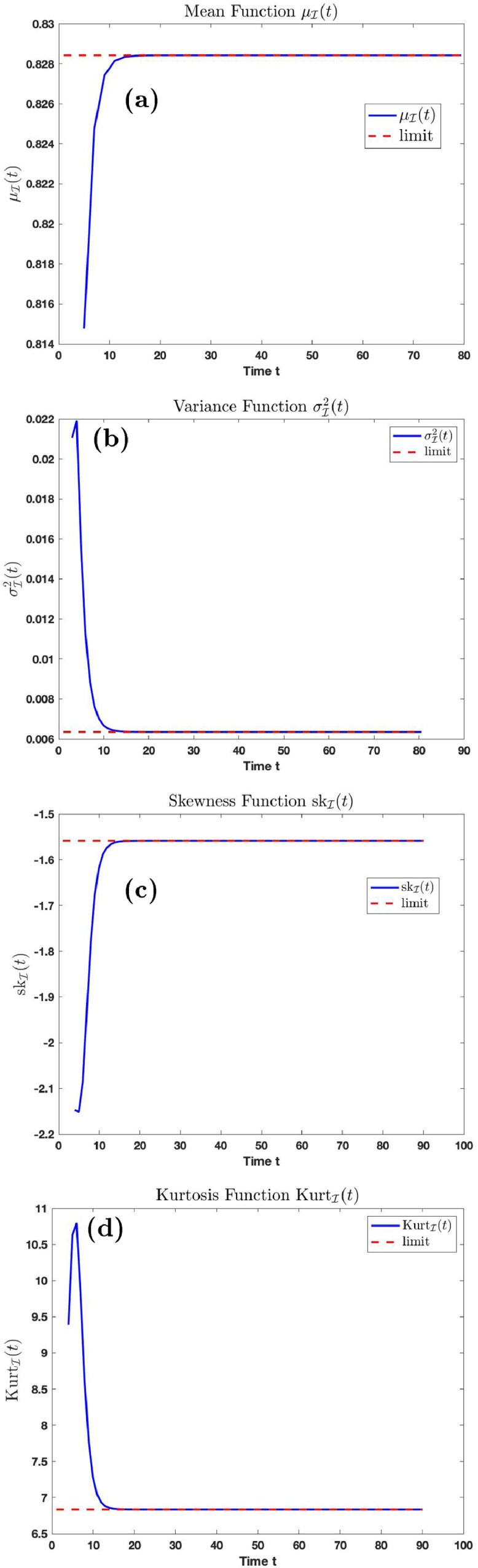
Fig. 9 (a), (b), (c) and (d) is the graph of the mean, variance, skewness, and kurtosis, respectively, of the distribution $p_{\mathcal{I}}\left(\mathcal{I}\right|t,{\mathcal{I}}_0=0.05)$ at time $t$ using parameters in Table 1 with $\mu =\frac{1}{80.3\times 365},$ $\beta =0.8,$ $\gamma =1/7$ and $\sigma =0.65$. The dashed line is as described in Fig. 8. Fig. 9(a) shows that if the transmission rate is $\beta =0.8$ and the temporary recovery rate is as low as $\gamma =1/7,$ the average number of infection cases will rise to $77.9\%$ on the long run if proper care and prevention is not taken. The variance function converges to 0.012 on the long run. The skewness function is a negative function, suggesting that the distribution is left skewed.

Fig. 10 (a), (b), (c) and (d) is the graph of the mean, variance, skewness, and kurtosis, respectively, of the distribution $p_{\mathcal{I}}\left(\mathcal{I}\right|t,{\mathcal{I}}_0=0.05)$ at time $t$ using parameters in Table 1 with $\mu =\frac{1}{80.3\times 365},$ $\beta =1,$ $\gamma =1/7$ and $\sigma =0.65$. The dashed line is as described in Fig. 8. Fig. 10(a) shows that if the transmission rate is $\beta =1$ and the temporary recovery rate is as low as $\gamma =1/7,$ the average number of infection cases will rise to $82.8\%$ on the long run if proper care and prevention is not taken. The variance function converges to 0.0064 on the long run. The skewness function is a negative function. By comparing the results derived in Figs. 9 and 10, it follows that the average number of cases increases and the variance decreases on the long run as the transmission rate increases.

4.3. Probability distribution of aggregate number of COVID-19 infections in the United States

Several epidemiological models [1], [10], [23], [38], [43], [44], [49], [51], [57] have been developed to study the transmission of the COVID-19 virus. As it is well known, the generalized logistic equation is widely used in interpreting the aggregate number of COVID-19 infection trajectories in several countries [49], [50], [57]. We see in our work that model (2.2) is a logistic differential equation. In the case of modeling the aggregate number of infected cases, $\beta$ is referred to as the aggregate infection growth rate, $\mathcal{N}$ is the aggregate infection carrying capacity, and $(\mu +\gamma )$ serves as the aggregate infection harvesting effort. In this section, we study the trajectory and the distribution of the aggregate counts of COVID-19 cases reported by the Centers for Disease Control and Prevention (CDC)5 for some states in the United States using model (2.6) and the time-dependent density function (3.30), respectively. We assume the aggregate number of infection follows the model (2.6), where $\mathcal{I}\left(t\right)$ in this case represents the aggregate infection cases at time $t$. The advantage of using model (2.6) over most models available in literature is that it considers presence of external perturbations/disturbances in the contact rate of the disease that can be caused by many factors such as pneumonia seasonality, mobility, testing rates, mask use per capital weather [27], social behavior, strain-specific factors [42], and public health intervention [34]. Also, in the presence of this noise, the harvesting function is not constant as widely assumed, but non-linear.

Figs. 11, 12, and 13 shows the plot of the aggregate infection counts of COVID-19 cases for the states and territories: AK, AR, AZ, CA, CO, CT, DC, DE, GA, GU, HI, IA, ID, IL, IN, KS, KY, LA, MD, ME, MI, MN, MO, MP, MS, MT, NC, ND, NE, NH, NJ, NM, NV, OH, OK, OR, PA, RI, SC, SD, TN, TX, UT, VA, VT, WI, WV, WY, in the United States for the period 01/22/2020 to 03/23/2021 using model (2.6), and the parameters in the model estimated for the deterministic version of the model case using the Non-linear Least Squares estimation scheme [15], [36]. We also estimated the initial point ${\mathcal{I}}_0$ for better fit.

Fig. 11.

Real and simulated aggregate counts of COVID-19 infection for the states and territories: AK, AR, AZ, CA, CO, CT, DC, DE, GA, GU, HI, IA, ID, IL, IN, KS in the United States.

Fig. 12.

Real and simulated aggregate counts of COVID-19 infection for the states and territories: KY, LA, MD, ME, MI, MN, MO, MP, MS, MT, NC, ND, NE, NH, NJ, NM in the United States.

Fig. 13.

Real and simulated aggregate counts of COVID-19 infection for the states and territories: NV, OH, OK, OR, PA, RI, SC, SD, TN, TX, UT, VA, VT, WI, WV, WY in the United States.

The parameter estimates $\widehat{\mathcal{N}},$ $\widehat{\beta },$ $\widehat{\gamma },$ and ${\widehat{\mathcal{I}}}_0$ of the aggregate infection carrying capacity $\mathcal{N},$ the infection growth rate $\beta ,$ the infection recovery rate $\gamma ,$ and the initial population size ${\mathcal{I}}_0$ are estimated along with the root mean square error (RMSE) of the estimation and reported in Table 2 . $T$ is the number of non-zero aggregate infection days from January 22, 2020 to March 23, 2021. The trajectory of the aggregate infection counts, together with the estimated trajectory for each of the 48 states and territories studied are reported in Fig. 11, Fig. 12, and 13. The red and blue curves are the trajectory for the real and simulated COVID-19 aggregate count data, respectively. The estimated parameter $\widehat{\mathcal{N}}$ here represents the carrying capacity of the aggregate infection count for each states. We show in later section that as the aggregate harvesting effort $\mu +\gamma$ reduces, or as the aggregate infection growth rate increases due to no proper public health intervention, the aggregate COVID-19 count estimate converges to $\widehat{\mathcal{N}}$.

Table 2.

Parameter estimates and the RMSE for the period of Jan 22, 2020-March 23, 2021.

State	$\widehat{\mathcal{N}}$	$\widehat{\beta }$	$\widehat{\gamma }$	${\mathcal{I}}_0$	$T$	RMSE
AK	116955	0.06495	0.03196	11.7	373	1169.2
AR	1387119	0.05572	0.03857	3073.4	374	8295.1
AZ	6207611	0.05191	0.03901	10109.9	419	42953.8
CA	18525258	0.04999	0.03442	18040.2	419	180570.9
CO	1287227	0.06487	0.04007	528.3	381	17744.6
CT	4265220	0.05993	0.04875	8086.5	377	16566.6
DC	1139045	0.06526	0.05747	3.501.3	379	1926.8
DE	993497	0.06256	0.05049	2217.8	375	3.887.0
GA	7996680	0.06166	0.04890	23805.8	386	38483.0
GU	14309	0.06804	0.03079	2.4421	371	152.2
HI	88343	0.066541	0.045843	$231.96$	381	1164.9
IA	1047217	0.058366	0.037049	$1664.8$	378	10774
ID	490785	0.055512	0.033361	$688.45$	372	4195.1
IL	4441504	0.053073	0.035285	$5387.3$	422	47364
IN	1783274	0.057553	0.033006	$898.27$	380	24196
KS	868640	0.058924	0.035784	$615.67$	378	7801
KY	1386548	0.06343	0.041157	$797.04$	379	7928.9
LA	3399215	0.063446	0.051774	19790	377	17743
MD	4032036	0.062989	$0.0521$	16646	381	15558
ME	152787	$0.0656$	0.040101	$24.428$	374	2044
MI	2316851	0.057358	0.037583	$3746.3$	376	32390
MN	1243941	0.061734	0.035266	$555.81$	380	20819
MO	1580962	0.056665	0.033793	$1439.2$	379	10266
MP	857	0.066576	0.053355	$10.391$	358	2.8125
MS	1939174	0.063662	0.049823	$7495.3$	374	9953.3
MT	188925	0.064356	0.029378	$14.373$	375	1290
NC	4994376	0.056624	0.041666	10277	384	26445
ND	174226	0.064338	0.026613	$14.732$	374	2473.8
NE	655227	0.062605	0.040601	$714.66$	380	7454
NH	232013	0.065474	0.038755	$24.024$	384	3291.7
NJ	21306864	0.064247	0.055493	45087	381	44812
NM	511161	0.062123	0.036503	$208.01$	375	7326.1
NV	1387057	0.065965	0.048652	$2906.5$	381	11652
OH	2680011	0.060963	0.035346	$871.78$	376	35223
OK	1386379	0.056107	0.035141	$1358.7$	379	10747
OR	655383	0.063132	0.043888	$674.69$	386	4765.3
PA	3720047	0.06246	0.041921	$2585.5$	380	44433
RI	559165	0.051781	0.035041	$975.64$	384	6601.1
SC	4294273	0.060356	0.047188	10037	381	20568
SD	245266	0.067793	0.035468	$43.639$	376	3069.5
TN	3173919	0.05427	0.036698	$6150.5$	381	26324
TX	17156629	0.05962	0.045363	43642	381	78597
UT	1095558	0.054204	0.03238	$1074.7$	378	9331.2
VA	5879402	0.056827	0.044575	13170	378	19814
VT	132684	0.076231	0.058152	$46.712$	378	607.51
WI	1372907	0.058849	0.030678	$477.69$	383	13913
WV	327686	0.064602	0.034811	36.89	369	3243.5
WY	99777	0.070869	0.031364	$2.2229$	374	1245.1

4.3.1. Distribution of the aggregate infection count in the United States for March 23, 2021

Here, we study the effect of small disturbances in the system by setting $\sigma =0.08$ and plot the distribution of the aggregate number of infection that occurred on March 23, 2021 for the state of AK, ID, KY, ND, SD, WI, WV, WY. Let $T$ be the number of non-zero days from January 22, 2020 (first day CDC started recording data) to March 23, 2021. We plot the curve for the distribution $p_{\mathcal{I}}\left(\mathcal{I}\right|t=T,{\widehat{\mathcal{I}}}_0),$ together with the density function obtained from the histogram of the random variable $\left\{{\mathcal{I}}_T^l\right\},$ $l=1,2,\cdots ,L,$ in (4.1) for $L=10,000$ simulations. The value of $T$ for each of the states analyzed are reported in Table 3 . We confirm the result derived in Fig. 7(a), that is, the probability density function $p_{\mathcal{I}}\left(\mathcal{I}\right|t=T,{\widehat{\mathcal{I}}}_0)$ of the aggregate count of COVID-19 for March 23, 2021 concentrates entirely on the number $\overline{\mathcal{N}}=(1-\frac{1}{R_0})\mathcal{N}$ for small $\sigma$. This result is shown in Fig. 14 . The analysis shows that the aggregate count of COVID-19 for the states analyzed converges to $\overline{\mathcal{N}}$ asymptotically on the day March 23, 2021. This number is estimated and reported in Table 3.

Table 3.

Parameter estimate $\overline{\mathcal{N}}$ for the day March 23, 2021.

State	AK	ID	KY	ND	SD	WI	WV	WY
$\overline{\mathcal{N}}$	59355	195541	486138	102066	116825	656407	150941	55572

Fig. 14.

Probability distribution of aggregate number of counts that occurred on March 23, 2021.

4.3.2. Distribution of the final size of the aggregate infection count in the United States

In this section, we study and analyze the distribution of the final size of the aggregate infection count in the United States by studying how the distribution $p_{\mathcal{I}}\left(\mathcal{I}\right|t,{\widehat{\mathcal{I}}}_0)$ behaves as $t\to \infty$. According to (3.34), we know that

$$\underset{t\to \infty }{lim}{p}_{\mathcal{I}}\left(\mathcal{I}\right|t,{\widehat{\mathcal{I}}}_0)=p_{\mathcal{I}}^s\left(\mathcal{I}\right).$$

We verify this by plotting, for large $t,$ say, $t=100,000,$ the distribution $p_{\mathcal{I}}\left(\mathcal{I}\right|t,{\widehat{\mathcal{I}}}_0)$ together with $p_{\mathcal{I}}^s\left(\mathcal{I}\right)$. The verification plot is shown in Fig. 15 . For this reason, we analyze the distribution of the final size of the aggregate infection count using the stationary probability density function $p_{\mathcal{I}}^s\left(\mathcal{I}\right)$.

Fig. 15.

Comparison of the probability density function $p_{\mathcal{I}}^s\left(\mathcal{I}\right)$ and $\underset{t\to \infty }{lim}{p}_{\mathcal{I}}\left(\mathcal{I}\right|t,{\mathcal{I}}_0)$.

Fig. 15 shows the comparison of the stationary density function $p_{\mathcal{I}}^s\left(\mathcal{I}\right)$ (in red color) and the limiting distribution $\underset{t\to \infty }{lim}{p}_{\mathcal{I}}\left(\mathcal{I}\right|t,{\mathcal{I}}_0)$ (in blue color).

As evidenced in Fig. 2(d), we see that the stationary probability density function $p_{\mathcal{I}}^s\left(\mathcal{I}\right)$ concentrates more on the final size of the epidemic $\widehat{\mathcal{N}}$ as the infection growth rate $\beta$ increases. We also see a similar behavior in Figs. 4(c) and 7 (b) as the aggregate harvesting effort $\mu +\gamma$ reduces and as the noise intensity $\sigma$ increases, respectively. For this reason, we study the effect of high infection growth rate $\beta ,$ low recovery rate (low aggregate harvesting effort $\mu +\gamma$), and effect of large noise on the distribution of the aggregate COVID-19 counts in the United States in the following subsections. This is done by plotting the stationary probability density function $p_{\mathcal{I}}^s\left(\mathcal{I}\right)$ of the final size of the aggregate infection count for large, small, and large $\beta ,$ $\gamma$, and $\sigma ,$ respectively. We see that the graph of $p_{\mathcal{I}}^s\left(\mathcal{I}\right)$ concentrates on the estimate $\widehat{\mathcal{N}}$ (obtained in Table 2), which is the aggregate carrying capacity of the COVID-19 count in the United States as public health intervention reduced.

Fig. 16 shows the distribution of the final size of the aggregate infection count as the infection growth rate $\beta$ increases using the estimated parameters in Table 2 with large noise intensity $\sigma =0.2$ and varying infection growth rates $\beta =0.06$ (blue curve), $\beta =0.15$ (black curve), and $\beta =0.3$ (red curve) for each states analyzed. The figure shows that if proper intervention is not taken (resulting in increase in infection growth rate $\beta$ and constant recovery rate $\gamma$), the aggregate count of COVID-19 infection will rise to the estimated aggregate carrying capacity value $\widehat{\mathcal{N}}$ in Table 2 for each respective states and territories. The analysis was done for the 48 states and territories mentioned in Table 2 and similar results obtained for each states and territories. For this reason and in order to minimize space, we only report the plots for the state of AK, ID, KY, ND, SD, WI, WV, WY.

Fig. 16.

Distribution $p_{\mathcal{I}}^s\left(\mathcal{I}\right)$ of the final size of the aggregate infection as the infection growth rate $\beta$ increases for the states: AK, ID, KY, ND, SD, WI, WV, WY in the United States.

Fig. 17 shows the distribution of the final size of the aggregate infection count as the aggregate harvesting effort decreases using the estimated parameters in Table 2 with large noise intensity $\sigma =0.2$ and varying recovery rate $\gamma =0.02$ (blue curve), $\gamma =0.015$ (black curve), and $\gamma =0.01$ (red curve) for each states analyzed. The figure shows that if proper intervention is not taken (resulting in decline in recovery rate $\gamma$ and constant aggregate growth rate $\beta$), the aggregate count of COVID-19 infection will rise to the estimated aggregate carrying capacity value $\widehat{\mathcal{N}}$ in Table 2 for each respective states and territories. The analysis was done for the 48 states and territories mentioned in Table 2 and similar results obtained for each states and territories. We only report the plots for the state of AK, ID, KY, ND, SD, WI, WV, WY here.

Fig. 17.

Distribution $p_{\mathcal{I}}^s\left(\mathcal{I}\right)$ of the final size of the aggregate infection as the aggregate harvesting rate $\mu +\gamma$ reduces with large noise $\sigma$ for the states: AK, ID, KY, ND, SD, WI, WV, WY in the United States.

5. Results, conclusion and discussion

By assuming the contact rate $\mathit{\beta }$ of certain diseases is affected by environmental perturbations, we convert the general deterministic SIS epidemic model with vital dynamics and constant population to a stochastic SIS model and used this model to study the dynamics of some infectious diseases. The study in this work involves analyzing the distribution of numbers of infections whose dynamic follows the SIS stochastic model (2.6). To do this, we derive the closed-form time-dependent probability density function $p_{\mathcal{I}}\left(\mathcal{I}\right|t,{\mathcal{I}}_0)$ of the number of infection $\mathcal{I}$ at time $t$ given the initial point ${\mathcal{I}}_0$. The stationary probability density function $p_{\mathcal{I}}^s\left(\mathcal{I}\right)$ of the process is also derived and analyzed and our studies show that $p_{\mathcal{I}}\left(\mathcal{I}\right|t,{\mathcal{I}}_0)$ converges to $p_{\mathcal{I}}^s\left(\mathcal{I}\right)$ on the long run. We showed that these distibutions exist if the average number, $R_0,$ of individuals infected by an infectious individual in a completely susceptible population is more than one. Also, we showed that the disease will die out if $R_0\le 1$. Using the Milstein scheme, the stochastic model (2.6) is discretized for $N$ sample size and $L$ simulations and the correctness of the obtained probability density functions $p_{\mathcal{I}}\left(\mathcal{I}\right|t=2,{\mathcal{I}}_0)$ and $p_{\mathcal{I}}^s\left(\mathcal{I}\right)$ are verified in Section 4.1.1 by comparing them to the probability density function derived from the histogram of the discretized processes ${\mathcal{I}}_{20}^l$ and ${\mathcal{I}}_N^l$ (for large $N$), respectively, in (4.1), for $1\le j\le N,$ $1\le l\le L,$ and $\Delta t=1/10$ using published epidemiological data. The effect of changes in the transmission rate and temporary recovery rate on the distribution $p_{\mathcal{I}}\left(\mathcal{I}\right|t,{\mathcal{I}}_0)$ and $p_{\mathcal{I}}^s\left(\mathcal{I}\right)$ is studied. It was shown that as $R_0$ approaches 1 (from above), the distribution $p_{\mathcal{I}}^s\left(\mathcal{I}\right)$ approaches the Dirac delta function $\delta \left(\mathcal{I}\right)$ and concentrates entirely on zero. That is, on the long run, the number of infection declines and the disease eventually dies out as the reproduction number $R_0$ approaches 1 (from above). Also, as the recovery rate decreases to zero, the distribution of the number of infection shifts concentration to the right until it concentrates entirely on the infection carrying capacity $\mathcal{N}$. That is, the infected population converges to the infection carrying capacity $\mathcal{N}$ as the recovery rate reduces significantly. A similar analysis done on the transmission rate $\beta$ shows that the infected population converges to the infection carrying capacity $\mathcal{N}$ as $\beta$ increases. The effect of noise on the system is also analyzed. It was shown that on the long run, the probability density function $p_{\mathcal{I}}\left(\mathcal{I}\right|t,{\mathcal{I}}_0)$ shifts concentration on the disease endemic equilibrium point $(1-\frac{1}{R_0})\mathcal{N}$ as the noise intensity $\sigma$ approaches zero. This is because (2.2) has an endemic equilibrium $(1-\frac{1}{R_0})\mathcal{N}$ that is globally stable if $R_0>1$. Some properties of the time-dependent probability density function, namely the mean, variance, skewness, and Kurtosis functions are derived and analyzed as a function of time.

Similar analysis described above is done using the real aggregate counts of COVID-19 cases reported by the Centers for Disease Control and Prevention for the states: AK, AR, AZ, CA, CO, CT, DC, DE, GA, GU, HI, IA, ID, IL, IN, KS, KY, LA, MD, ME, MI, MN, MO, MP, MS, MT, NC, ND, NE, NH, NJ, NM, NV, OH, OK, OR, PA, RI, SC, SD, TN, TX, UT, VA, VT, WI, WV, WY in the United States. We study the trajectory and the distribution of the aggregate counts using the time-dependent density function $p_{\mathcal{I}}\left(\mathcal{I}\right|t,{\mathcal{I}}_0)$ and stationary distribution $p_{\mathcal{I}}^s\left(\mathcal{I}\right)$ given in (3.30). The validity of the derived time-dependent density function $p_{\mathcal{I}}\left(\mathcal{I}\right|t,{\mathcal{I}}_0)$ is verified by comparing the distribution $p_{\mathcal{I}}\left(\mathcal{I}\right|t=T,{\mathcal{I}}_0)$ for the aggregate count of COVID-19 for the day March 23, 2021 with the histogram of the distribution of the random variable ${\mathcal{I}}_T^l,$ $l=1,2,\cdots ,L,$ for $L=10,000$ simulations, where $T$ is the number of non-zero days from January 1, 2020 to March 23, 2021. We also show numerically using the real COVID-19 aggregate counts for AK, ID, KY, ND, SD, WI, WV, WY that on the long run, the time-dependent density function $p_{\mathcal{I}}\left(\mathcal{I}\right|t,{\mathcal{I}}_0)$ converges to the stationary density function $p_{\mathcal{I}}^s\left(\mathcal{I}\right)$. We use the distribution to confirm the estimate of the aggregate count for the month of March 23, 2021 in Table 3 and compare the result with the real data. By studying the distribution of the final size of the aggregate infection counts, our analysis shows that on the long run, if proper intervention is not taken such that the harvesting effort decreases significantly to 0.01 (or less), the aggregate counts of COVID-19 cases for each states may increase to the value $\widehat{\mathcal{N}}$ reported in Table 2. A similar analysis shows that the aggregate counts of COVID-19 cases for each states may increase to the value $\widehat{\mathcal{N}}$ if the infection growth rate increases to 0.3 (or more). These studies are confirmed by showing that the distribution $p_{\mathcal{I}}^s\left(\mathcal{I}\right)$ shifts concentration on the value $\widehat{\mathcal{N}}$ as the harvesting effort decreases or the infection growth rate increases. More studies are still ongoing on the distribution of the aggregate count of infection as data are being updated daily. Further extension of the result obtained in this work using fractional order cases as discussed in Jajarmi et al. [28], [29] is under investigation. For more readings on fractional derivatives, we direct readers to the papers [3], [4], [51], [56].

Availability of data and materials

The data used in the analysis can be found on the CDC${}^5$ website.

Funding

This research did not receive any specific grant from funding agencies in the public, commercial, or not-for-profit sectors.

CRediT authorship contribution statement

Olusegun Michael Otunuga: Conceptualization, Data curation, Formal analysis, Software, Writing - original draft, Writing - review & editing.

Declaration of Competing Interest

The author declares that there is no known competing financial interests or personal relationships that could have appeared to influence the work reported in this paper.

Appendix A. Supplementary materials

Supplementary Data S1

Supplementary Raw Research Data. This is open data under the CC BY license http://creativecommons.org/licenses/by/4.0/

Supplementary Data S2

Supplementary Raw Research Data. This is open data under the CC BY license http://creativecommons.org/licenses/by/4.0/

Supplementary Data S3

Supplementary Raw Research Data. This is open data under the CC BY license http://creativecommons.org/licenses/by/4.0/

Supplementary Data S4

Supplementary Raw Research Data. This is open data under the CC BY license http://creativecommons.org/licenses/by/4.0/

Supplementary Data S5

Supplementary Raw Research Data. This is open data under the CC BY license http://creativecommons.org/licenses/by/4.0/

Supplementary Data S6

Supplementary Raw Research Data. This is open data under the CC BY license http://creativecommons.org/licenses/by/4.0/

Supplementary Data S7

Supplementary Raw Research Data. This is open data under the CC BY license http://creativecommons.org/licenses/by/4.0/

Supplementary Data S8

Supplementary Raw Research Data. This is open data under the CC BY license http://creativecommons.org/licenses/by/4.0/

Supplementary Data S9

Supplementary Raw Research Data. This is open data under the CC BY license http://creativecommons.org/licenses/by/4.0/

Supplementary Data S10

Supplementary Raw Research Data. This is open data under the CC BY license http://creativecommons.org/licenses/by/4.0/

Supplementary Data S11

Supplementary Raw Research Data. This is open data under the CC BY license http://creativecommons.org/licenses/by/4.0/

Supplementary Data S12

Supplementary Raw Research Data. This is open data under the CC BY license http://creativecommons.org/licenses/by/4.0/

Supplementary Data S13

Supplementary Raw Research Data. This is open data under the CC BY license http://creativecommons.org/licenses/by/4.0/

Supplementary Data S14

Supplementary Raw Research Data. This is open data under the CC BY license http://creativecommons.org/licenses/by/4.0/

Supplementary Data S15

Supplementary Raw Research Data. This is open data under the CC BY license http://creativecommons.org/licenses/by/4.0/

Supplementary Data S16

Supplementary Raw Research Data. This is open data under the CC BY license http://creativecommons.org/licenses/by/4.0/

Supplementary Data S17

Supplementary Raw Research Data. This is open data under the CC BY license http://creativecommons.org/licenses/by/4.0/

Supplementary Data S18

Supplementary Raw Research Data. This is open data under the CC BY license http://creativecommons.org/licenses/by/4.0/

Supplementary Data S19

Supplementary Raw Research Data. This is open data under the CC BY license http://creativecommons.org/licenses/by/4.0/

Supplementary Data S20

Supplementary Raw Research Data. This is open data under the CC BY license http://creativecommons.org/licenses/by/4.0/

Supplementary Data S21

Supplementary Raw Research Data. This is open data under the CC BY license http://creativecommons.org/licenses/by/4.0/

Supplementary Data S22

Supplementary Raw Research Data. This is open data under the CC BY license http://creativecommons.org/licenses/by/4.0/

Supplementary Data S23

Supplementary Raw Research Data. This is open data under the CC BY license http://creativecommons.org/licenses/by/4.0/

Supplementary Data S24

Supplementary Raw Research Data. This is open data under the CC BY license http://creativecommons.org/licenses/by/4.0/

Supplementary Data S25

Supplementary Raw Research Data. This is open data under the CC BY license http://creativecommons.org/licenses/by/4.0/

Supplementary Data S26

Supplementary Raw Research Data. This is open data under the CC BY license http://creativecommons.org/licenses/by/4.0/

Supplementary Data S27

Supplementary Raw Research Data. This is open data under the CC BY license http://creativecommons.org/licenses/by/4.0/

Supplementary Data S28

Supplementary Raw Research Data. This is open data under the CC BY license http://creativecommons.org/licenses/by/4.0/

Supplementary Data S29

Supplementary Raw Research Data. This is open data under the CC BY license http://creativecommons.org/licenses/by/4.0/

Supplementary Data S30

Supplementary Raw Research Data. This is open data under the CC BY license http://creativecommons.org/licenses/by/4.0/

Supplementary Data S31

Supplementary Raw Research Data. This is open data under the CC BY license http://creativecommons.org/licenses/by/4.0/

Supplementary Data S32

Supplementary Raw Research Data. This is open data under the CC BY license http://creativecommons.org/licenses/by/4.0/

Supplementary Data S33

Supplementary Raw Research Data. This is open data under the CC BY license http://creativecommons.org/licenses/by/4.0/

Supplementary Data S34

Supplementary Raw Research Data. This is open data under the CC BY license http://creativecommons.org/licenses/by/4.0/

Supplementary Data S35

Supplementary Raw Research Data. This is open data under the CC BY license http://creativecommons.org/licenses/by/4.0/

Supplementary Data S36

Supplementary Raw Research Data. This is open data under the CC BY license http://creativecommons.org/licenses/by/4.0/

Supplementary Data S37

Supplementary Raw Research Data. This is open data under the CC BY license http://creativecommons.org/licenses/by/4.0/

Supplementary Data S38

Supplementary Raw Research Data. This is open data under the CC BY license http://creativecommons.org/licenses/by/4.0/

References

- 1.Abdullah S.A., Owyed S., Abdel-Aty A.-H., Mahmoud E.E., Shah K., Alrabaiah H. Mathematical analysis of COVID-19 via new mathematical model. Chaos Solitons Fractals. 2021;143:110585. doi: 10.1016/j.chaos.2020.110585. [DOI] [PMC free article] [PubMed] [Google Scholar]
- 2.Arnold L. Wiley; New York: 1974. Stochastic differential equations: theory and applications. [Google Scholar]
- 3.Baleanu D., Ghanbari B., Asad J.H., Jajarmi A., Pirouz H.M. Planar system-masses in an equilateral triangle: numerical study within fractional calculus. Comput Model Eng Sci. 2020;124(3):953–968. doi: 10.32604/cmes.2020.010236. [DOI] [Google Scholar]
- 4.Baleanu D., Jajarmi A., Sajjadi S.S., Asad J.H. The fractional features of a harmonic oscillator with position-dependent mass. Commun Theor Phys. 2020;72(5):055002. [Google Scholar]
- 5.Bateman H. Vols. 1 & 2. McGraw-Hill; New York: 1953. Higher transcendental functions. [Google Scholar]
- 6.Becker P. Infinite integrals of Whittaker and Bessel functions with respect to their index. Math Phys. 2009;50:123515. [Google Scholar]
- 7.Beddington J.R., May R.M. Harvesting natural populations in a randomly fluctuating environment. Science. 1977;197:463–465. doi: 10.1126/science.197.4302.463. [DOI] [PubMed] [Google Scholar]
- 8.Bhatt N., Bhattacharyya S. Time evolution of the probability density function of a gamma-ray burst: a possible indication of the turbulent origin of gamma-ray bursts. MonNotRAstronSoc. 2012;420:1706–1713. [Google Scholar]
- 9.Carney M., Cunningham P., Byrne S. The benefits of using a complete probability distribution when decision making: an example in anticoagulant drug therapy. Med Decis Making. 2005 [Google Scholar]
- 10.Brahim Boukanjime B., Caraballo T., Fatini M.E., Khalifia M.E. Dynamics of a stochastic coronavirus (COVID-19) epidemic model with Markovian switching. Chaos Solitons Fractals. 2020;141:110361. doi: 10.1016/j.chaos.2020.110361. [DOI] [PMC free article] [PubMed] [Google Scholar]
- 11.Brauer F., Allen L.J.S., van den D., Wu J. Mathematical epidemiology lecture notes in mathematics. Math Biosci Subseries. 2008:1945. [Google Scholar]
- 12.Caughey T.K., Dienes J.K. Analysis of a nonlinear first-order system with a white noise input. J Appl Phys. 1961;32:2476–2479. [Google Scholar]
- 13.Caughey T.K. Nonlinear theory of random vibrations. Adv Appl Mech. 1971;11:209–253. [Google Scholar]
- 14.Caughey T.K. On the response of non-linear oscillator to stochastic excitation. Prob Eng Mech. 1986;1:2–4. [Google Scholar]
- 15.Coleman T.F., Li Y. An interior, trust region approach for nonlinear minimization subject to bounds. SIAM J Optim. 1996;6:418–445. [Google Scholar]
- 16.Dalal N., Greenhalgh D., Mao X. A stochastic model of AIDS and condom use. J Math Anal Appl. 2007;325:36–53. [Google Scholar]
- 17.Paola M.D., Ricciardi G., Vasta M. A method for the probabilistic analysis of non-linear systems. Prob Eng Mech. 1995;10:1–10. [Google Scholar]
- 18.Eikenberry S.E., Mancuso M., Iboi E., Phan T., Eikenberry K., Kuang Y., Kostelich E., Gumel A.B. To mask or not to mask: modeling the potential for face mask use by the general public to curtail the COVID-19 pandemic. Infect. Dis. Modell. 2020;5:293–308. doi: 10.1016/j.idm.2020.04.001. [DOI] [PMC free article] [PubMed] [Google Scholar]
- 19.Bogachev V.I., Krylov N.V., Rockner M., Shaposhnikov S.V. Fokker–Planck–Kolmogorov equations. Math Surv Monogr. 2015:207. [Google Scholar]
- 20.Gaines J.G., Lyons T.J. Random generation of stochastic area integrals. SIAM J Appl Math. 1994;54(4):1132–1146. [Google Scholar]
- 21.Gardiner C.W.. Handbook of stochastic methods for physics, chemistry and the natural sciences. 1985. New York, Springer-Verlag
- 22.Gray A., Greenhalgh D., Hu L., Mao X., Pan J. A stochastic differential equation SIS epidemic model. SIAM J Appl Math. 2011;71(3):876–902. [Google Scholar]
- 23.Habenom H., Suthar D.L., Purohit S.D. A numerical simulation on the effect of vaccination and treatments for the fractional hepatitis b model. J Comput Nonlin Dyn. 2021;16(1) [Google Scholar]
- 24.Heyde C.C., Hall P. Academic Press; New York London Toronto: 1980. large number theorem for martingales. [DOI] [Google Scholar]
- 25.Hethcote H.W., Yorke J.A. Lecture notes in biomathematics 1994; 56. Springer-Verlag; 1994. Gonorrhea transmission dynamics and control. [Google Scholar]
- 26.Holubec V., Kroy K., Steffenoni S. Physically consistent numerical solver for time-dependent Fokker–Planck equations. Phys Rev E. 2019;99:032117. doi: 10.1103/PhysRevE.99.032117. [DOI] [PubMed] [Google Scholar]
- 27.Team I.C.-. F.. Modeling COVID-19 scenarios for the United States. 2020. 10.1101/2020.10.08.20209510,
- 28.Jajarmi A., Baleanu D. On the fractional optimal control problems with a general derivative operator. Asian J Control. 2021;23(2):1062–1071. [Google Scholar]
- 29.Jajarmi A., Baleanu D. A new iterative method for the numerical solution of high-order non-linear fractional boundary value problems. Front Phys. 2020;8:220. doi: 10.3389/fphy.2020.00220. [DOI] [Google Scholar]
- 30.Jacquet Q., Kim E.-j., Hollerbach R. Time-dependent probability density functions and attractor structure in self-organised shear flows. Entropy. 2018;20:613. doi: 10.3390/e20080613. [DOI] [PMC free article] [PubMed] [Google Scholar]
- 31.Jin X., Wang Y., Huang Z., Paola M.D. Constructing transient response probability density of non-linear system through complex fractional moments. Int J Non-Linear Mech. 2014;65:253–259. [Google Scholar]
- 32.Johnson N.L., Scott R.A. Extension of eigenfunction-expansion solutions of a Fokker-Planck equation-II. second order system. Int J Non-Lin Mech. 1980;15(1):41–56. [Google Scholar]; 1980
- 33.Lajmanovich A., Yorke J.A. A deterministic model for gonorrhea in a nonhomogeneous population. Math Biosci. 1976;28:221–236. [Google Scholar]
- 34.Linka K., Peirlinck M., Kuhl E. The reproduction number of COVID-19 and its correlation with public health interventions. Computational Mechanics. 2020;66:1035–1050. doi: 10.1007/s00466-020-01880-8. [DOI] [PMC free article] [PubMed] [Google Scholar]
- 35.Lin Y.K., Cai G.Q. Advanced theory and applications. McGraw-Hill; New York: 1995. Probabilistic structural dynamics. [Google Scholar]
- 36.May R.M. An algorithm for least-squares estimation of nonlinear parameters. SIAM J Appl Math. 1963;11(2):431–441. [Google Scholar]
- 37.May R.M. 2nd ed. N.J. Princeton Univ. Press; Princeton: 1975. Stability and complexity in model ecosystems. [Google Scholar]
- 38.Memon Z., Qureshi S., Memon B.R. Assessing the role of quarantine and isolation as control strategies for COVID-19 outbreak: a case study. Chaos Solitons Fractals. 2021;144 doi: 10.1016/j.chaos.2021.110655. [DOI] [PMC free article] [PubMed] [Google Scholar]
- 39.Méndez V., Campos D., Horsthemke W. Stochastic fluctuations of the transmission rate in the susceptible-infected-susceptible epidemic model. Phys Rev E. 2012;86:011919. doi: 10.1103/PhysRevE.86.011919. [DOI] [PubMed] [Google Scholar]
- 40.Muscolino G. Dynamic motion: chaotic and stochastic behaviour. Springer; Vienna: 1993. Response of linear and non-linear structural systems under gaussian and non-Gaussian filtered input. (International Centre for Mechanical Sciences (Courses and Lectures), vol. 340). [Google Scholar]
- 41.Muscolino G., Ricciardi G., Vasta M. Stationary and non-stationary probability density function for non-linear oscillators. J Non-Lin Mech. 1997;32(6):1051–1064. [Google Scholar]
- 42.Mummert A., Otunuga O.M. Parameter identification for a stochastic SEIRS epidemic model: case study influenza. J Math Biol. 2019;79(2):705–729. doi: 10.1007/s00285-019-01374-z. [DOI] [PMC free article] [PubMed] [Google Scholar]
- 43.Naik P.A., Yavuz M., Qureshi S., Zu J. Modeling and analysis of COVID-19 epidemics with treatment in fractional derivatives using real data from Pakistan. Eur Phys J Plus. 2020;135(10):1–42. doi: 10.1140/epjp/s13360-020-00819-5. [DOI] [PMC free article] [PubMed] [Google Scholar]
- 44.Ndairou F., Area I., Nieto J.J., Torres F.M. Mathematical modeling of COVID-19 transmission dynamics with a case study of Wuhan. Chaos Solitons Fractals. 2020;135:109846. doi: 10.1016/j.chaos.2020.109846. [DOI] [PMC free article] [PubMed] [Google Scholar]
- 45.Nold A. Heterogeneity in disease transmission modelling. Math Biosci. 1980;52:227–240. [Google Scholar]
- 46.Olver F.W., Lozier D.W., Boisvert R.F., Clark C.W. National Institute of Sciences and Technology, U.S. Department of Commerce and Combridge University Press; Dubai, Tokyo and New York U.S.A.: 2010. NIST handbook of mathematical functions. [Google Scholar]
- 47.Otunuga O.M. Global stability for a dimensional HIV/AIDS epidemic model with treatments. Math Biosci. 2018;299:138–152. doi: 10.1016/j.mbs.2018.03.013. [DOI] [PubMed] [Google Scholar]
- 48.Otunuga O.M. Closed-form probability distribution of number of infections at a given time in a stochastic SIS epidemic model. Heliyon. 2019;5(9) doi: 10.1016/j.heliyon.2019.e02499. [DOI] [PMC free article] [PubMed] [Google Scholar]
- 49.Pelinovsky E., Kurkin A., Kurkina O., Kokoulina M., Epifanova A. Logistic equation and COVID-19. Chaos Solitons Fractals. 2020;140:110241. doi: 10.1016/j.chaos.2020.110241. [DOI] [PMC free article] [PubMed] [Google Scholar]
- 50.Pella J.S., Tomlinson P.K. A generalised stock-production model. Bull Inter-Am Trop Tuna Comm. 1969;13:421–496. [Google Scholar]
- 51.Peter O.J., Shaikh A.S., Ibrahim M.O., Nisar K.S., Baleanu D., Khan I., l e.a. Analysis and dynamics of fractional order mathematical model of COVID-19 in Nigeria using Atangana-Baleanu operator. Comput Mater Continua. 2021;66(2):1823–1848. [Google Scholar]
- 52.Szmytkowski R., Bielski S. An orthogonality relation for the Whittaker functions of the second kind of imaginary order. Integr Transforms Special Funct. 2010;21(10):739–744. [Google Scholar]
- 53.Roberts J.B., Spanos P.D. Wiley; New York: 1990. Random vibration and statistical linearization. [Google Scholar]
- 54.Sajjadi S.S., Baleanu D., Jajarmi A., Pirouz H.M. A new adaptive synchronization and hyperchaos control of a biological snap oscillator. Chaos Solitons Fractals. 2020;138:109919. [Google Scholar]
- 55.Tenké L.-M., Hollerbach R., Kim E.-j. Time-dependent probability density functions and information geometry in stochastic logistic and Gompertz models. J Stat Mech. 2017;2017:123201. [Google Scholar]
- 56.Tuan N.H., Tri V.V., Baleanu D. Analysis of the fractional corona virus pandemic via deterministic modeling. Math Meth Appl Sci. 2021;44(1):1086–1102. [Google Scholar]
- 57.Wang P., Zheng X., Li J., Zhu B. Prediction of epidemic trends in COVID-19 with logistic model and machine learning technics. Chaos Solitons Fractals. 2020;139:110058. doi: 10.1016/j.chaos.2020.110058. [DOI] [PMC free article] [PubMed] [Google Scholar]
- 58.Wijker J. Random vibrations in spacecraft structures design. Springer; Dordrecht: 2009. Fokker–Planck–Kolmogorov method or diffusion equation method. (Solid Mechanics and Its Applications, vol. 165). [Google Scholar]
- 59.Zhang X.-B., Chang S., Shi Q., Huo H.-F. Qualitative study of a stochastic SIS epidemic model with vertical transmission. Physica A. 2018;505:805–817. [Google Scholar]
- 60.Zhang X., Pandey M.D., Zhao Y. Probability density function for stochastic response of non-linear oscillation system under random excitation. Int J Non-Linear Mech. 2010;45(8):800–808. [Google Scholar]
Associated Data
This section collects any data citations, data availability statements, or supplementary materials included in this article.
Supplementary Materials