Refined Locally Linear Transform-Based Spectral-Domain Gradient Sparsity and Its Applications in Spectral CT Reconstruction

Abstract

Spectral computed tomography (CT) is extension of the conventional single spectral CT (SSCT) along the energy dimension, which achieves superior energy resolution and material distinguishability. However, for the state-of-the-art photon counting detector (PCD) based spectral CT, because the emitted photons with a fixed total number for each X-ray beam are divided into several energy bins, the noise level is increased in each reconstructed channel image, and it further leads to an inaccurate material decomposition. To improve the reconstructed image quality and decomposition accuracy, in this work, we first employ a refined locally linear transform to convert the structural similarity among two-dimensional (2D) spectral CT images to a spectral-dimension gradient sparsity. By combining the gradient sparsity in the spatial domain, a global three-dimensional (3D) gradient sparsity is constructed, then measured with L₁-, L₀- and trace-norm, respectively. For each sparsity measurement, we propose the corresponding optimization model, develop the iterative algorithm, and verify the effectiveness and superiority with real datasets.

I. INTRODUCTION

X-ray computed tomography (CT), as a nondestructive inspection technique, has been widely used in many fields, such as medicine, industry, biology, exploration, security, and so on [1]–[3]. Although the specific equipment design, scan protocol, and utilization purpose are greatly diverse, the fundamental image-forming principle is consistently based on the Beer–Lambert law, which describes the relation between X-ray and the object as an exponential attenuation model,

$$I\left(E\right)=I_0\left(E\right)\text{exp}\left(-\mathcal{P}\left(\mu \left(E,x\right)\right)\right),$$ (1)

where µ(E, x) is the linear attenuation coefficient for energy E at the position x [4], $\mathcal{P}(\cdot )$ a line integral operator (the ray transform and especially the Radon transform for 2D cases [5]), I₀(E) the emitted photons, and I(E) the collected photons. Actually, the validity of (1) is confined to a set of ideal imaging conditions, such as the X-ray energy is monochromatic, there is no scattering in the imaging process, and so on. However, in practical applications, the energy E obeys an emitted spectral distribution called S(E), i.e., polychromatic. Thus, (1) should be changed to

$$I={\int }_{E}S\left(E\right)\text{exp}\left(-\mathcal{P}\left(\mu \left(E,x\right)\right)\right)\text{d}E.$$

After the logarithmic transformation, we can obtain the commonly known projection as follow,

$$P=\text{ln}\left[\frac{{\int }_{E}S\left(E\right)\text{d}E}{{\int }_{E}S\left(E\right)\text{exp}\left(-\mathcal{P}\left(\mu \left(E,x\right)\right)\right)\text{d}E}\right].$$ (2)

The problem of CT reconstruction is to determine an approximate distribution of µ from a set of (2).

Over the last 40 years, 5 major innovations were made in the development of CT technology, which contribute to improve the scan efficiency and practicability, i.e., spatial-domain modification, but never touch the spectral scope. In other words, these generations just develop different patterns to construct $\mathcal{P}(\cdot )$ mappings. Recently, spectral CT is proposed by extending the conventional single-spectral computed tomography (SSCT) along the energy dimension [6]. And the state-of-the-art implementation technique is employing a photon-counting detector (PCD), a kind of energy-selective detector [7], [8], which can divide the X-ray photons into different energy channels with appropriate post-processing steps and then obtain multiple energy-dependent projection sets [9]. Thus, compared with the SSCT, spectral CT is superior in energy resolution and material distinguishability. It has great potential in both medical and industrial applications [10]. Mathematically, spectral CT can be described by introducing a window function to (2), i.e.,

$$P_c=\text{ln}\left[\frac{{\int }_{E}S\left(E\right)W_c\left(E\right)\text{d}E}{{\int }_{E}S\left(E\right)W_c\left(E\right)\text{exp}\left(-\mathcal{P}\left(\mu \left(E,x\right)\right)\right)\text{d}E}\right].$$ (3)

Here

$$W_c\left(E\right)=\{\begin{array}{l}1,E\in {\omega }_c,\\ 0,\hspace{1em}\text{otherwise},\end{array}$$

is a window function of the channel c, 1 ≤ c ≤ C, ω_c indicates the energy interval, and C is the channel number.

By denoting the inverse operator of $\mathcal{P}(\cdot )$ as ${\mathcal{P}}^{-1}(\cdot )$, we can obtain the channel-wise image as follow,

$$\begin{gathered} F_c\left(x\right) \\ ={\mathcal{P}}^{-1}\left(P_c\right) \\ ={\mathcal{P}}^{-1}\left\{-\text{ln}\left[\frac{{\int }_{E}S\left(E\right)W_c\left(E\right)\text{exp}\left(-\mathcal{P}\left(\mu \left(E,x\right)\right)\right)\text{d}E}{{\int }_{E}S\left(E\right)W_c\left(E\right)\text{d}E}\right]\right\}. \end{gathered}$$

Denote the size of F_c(1 ≤ c ≤ C) as M × N. By stacking up all the channel images along the spectral dimension, we can obtain a volumetric spectral image F with the size of M × N × C. Same strategy can be used for channel-wise projection data to achieve the corresponding volumetric spectral projection P.

Apparently, (2) can be treated as a special case of (3) when the only energy window is extended to fully cover the whole spectrum. And (3) represents the local performance of (2) with a truncated spectrum. Meanwhile, it is obvious that the emitted photons for a channel c are just a fraction of the originally emitted photons in an X-ray beam. Thus, in practical applications, the decreased channel dose inevitably increases the noise level of the corresponding projection. Thus, the fundamental problem of CT, i.e., how to reconstruct high-quality images from noisy projections, will be more challenging for spectral CT. Moreover, it may further have adverse consequences on the decomposition accuracy and damage the native material distinguishability.

To overcome the ill-posedness in spectral CT reconstruction, prior knowledge needs to be greatly concerned and effectively incorporated. The features of spectral CT images can be classified into two categories, which lie in the spatial and the spectral domains, respectively. The spatial feature can be ascribed to a sparsity in the spatial domain itself [11], an appropriate transform domain [12], [13], or a high-dimensional space [14]–[16]. The spectral feature is a correlation among channel images, more specifically, a structural similarity [17]–[20]. Most existing methods for spectral CT employ different measurements to directly describe both or either the aforementioned features.

Different from directly employing the correlation among channel images, in our previous study [21], we developed a locally linear transform based gradient L₀-norm minimization method for spectral CT reconstruction. As a natural continuation and deeper investigation, in this work, we innovatively refine the proposed locally linear transform with a Gaussian kernel to improve the edge preservation, when converting the spectrum-related structural similarity to a gradient sparsity. Then, we propose a general optimization framework with a global three-dimensional (3D) sparsity constraint. We also concretize the 3D constraint with gradient L₁- and L₀-norm, and spatial total-variation with spectral trace-norm (TVLR) [14], respectively. Moreover, we perform experiments to verify the effectiveness and superiority of the proposed methods comparing with the previous versions (2D L₁- and L₀-norm minimization and TVLR method).

The remainder of this paper is organized as follows. In section II, we briefly review the locally linear transform based 3D gradient L₀-norm minimization method for spectral CT. In section III, we present the refining strategy for the locally linear transform, establish a general optimization framework with 3D sparsity constraint, and develop concritized optimization models with gradient L₁- and L₀-norm, and TVLR. We perform real experiments to verify the effectiveness of the proposed method in section IV. In last section, we conclude this work.

II. THEORY

In this section, we review how to construct a 3D gradient sparsity by employing the locally linear transform, and how to incorporate this sparse constraint into an optimization model.

A. LOCALLY LINEAR TRANSFORM BASED 3D GRADIENT SPARSE CONSTRAINT

Comparing all the reconstructed channel images, the structural similarity and quantitative difference are obvious. By employing locally linear transform, we convert this feature to a gradient sparsity along the spectral direction. Assuming the current target channel is c, we fix F_c as the filtered input image, choose F_i (1 ≤ i ≤ C) as a reference image, and obtain a filtered output $F_i^c$ satisfying

$$F_i^c\left(x\right)=a_i^c\left(k\right)F_i\left(x\right)+b_i^c\left(k\right),\hspace{1em}\forall x\in {\Omega }_2\left(k\right),$$ (4)

where x and k indicate pixel positions, Ω₂(k) represents an image patch with a center position k. $\left(a_i^c\left(k\right),b_i^c\left(k\right)\right)$ is a pair of constant coefficients for the patch Ω₂(k), which are determined by a quadratic optimization model as follow [22],

$$\underset{\left(a\left(k\right),b\left(k\right)\right)}{\text{min}}\sum _{x\in {\Omega }_2\left(k\right)}\left[{\left(a_i^c\left(k\right)F_i\left(x\right)+b_i^c\left(k\right))-F_c\left(x\right)\right)}^2+ϵ{\left(a_i^c\left(k\right)\right)}^2\right].$$ (5)

Equation (5) also suggests $F_i^c$ can be viewed as a copy of F_c. Considering each pixel x is covered by several patches (∀x ∈ Ω₂(k)), we adopt an averaging strategy for $\left(a_i^c\left(k\right),b_i^c\left(k\right)\right)$, i.e., $\left({\overline{a}}_i^c\left(x\right),{\overline{b}}_i^c\left(x\right)\right)$ is a pair of averaged coefficients in all the patches covering the pixel x. Thus, (4) is converted to

$$F_i^c\left(x\right)={\overline{a}}_i^c\left(x\right)F_i\left(x\right)+{\overline{b}}_i^c\left(x\right),\forall x\in {\Omega }_2.$$ (6)

By performing the patch-wise parameter average, the locally linear transform in (4) is converted to the point-point linear transform in (6).

When we employ all the channel images as references, we can repeatedly perform (5) to obtain the corresponding filtered outputs. By stacking them up along the spectral direction, we can get a volumetric image F^c, of which the i-th channel image is $F_i^c\left(1\le i\le C\right)$. Same operation can be performed to ${\overline{a}}_i^c$ and ${\overline{b}}_i^c\left(1\le i\le C\right)$, and we can also obtain the volume-based ${\overline{a}}^c$ and ${\overline{b}}^c$. Thus, we further represent (6) in a volume version as follow,

$$F^c\left(x\right)={\overline{a}}^c\left(x\right)F\left(x\right)+{\overline{b}}^c\left(x\right),\forall x\in {\Omega }_3.$$

Here Ω₃ indicates the 3D spatial domain. The filtering input volume is represented as V^c, which is a simply duplicate extension of F_c in the spectral dimension.

B. OPTIMIZATION MODEL AND ITERATIVE ALGORITHM

To measure the 3D gradient sparsity of F^c by L₀-norm, we employ a counting function $C(\cdot )$ as follow,

$$C\left(F^c\right)=\#\left\{x\in {\Omega }_3|\left|{\partial }_x{F}^c\left(x\right)\right|+\left|{\partial }_y{F}^c\left(x\right)\right|+\left|{\partial }_z{F}^c\left(x\right)\right|\ne 0\right\}.$$

Incorporating the data constraint and considering the relationship between F^c and F, we propose the following optimization model,

$$\begin{gathered} \underset{F^c}{\text{min}}\left\{{\Vert \mathcal{P}\left(F\right)-P\Vert }_{L_2}^2+\text{λ}C\left(F^c\right)\right\}, \\ \text{s.t.}\hspace{0.17em}{F}^c\left(x\right)={\overline{a}}^c\left(x\right)F\left(x\right)+{\overline{b}}^c\left(x\right), \end{gathered}$$ (7)

where λ>0 is a parameter to control the importance of the regularization term. By relaxing the constraint, Eq. (7) is converted to the following unconstrained model,

$$\begin{gathered} \underset{F,F^c}{\text{min}}\{{\Vert \mathcal{P}\left(F\right)-P\Vert }_{L_2}^2+\text{λ}C\left(F^c\right) \\ +\tau \sum _{x\in {\Omega }_3}{\left[F^c\left(x\right)-\left({\overline{a}}^c\left(x\right)F\left(x\right)+{\overline{b}}^c\left(x\right)\right)\right]}^2\}, \end{gathered}$$ (8)

where τ > 0 is a parameter controlling the relaxation degree. Then, for each target channel c (1 ≤ c ≤ C), we split (8) to the following sub-problems,

$$\underset{F}{\text{min}}\left\{{\Vert \mathcal{P}\left(F\right)-P\Vert }_{L_2}^2+\tau \sum _{x\in {\Omega }_3}{\left[F^c\left(x\right)-\left({\overline{a}}^c\left(x\right)F\left(x\right)+{\overline{b}}^c\left(x\right)\right)\right]}^2\right\},$$ (9a)

$$\underset{F^c}{\text{min}}\left\{\text{λ}C\left(F^c\right)+\tau \sum _{x\in {\Omega }_3}{\left[F^c\left(x\right)-\left({\overline{a}}^c\left(x\right)F\left(x\right)+{\overline{b}}^c\left(x\right)\right)\right]}^2\right\}.$$ (9b)

Equation (9a) is a quadratic optimization problem, which can be iteratively solved by using the POCS scheme [23]. Equation (9b) can be viewed as a 3D generalization of the 2D gradient L₀-norm minimization, and the solution approach can be achieved by extending the 2D method in [24]. Finally, by averaging F^c along the spectral dimension, we can obtain the searched-for channel image. Furthermore, the decomposition method [25] can be employed to obtain material percentage images.

III. METHOD

In this section, we first refine the construction of the 3D gradient sparsity, i.e., refined locally linear transform. Then, we propose a general optimization framework with 3D gradient sparsity, and concrete it with three different regularizers (gradient L₁- and L₀-norm, and TVLR).

A. REFINED SPECTRAL-DOMAIN GRADIENT SPARSITY CONSTRUCTION METHOD

The correlations among channel images are conspicuous. For one fact, all the slices contain the same structures and textures, i.e., structural similarity. For the other fact, the gray value and contrast vary a lot, i.e., quantitative diversity. When employing the locally linear transform to establish the 3D gradient sparsity, we perform a patch-wise average operation for the coefficient pair $\left(a_i^c\left(k\right),b_i^c\left(k\right)\right)$, which meanwhile may cause edge deformation. To overcome this drawback, we introduce a Gaussian kernel to refine the transform, i.e., replacing the average weight with a radial basis function. Thus, we revise (6) as

$$F_i^c\left(x\right)={\tilde{a}}_i^c\left(x\right)F_i\left(x\right)+{\tilde{b}}_i^c\left(x\right),\forall x\in {\Omega }_2,$$ (10)

where the tilde symbol indicates a weighted average operation. Be giving the central pixel more weight, and the edge pixel less weight, the edge distortion can be effectively suppressed.

When the reference image traverses all the energy channels, we can stack up the corresponding filtering outputs along the spectral direction to form a volume F^c, of which the i-th channel image is $F_i^c\left(1\le i\le C\right)$. Thus, we further represent (10) in a volume version as follow,

$$F^c\left(x\right)={\tilde{a}}^c\left(x\right)F\left(x\right)+{\tilde{b}}^c\left(x\right),\forall x\in {\Omega }_3.$$

The corresponding filtering input volume is represented as V^c, which is a duplicate extension of F_c along the spectral dimension. It is emphasized while F_c represents a 2D channel image, F^c is the corresponding 3D extension along the spectral dimension. It is worth noting that the channel images of F^c successfully overcome the shortcoming of quantitative diversity, and well maintain the structural similarity at the same time. Thus, its 3D gradient volume is globally sparse, i.e., 2D spatial sparsity and 1D spectral sparsity.

B. REFINED LOCALLY LINEAR TRANSFORM BASED GENERAL OPTIMIZATION FRAMEWORK

Considering the gradient sparsity of F^c (1 ≤ c ≤ C), we employ it as a constraint by performing a general measurement noted as $\Phi (\cdot )$. Combining the data fidelity term, we propose the following optimization framework,

$$\begin{gathered} \underset{F,F^c}{\text{min}}\left\{{\Vert \mathcal{P}\left(F\right)-P\Vert }_{L_2}^2+{\text{λ}}_c\Phi \left(F^c\right)\right\}, \\ \text{s.t.}\hspace{0.17em}{F}^c\left(x\right)={\tilde{a}}^c\left(x\right)F\left(x\right)+{\tilde{b}}^c\left(x\right),1\le c\le C. \end{gathered}$$ (11)

Here F is the spectral CT reconstruction volume by stacking up all the channel images F_c (1 ≤ c ≤ C) along the spectral dimension. F^c is a duplication volume of the searched-for c-th channel image along the spectral dimension. ${\tilde{a}}^c\left(x\right)$ and ${\tilde{b}}^c\left(x\right)$ are determined by the following quadratic optimization model,

$$\underset{\left(a^c\left(x\right),b^c\left(x\right)\right)}{\text{min}}\left\{\sum _{t\in {\Omega }_2\left(x\right)}\left[{\left(a^c\left(x\right)F\left(t\right)+b^c\left(x\right))-V^c\left(t\right)\right)}^2+ϵ{\left(a^c\left(x\right)\right)}^2\right]\right\}.$$

Similar to II-B, (11) can be relaxed and splitted into two sub-problems. The corresponding pseudo-codes are summarized in Algorithm 1.

$$\begin{array}{l}\overline{\mathbf{\text{Algorithm}}\hspace{0.17em}\hspace{0.17em}\mathbf{1}\hspace{0.17em}\hspace{0.17em}\text{Algorithm of the Refined Locally Linear}\hspace{0.17em}\hspace{0.17em}\hspace{0.17em}\hspace{0.17em}\hspace{0.17em}\hspace{0.17em}\hspace{0.17em}\hspace{0.17em}\hspace{0.17em}\hspace{0.17em}\hspace{0.17em}\hspace{0.17em}\hspace{0.17em}\hspace{0.17em}\hspace{0.17em}\hspace{0.17em}\hspace{0.17em}\hspace{0.17em}\hspace{0.17em}\hspace{0.17em}\hspace{0.17em}\hspace{0.17em}\hspace{0.17em}\hspace{0.17em}\hspace{0.17em}\hspace{0.17em}\hspace{0.17em}\hspace{0.17em}\hspace{0.17em}\hspace{0.17em}\hspace{0.17em}\hspace{0.17em}\hspace{0.17em}\hspace{0.17em}\hspace{0.17em}\hspace{0.17em}\hspace{0.17em}\hspace{0.17em}\hspace{0.17em}\hspace{0.17em}\hspace{0.17em}\hspace{0.17em}\hspace{0.17em}\hspace{0.17em}\text{}\hspace{0.17em}\hspace{0.17em}\hspace{0.17em}\hspace{0.17em}\hspace{0.17em}\hspace{0.17em}\hspace{0.17em}\hspace{0.17em}\hspace{0.17em}}\\ \underset{\_}{\text{Transform}\hspace{0.17em}\hspace{0.17em}\text{Based}\hspace{0.17em}\hspace{0.17em}\text{Optimization}\hspace{0.17em}\hspace{0.17em}\text{Framework }\hspace{0.17em}\hspace{0.17em}\hspace{0.17em}\hspace{0.17em}\hspace{0.17em}\hspace{0.17em}\hspace{0.17em}\hspace{0.17em}\hspace{0.17em}\hspace{0.17em}\hspace{0.17em}\hspace{0.17em}\hspace{0.17em}\hspace{0.17em}\hspace{0.17em}\hspace{0.17em}\hspace{0.17em}\hspace{0.17em}\hspace{0.17em}\hspace{0.17em}\hspace{0.17em}\hspace{0.17em}\hspace{0.17em}\hspace{0.17em}\hspace{0.17em}\hspace{0.17em}\hspace{0.17em}\hspace{0.17em}\hspace{0.17em}\hspace{0.17em}\hspace{0.17em}\hspace{0.17em}\hspace{0.17em}\hspace{0.17em}\hspace{0.17em}\hspace{0.17em}\hspace{0.17em}\hspace{0.17em}\hspace{0.17em}\hspace{0.17em}\hspace{0.17em}\hspace{0.17em}\hspace{0.17em}\hspace{0.17em}\hspace{0.17em}\hspace{0.17em}\hspace{0.17em}\hspace{0.17em}\hspace{0.17em}\hspace{0.17em}\hspace{0.17em}\hspace{0.17em}\hspace{0.17em}}\\ \hspace{0.17em}\hspace{0.17em}{F}^{\left(0\right)}=0;\\ \hspace{0.17em}\hspace{0.17em}\mathbf{\text{for}}\hspace{0.17em}\mathbf{\text{end}}\\ \hspace{0.17em}\hspace{0.17em}i=0\hspace{0.17em}\hspace{0.17em}\text{to}\hspace{0.17em}{\text{Iter}}_{max}-1\hspace{0.17em}\mathbf{\text{do}}\\ \hspace{0.17em}\hspace{0.17em}\hspace{0.17em}\hspace{0.17em}\hspace{0.17em}\hspace{0.17em}\hspace{0.17em}\mathbf{\text{for}}\hspace{0.17em}c=1\hspace{0.17em}\text{to}\hspace{0.17em}C\hspace{0.17em}\mathbf{\text{do}}\\ \hspace{0.17em}\hspace{0.17em}\hspace{0.17em}\hspace{0.17em}\hspace{0.17em}\hspace{0.17em}\hspace{0.17em}\hspace{0.17em}\hspace{0.17em}\hspace{0.17em}\hspace{0.17em}\hspace{0.17em}\hspace{0.17em}\text{Calculate}{\left({\tilde{a}}^{\left(i\right)}\right)}^c\text{and}{\left({\tilde{b}}^{\left(i\right)}\right)}^c\\ \hspace{0.17em}\hspace{0.17em}\hspace{0.17em}\hspace{0.17em}\hspace{0.17em}\hspace{0.17em}\hspace{0.17em}\hspace{0.17em}\hspace{0.17em}\hspace{0.17em}\hspace{0.17em}\hspace{0.17em}\hspace{0.17em}{F}^{\left(*c\right)}=\text{arg}{\text{min}}_F\{{\Vert \mathcal{P}\left(F\right)-P\Vert }_{L_2}^2+\tau {\sum }_{x\in {\Omega }_3}[{(F^{\left(i\right)})}^c\left(x\right)-\\ \hspace{0.17em}\hspace{0.17em}\hspace{0.17em}\hspace{0.17em}\hspace{0.17em}\hspace{0.17em}\hspace{0.17em}\hspace{0.17em}\hspace{0.17em}\hspace{0.17em}\hspace{0.17em}\hspace{0.17em}\hspace{0.17em}\hspace{0.17em}{({({\tilde{a}}^{\left(i\right)})}^c\left(x\right)F\left(x\right)+{({\tilde{b}}^{\left(i\right)})}^c\left(x\right))]}^2\}\\ \hspace{0.17em}\hspace{0.17em}\hspace{0.17em}\hspace{0.17em}\hspace{0.17em}\hspace{0.17em}\hspace{0.17em}\mathbf{\text{end}}\hspace{0.17em}\hspace{0.17em}\mathbf{\text{for}}\\ \hspace{0.17em}\hspace{0.17em}\hspace{0.17em}\hspace{0.17em}\hspace{0.17em}\hspace{0.17em}\hspace{0.17em}{F}^{(*)}=\frac{1}{C}{\sum }_{c=1}^C{F}^{\left(*c\right)}\\ \hspace{0.17em}\hspace{0.17em}\hspace{0.17em}\hspace{0.17em}\hspace{0.17em}\hspace{0.17em}\hspace{0.17em}\mathbf{\text{for}}\hspace{0.17em}c=1\hspace{0.17em}\text{to}\hspace{0.17em}C\hspace{0.17em}\mathbf{\text{do}}\\ \hspace{0.17em}\hspace{0.17em}\hspace{0.17em}\hspace{0.17em}\hspace{0.17em}\hspace{0.17em}\hspace{0.17em}\hspace{0.17em}\hspace{0.17em}\hspace{0.17em}\hspace{0.17em}\hspace{0.17em}\hspace{0.17em}\text{Calculate}{\left({\tilde{a}}^{(*)}\right)}^c\text{and}{\left({\tilde{b}}^{(*)}\right)}^c\\ \hspace{0.17em}\hspace{0.17em}\hspace{0.17em}\hspace{0.17em}\hspace{0.17em}\hspace{0.17em}\hspace{0.17em}\hspace{0.17em}\hspace{0.17em}\hspace{0.17em}\hspace{0.17em}\hspace{0.17em}{(F^{\left(*+1\right)})}^c={\text{arg min}}_{F^c}\{\text{λ}\Phi (F^c)+\tau {\sum }_{x\in {\Omega }_3}[F^c\left(x\right)-({({\tilde{a}}^{(*)})}^c(x)F^{(*)}(x)+\\ \hspace{0.17em}\hspace{0.17em}\hspace{0.17em}\hspace{0.17em}\hspace{0.17em}\hspace{0.17em}\hspace{0.17em}\hspace{0.17em}\hspace{0.17em}\hspace{0.17em}\hspace{0.17em}\hspace{0.17em}\hspace{0.17em}{{({\tilde{b}}^{(*)})}^c\left(x\right))]}^2\}\\ \hspace{0.17em}\hspace{0.17em}\hspace{0.17em}\hspace{0.17em}\hspace{0.17em}\hspace{0.17em}\hspace{0.17em}\hspace{0.17em}\hspace{0.17em}\hspace{0.17em}\hspace{0.17em}\hspace{0.17em}{F}_c^{i+1}=\frac{1}{C}{\sum }_{k=1}^C{\left(F^{\left(*+1\right)}\right)}_k^c\\ \hspace{0.17em}\hspace{0.17em}\hspace{0.17em}\hspace{0.17em}\hspace{0.17em}\hspace{0.17em}\hspace{0.17em}\mathbf{\text{end}}\hspace{0.17em}\hspace{0.17em}\mathbf{\text{for}}\\ \hspace{0.17em}\hspace{0.17em}\hspace{0.17em}\hspace{0.17em}\hspace{0.17em}\hspace{0.17em}\hspace{0.17em}i=i+1\\ \underset{\_}{\hspace{0.17em}\hspace{0.17em}\mathbf{\text{end}}\hspace{0.17em}\hspace{0.17em}\mathbf{\text{for}}\hspace{0.17em}\hspace{0.17em}\hspace{0.17em}\hspace{0.17em}\hspace{0.17em}\hspace{0.17em}\hspace{0.17em}\hspace{0.17em}\hspace{0.17em}\hspace{0.17em}\hspace{0.17em}\hspace{0.17em}\hspace{0.17em}\hspace{0.17em}\hspace{0.17em}\hspace{0.17em}\hspace{0.17em}\hspace{0.17em}\hspace{0.17em}\hspace{0.17em}\hspace{0.17em}\hspace{0.17em}\hspace{0.17em}\hspace{0.17em}\hspace{0.17em}\hspace{0.17em}\hspace{0.17em}\hspace{0.17em}\hspace{0.17em}\hspace{0.17em}\hspace{0.17em}\hspace{0.17em}\hspace{0.17em}\hspace{0.17em}\hspace{0.17em}\hspace{0.17em}\hspace{0.17em}\hspace{0.17em}\hspace{0.17em}\hspace{0.17em}\hspace{0.17em}\hspace{0.17em}\hspace{0.17em}\hspace{0.17em}\hspace{0.17em}\hspace{0.17em}\hspace{0.17em}\hspace{0.17em}\hspace{0.17em}\hspace{0.17em}\hspace{0.17em}\hspace{0.17em}\hspace{0.17em}\hspace{0.17em}\hspace{0.17em}\hspace{0.17em}\hspace{0.17em}\hspace{0.17em}\hspace{0.17em}\hspace{0.17em}\hspace{0.17em}\hspace{0.17em}\hspace{0.17em}\hspace{0.17em}\hspace{0.17em}\hspace{0.17em}\hspace{0.17em}\hspace{0.17em}\hspace{0.17em}\hspace{0.17em}\hspace{0.17em}\hspace{0.17em}\hspace{0.17em}\hspace{0.17em}\hspace{0.17em}\hspace{0.17em}\hspace{0.17em}\hspace{0.17em}\hspace{0.17em}\hspace{0.17em}\hspace{0.17em}\hspace{0.17em}\hspace{0.17em}\hspace{0.17em}\hspace{0.17em}\hspace{0.17em}\hspace{0.17em}\hspace{0.17em}\hspace{0.17em}\hspace{0.17em}\hspace{0.17em}\hspace{0.17em}\hspace{0.17em}\hspace{0.17em}\hspace{0.17em}\hspace{0.17em}\hspace{0.17em}\hspace{0.17em}\hspace{0.17em}\hspace{0.17em}\hspace{0.17em}\hspace{0.17em}\hspace{0.17em}\hspace{0.17em}\hspace{0.17em}\hspace{0.17em}\hspace{0.17em}\hspace{0.17em}\hspace{0.17em}\hspace{0.17em}\hspace{0.17em}\hspace{0.17em}\hspace{0.17em}\hspace{0.17em}\hspace{0.17em}\hspace{0.17em}\hspace{0.17em}\hspace{0.17em}\hspace{0.17em}\hspace{0.17em}\hspace{0.17em}\hspace{0.17em}\hspace{0.17em}\hspace{0.17em}\hspace{0.17em}\hspace{0.17em}\hspace{0.17em}}\end{array}$$

C. CONCRETIZED 3D REGULARIZERS

Many measurement methods can be used to concretize the general regularizer $\Phi (\cdot )$, such as L₁-, L₀-norm. However, the commonly employed version is 2D, which should be modified to a 3D extension to meet the sparsity feature in this problem.

• 3D gradient L₁-norm:

  $${\Phi }_1\left(F^c\right)=\sum _{x\in {\Omega }_3}\left|{\partial }_x{F}^c\left(x\right)\right|+\left|{\partial }_y{F}^c\left(x\right)\right|+\left|{\partial }_z{F}^c\left(x\right)\right|,$$

  where Ω₃ is the spectral volume range.
• 3D gradient L₀-norm:

  $$\begin{gathered} {\Phi }_0\left(F^c\right)=\#\left\{x\in {\Omega }_3|\left|{\partial }_x{F}^c\left(x\right)\right|+\left|{\partial }_y{F}^c\left(x\right)\right| \\ +\left|{\partial }_z{F}^c\left(x\right)\right|\ne 0\right\}, \end{gathered}$$

  where $\#(\cdot )$ counts the number of pixels satisfying $\left|{\partial }_{x}g(\cdot )\right|+\left|{\partial }_{y}g(\cdot )\right|+\left|{\partial }_{z}g(\cdot )\right|\ne 0$.

For the TVLR method [14], the trace-norm measurement is performed on a directly unfolded channel image according to the spectral domain. Theoretically, the trace-norm measurement describes a low-rank feature, which fits sparsity better than similarity. Thus, we modify the TVLR method by performing the trace-norm measurement on the unfolded F^c instead of F.

• Modified trace-norm:

  $${\Phi }_{*}\left(F^c\right)={\Vert F_{\left(3\right)}^c\Vert }_{*}=\sum _{\gamma }{\sigma }_{\gamma }(F_{\left(3\right)}^c),$$

  where ${\sigma }_{\gamma }(F_{\left(3\right)}^c)$ is the γ -th largest singular value, $F_{\left(3\right)}^c={\text{unfold}}_3\left(F^c\right)\in {\mathcal{R}}^{D_3\times D_1{D}_2}$, D₃ is the spectral dimension, and D₁ × D₂ represents the spatial domain.

For each concretized $\Phi (\cdot )$, we develop the corresponding optimization model and perform experiments to verify the effectiveness.

IV. RESULTS

We perform two real experiments to verify the effectiveness of algorithm 1 concretized with the L₁- and L₀-norm and TVLR, respectively. We visually compare reconstructed channel images and decomposed material images among conventional filtered backprojection (FBP) method, TV-class methods, L₀-class methods, and TVLR-class methods. The TV- and L₀-class methods include 2D version, 3D version, locally linear transform (LLT-) based version and refined locally linear transform (ELLT-) based version. The TVLR-class methods include TVLR, locally linear transform (LLT-) based version and refined locally linear transform (ELLT-) based version. For all the aforementioned methods, we consistently fixed the iteration number to 20 for fair comparisons. We used an image-domain material decomposition method for all the experiments [26]. To quantitatively compare the decomposition accuracy, for each experiment, we calculated the mean value and standard deviation of the decomposed solid water for all the comparison methods.

The experiments are with a same X-ray source (YXLON 225 kV micro-focus tube) operated at a tube voltage of 140 kV and a tube current of 100 µA. The detector is a 4-channel PILATUS3 PCDs by DECTRIS. The source-object distance is 35.27 cm and the source-detector distance is 43.58 cm. 720 views are collected by the detector consisting of 515 cells with 0.15 mm length. The reconstructed and decomposed results are with 512×512 pixels. For each pixel, the physical dimension is 0.122 mm × 0.122 mm.

In the first real experiment, we perform a one-time scan with an equal photon ratio setting. To reduce the scattering influence, we just employ 3 energy bins with higher energies. The examined specimen, shown in Fig. 1 (upper row), is consist of chicken upper wing, titanium and solid water. The channel reconstructions and material decompositions are shown in Figs. 2 and 4. We magnify a local patch for visual comparisons in Figs. 3 and 5. To verify the decomposition accuracy, in Table 1, we quantitatively compared the decomposed solid water with mean and standard deviation measurements.

FIGURE 1.

Scan settings for real experiments.

FIGURE 2.

Reconstructed channel images of real experiment 1. The display window is [0,0.3] for channel 1, [0,0.26] for channel 2, and [0,0.22] for channel 3.

FIGURE 4.

Decomposed material images of real experiment 1. The display window is [0,1] for all the results.

FIGURE 3.

Zoomed-in patches of Fig. 2, which are marked by red boxes.

FIGURE 5.

Zoomed-in patches of Fig. 4, which are marked by red boxes.

TABLE 1.

Quantitative comparison of decomposition accuracy for solid water in real experiment 1 (Soft Tissue Group of Fig. 4).

Mean ± Std.Dev.	FBP 0.8950 ± 0.1620	TVLR 0.9671 ± 0.0724
Mean ± Std.Dev.	LLR-TVLR 0.9891 ± 0.0421	ELLR-TVLR 0.9869 ± 0.0437
Mean ± Std.Dev.	2D TV 0.9830 ± 0.0636	3D TV 0.9863 ± 0.0604
Mean ± Std.Dev.	3D LLR-TV 0.9841 ± 0.0551	3D ELLR-TV 0.9817 ± 0.0574
Mean ± Std.Dev.	2D L0 0.9016 ± 0.1543	2D L0 0.9326 ± 0.2078
Mean ± Std.Dev.	3D LLR-L0 0.9944 ± 0.0472	3D ELLR-L0 0.9944 ± 0.0492

Comparing with channel images, the FBP-based results suffers from serious noise influence. The 2D based methods (2D TV and 2D L₀) perform inconsistently between different channels. Some are still noisy (Fig. 3 Channel 1 2D TV and 2D L₀) and some are over smoothed (Fig. 3 Channel 3 2D TV and 2D L₀). The TVLR and 3D TV methods also have the inconsistent performance, such as Fig. 3 Channel 1 and 3. Because of the quantitative difference among different channel images, 3D L₀ brings obvious artifacts. Both LLT- and ELLT-based methods can effectively denoise. However, the ELLT-based ones are superior in edge maintenance (comparing the patches marked by yellow circles in Fig. 3). In Figs. 4 and 5, we can find the FBP, 2D and 3D L₀ results are very noisy. Although the rest methods perform well in noise suppression, the ELLT-based ones are more desirable in fine structure protection (comparing the edges marked by red arrows in Fig. 5). Another characteristic is the TV- and TVLR-class methods are good at smoothing the images because they penalize the gradient magnitude. However, L₀-class works more stiff, because it penalize the gradient existence. Thus the edges are sharper than the TV- and TVLR- classes. The numerical comparison in Table 1 shows superior decomposition accuracy of the LLT-involved methods, where the mean value is very close to the ground truth and the standard deviation is very small (below 0.06).

In the second experiment, we scan twice with different energy thresholds. A 8 channel projection dataset is obtained. And for each channel, the initially emitted photon number is roughly the same. We employ 6 energy bins with higher energy to weaken the scattering influence. The examined specimen, shown in Fig. 1 (lower row), is consist of bone, muscle, fat and solid water. The channel reconstructions and zoomed-in patches are shown in Figs. 6–7 and 8-11, respectively. We choose bone, muscle and solid water as three basis materials to perform the material decomposition. The results and the magnified details are illustrated in Figs. 12 and 13-14, respectively. The numerical comparison of decomposition accuracy for solid water is summarized in Table 2.

FIGURE 6.

Reconstructed channel images (channel 1–3) of real experiment 2. The display window is [0,0.6] for channel 1, [0,0.6] for channel 2, and [0,0.5] for channel 3.

FIGURE 7.

Reconstructed channel images (channel 4–6) of real experiment 2. The display window is [0,0.5] for channel 4, [0,0.4] for channel 5, and [0,0.3] for channel 6.

FIGURE 8.

Zoomed-in patches of Fig. 6, which are marked by left red boxes.

FIGURE 11.

Zoomed-in patches of Fig. 7, which are marked by right red boxes.

FIGURE 12.

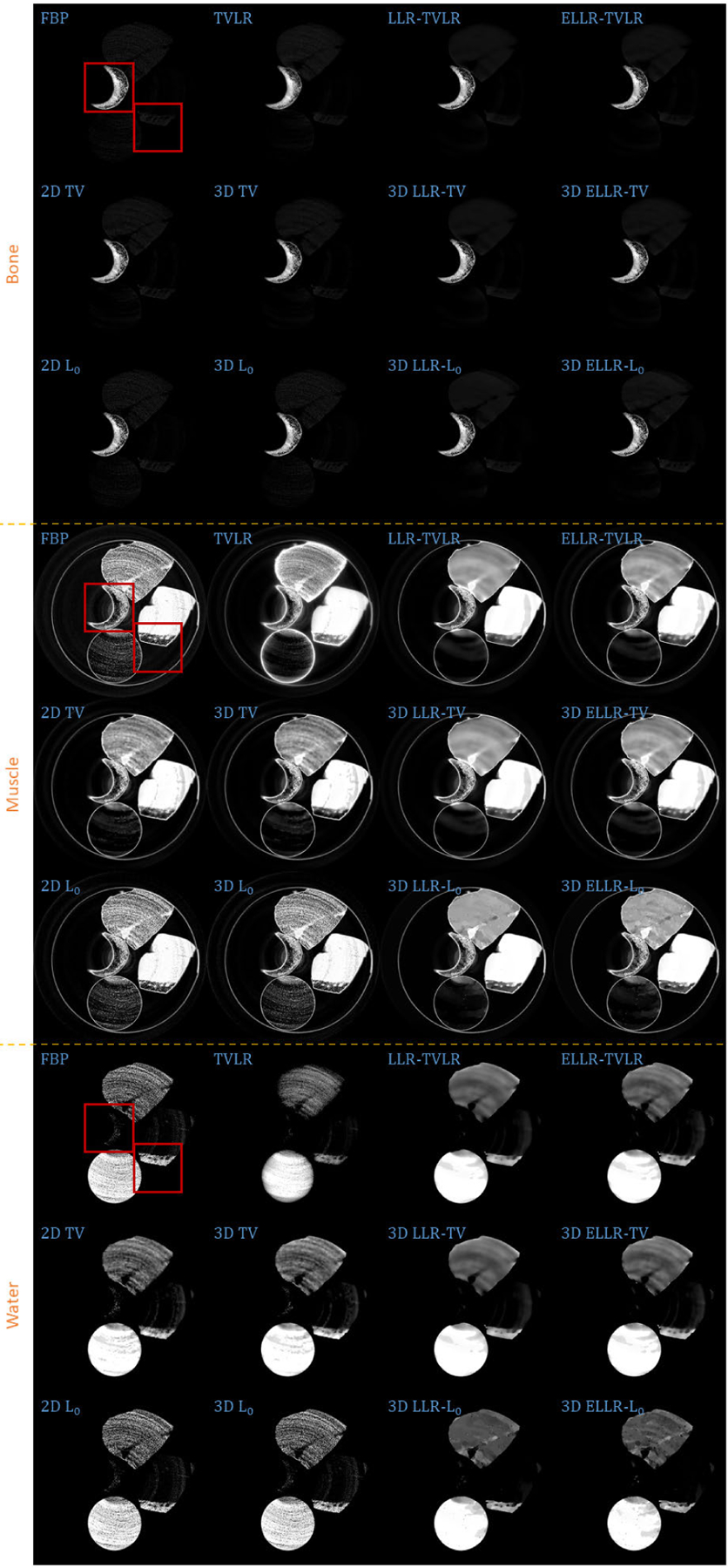
Decomposed material images of real experiment 2. The display window is [0,1] for all the results.

FIGURE 13.

Zoomed-in patches of Fig. 12, which are marked by left red boxes.

FIGURE 14.

Zoomed-in patches of Fig. 12, which are marked by right red boxes.

TABLE 2.

Quantitative comparison of decomposition accuracy for solid water in real experiment 2 (Water Group of Fig. 12).

Mean ± Std.Dev.	FBP 0.8138 ± 0.2190	TVLR 0.9702 ± 0.0567
Mean ± Std.Dev.	LLR-TVLR 0.9879 ± 0.0183	ELLR-TVLR 0.9834 ± 0.0277
Mean ± Std.Dev.	2D TV 0.9661 ± 0.0508	3D TV 0.9686 ± 0.0470
Mean ± Std.Dev.	3D LLR-TV 0.9877 ± 0.0186	3D ELLR-TV 0.9842 ± 0.0262
Mean ± Std.Dev.	2D L0 0.8246 ± 0.2048	2D L0 0.8247 ± 0.2076
Mean ± Std.Dev.	3D LLR-L0 0.9936 ± 0.0281	3D ELLR-L0 0.9905 ± 0.0354

Comparing the bone material in Figs. 8–9 and 13, the TVLR, 2D and 3D TV methods bring blurring effects to the fine bone structures. Although the FBP, 2D and 3D L₀ methods well preserve the edges, they fail to effectively remove the noise in soft tissue. Both the LLT- and ELLT-based methods work well for the dual tasks and perform consistent among all the channel images. However, the ELLT-based methods are superior in fine structure preservation (see the yellow and red arrows in Fig. 14). Comparing the numerical results in Table 2, the LLT-involved methods consistently achieve high mean value (larger than 0.98) and low standard deviation (smaller than 0.04). For 2D and 3D L₀ methods, the decomposed solid water had obvious bias with the ground truth, and even the standard variation is greater than 0.2. However, by introducing LLT, both of the evaluation metrics are dramatically improved, where the mean value is enhanced to 0.99 from 0.82 and the standard deviation drops to 0.04 from 0.20.

FIGURE 9.

Zoomed-in patches of Fig. 7, which are marked by left red boxes.

V. CONCLUSION

In this work, we mainly investigate a method to effectively establish a sparsity feature in the spectral domain, and correspondingly develop the potential applications, such as 3D gradient L₁- and L₀-norm minimization and modified TVLR method for spectral CT reconstruction. Comparing with the previous work, we refine the sparsity construction method to improve the edge preservation accuracy, propose a general optimization framework, and develop three specific minimization models. Real experiments are performed, and the results confirm the effectiveness and superiority of our proposed approaches for both image quality and decomposition accuracy.

FIGURE 10.

Zoomed-in patches of Fig. 6, which are marked by right red boxes.

Biographies

QIAN WANG (Graduate Student Member, IEEE) received the B.Sc. degree in mathematics and applied mathematics from Hebei Normal University, Hebei, China, in 2012, the M.S. degree in mathematics and information technology from Capital Normal University, Beijing, in 2016, and the Ph.D. degree in computer engineering from the Department of Electrical and Computer Engineering, University of Massachusetts at Lowell, Lowell, MA, USA, in 2020. She is currently a Postdoctoral Fellow with the Radiation Oncology Department, University of Pennsylvania. Her research interests include image reconstruction, spectral CT, medical image processing, and deep learning.

MORTEZA SALEHJAHROMI received the B.S. and M.S. degrees in electrical engineering in 2009 and 2013, respectively, and the Ph.D. degree from the University of Massachusetts at Lowell, Lowell, MA, in 2019. His research interests include image reconstruction, signal and image processing, and spectral CT.

HENGYONG YU (Senior Member, IEEE) received the bachelor’s degrees in information science and technology and computational mathematics in 1998 and the Ph.D. degree in information and communication engineering from Xi’an Jiaotong University, in 2003. He is currently a Full Professor and the Director of the Imaging and Informatics Laboratory, Department of Electrical and Computer Engineering, University of Massachusetts at Lowell. He has authored/coauthored more than 180 peer-reviewed journal articles and more than 130 conference proceedings/abstracts. According to Google Scholar Citation, his H-index is 41 and i10-index is 110. His research interests include medical imaging with an emphasis on computed tomography and medical image processing and analysis. In January 2012, he received the NSF CAREER Award for the development of CS-based interior tomography. He also serves as an Editorial Board Member for IEEE ACCESS, Signal Processing, CT Theory and Applications, and so on. He is also the Founding Editor-in-Chief of JSM Biomedical Imaging Data Papers.

REFERENCES

- [1].Wang Q, Zhu Y, and Li H, “Imaging model for the scintillator and its application to digital radiography image enhancement,” Opt. Exp, vol. 23, no. 26, pp. 33753–33776, December. 2015. [Online]. Available: http://www.opticsexpress.org/abstract.cfm?URI=oe-23-26-33753 [DOI] [PubMed] [Google Scholar]
- [2].Badea CT, Fubara B, Hedlund LW, and Johnson GA, “4-D micro-CT of the mouse heart,” Mol. Imag, vol. 4, no. 2, pp. 1–7, 2005. [DOI] [PubMed] [Google Scholar]
- [3].Badea C, Drangova M, Holdsworth DW, and Johnson G, “In vivo small-animal imaging using micro-CT and digital subtraction angiography,” Phys. Med. Biol, vol. 53, no. 19, p. R319, 2008. [DOI] [PMC free article] [PubMed] [Google Scholar]
- [4].Alvarez RE and Macovski A, “Energy-selective reconstructions in X-ray computerised tomography,” Phys. Med. Biol, vol. 21, no. 5, p. 733, 1976. [DOI] [PubMed] [Google Scholar]
- [5].Quinto ET, Ehrenpreis L, Faridani A, Gonzalez F, and Grinberg E, Radon Transforms and Tomography. Providence, RI, USA: American Mathematical Society, 2001, vol. 278. [Google Scholar]
- [6].Wang M, Zhang Y, Liu R, Guo S, and Yu H, “An adaptive reconstruction algorithm for spectral CT regularized by a reference image,” Phys. Med. Biol, vol. 61, no. 24, p. 8699, 2016. [DOI] [PMC free article] [PubMed] [Google Scholar]
- [7].Shikhaliev PM and Fritz SG, “Photon counting spectral CT versus conventional CT: Comparative evaluation for breast imaging application,” Phys. Med. Biol, vol. 56, no. 7, p. 1905, April. 2011. [DOI] [PubMed] [Google Scholar]
- [8].Persson M, Huber B, Karlsson S, Liu X, Chen H, Xu C, Yveborg M, Bornefalk H, and Danielsson M, “Energy-resolved CT imaging with a photon-counting silicon-strip detector,” Phys. Med. Biol, vol. 59, no. 22, p. 6709, 2014. [DOI] [PubMed] [Google Scholar]
- [9].Taguchi K and Iwanczyk JS, “Vision 20/20: Single photon counting X-ray detectors in medical imaging,” Med. Phys, vol. 40, no. 10, September. 2013, Art. no. 100901. [DOI] [PMC free article] [PubMed] [Google Scholar]
- [10].Schmidt TG, “Optimal ‘image-based’ weighting for energy-resolved CT,” Med. Phys, vol. 36, no. 7, pp. 3018–3027, 2009. [DOI] [PubMed] [Google Scholar]
- [11].Xu Q, Yu H, Bennett J, He P, Zainon R, Doesburg R, Opie A, Walsh M, Shen H, Butler A, Butler P, Mou X, and Wang G, “Image reconstruction for hybrid true-color micro-CT,” IEEE Trans. Biomed. Eng, vol. 59, no. 6, pp. 1711–1719, June. 2012. [DOI] [PMC free article] [PubMed] [Google Scholar]
- [12].Xu Q, Yu H, Mou X, Zhang L, Hsieh J, and Wang G, “Low-dose X-ray CT reconstruction via dictionary learning,” IEEE Trans. Med. Imag, vol. 31, no. 9, pp. 1682–1697, September. 2012. [DOI] [PMC free article] [PubMed] [Google Scholar]
- [13].Zhao B, Gao H, Ding H, and Molloi S, “Tight-frame based iterative image reconstruction for spectral breast CT,” Med. Phys, vol. 40, no. 3, February. 2013, Art. no. 031905. [DOI] [PMC free article] [PubMed] [Google Scholar]
- [14].Chu J, Li L, Chen Z, Wang G, and Gao H, “Multi-energy CT reconstruction based on low rank and sparsity with the split-Bregman method (MLRSS),” in Proc. IEEE Nucl. Sci. Symp. Med. Imag. Conf. Rec. (NSS/MIC), October. 2012, pp. 2411–2414.
- [15].Zhang Y, Mou X, Wang G, and Yu H, “Tensor-based dictionary learning for spectral CT reconstruction,” IEEE Trans. Med. Imag, vol. 36, no. 1, pp. 142–154, January. 2017. [DOI] [PMC free article] [PubMed] [Google Scholar]
- [16].Wu W, Zhang Y, Wang Q, Liu F, Chen P, and Yu H, “Low-dose spectral CT reconstruction using image gradient ℓ0–norm and tensor dictionary,” Appl. Math. Model, vol. 63, pp. 538–557, November. 2018. [DOI] [PMC free article] [PubMed] [Google Scholar]
- [17].Salehjahromi M, Zhang Y, and Yu H, “Iterative spectral CT reconstruction based on low rank and average-image-incorporated BM3D,” Phys. Med. Biol, vol. 63, no. 15, August. 2018, Art. no. 155021. [DOI] [PMC free article] [PubMed] [Google Scholar]
- [18].Wu W, Liu F, Zhang Y, Wang Q, and Yu H, “Non-local low-rank cube-based tensor factorization for spectral CT reconstruction,” IEEE Trans. Med. Imag, vol. 38, no. 4, pp. 1079–1093, April. 2019. [DOI] [PMC free article] [PubMed] [Google Scholar]
- [19].Niu S, Bian Z, Zeng D, Yu G, Ma J, and Wang J, “Total image constrained diffusion tensor for spectral computed tomography reconstruction,” Appl. Math. Model, vol. 68, pp. 487–508, April. 2019. [Google Scholar]
- [20].Yao L, Zeng D, Chen G, Liao Y, Li S, Zhang Y, Wang Y, Tao X, Niu S, Lv Q, Bian Z, Ma J, and Huang J, “Multi-energy computed tomography reconstruction using a nonlocal spectral similarity model,” Phys. Med. Biol, vol. 64, no. 3, January. 2019, Art. no. 035018. [DOI] [PubMed] [Google Scholar]
- [21].Wang Q, Wu W, Deng S, Zhu Y, and Yu H, “Locally linear transform based three-dimensional gradient-norm minimization for spectral CT reconstruction,” Med. Phys, vol. 47, no. 10, pp. 4810–4826, October. 2020. [Online]. Available: https://aapm.onlinelibrary.wiley.com/doi/abs/10.1002/mp.14420 [DOI] [PubMed] [Google Scholar]
- [22].He K, Sun J, and Tang X, “Guided image filtering,” IEEE Trans. Pattern Anal. Mach. Intell, vol. 35, no. 6, pp. 1397–1409, June. 2013. [DOI] [PubMed] [Google Scholar]
- [23].Bauschke HH and Borwein JM, “On projection algorithms for solving convex feasibility problems,” SIAM Rev, vol. 38, no. 3, pp. 367–426, September. 1996. [Google Scholar]
- [24].Xu L, Lu C, Xu Y, and Jia J, “Image smoothing via L0 gradient minimization,” ACM Trans. Graph, vol. 30, no. 6, pp. 174:1–174:12, 2011. [Google Scholar]
- [25].Mendonça PR, Bhotika R, Maddah M, Thomsen B, Dutta S, Licato PE, and Joshi MC, “Multi-material decomposition of spectral CT images,” Proc. SPIE, vol. 7622, March. 2010, Art. no. 76221W. [Google Scholar]
- [26].Granton PV, Pollmann SI, Ford NL, Drangova M, and Holdsworth DW, “Implementation of dual- and triple-energy cone-beam micro-CT for postreconstruction material decomposition,” Med. Phys, vol. 35, no. 11, pp. 5030–5042, October. 2008. [DOI] [PubMed] [Google Scholar]