The Use of Local and Nonlocal Priors in Bayesian Test-based Monitoring for Single-arm Phase II Clinical Trials

Abstract

Bayesian sequential monitoring is widely used in adaptive phase II studies where the objective is to examine whether an experimental drug is efficacious. Common approaches for Bayesian sequential monitoring are based on posterior or predictive probabilities and Bayesian hypothesis testing procedures using Bayes factors. In the first part of the paper, we briefly show the connections between test-based (TB) and posterior probability-based (PB) sequential monitoring approaches. Next, we extensively investigate the choice of local and nonlocal priors for the TB monitoring procedure. We describe the pros and cons of different priors in terms of operating characteristics. We also develop a user-friendly Shiny application to implement the TB design.

1. Introduction

Phase II clinical trials play a critical role in drug development. The objective of phase II clinical trials is to evaluate the therapeutic effect of a new treatment and screen out inefficacious agents. Phase II trials commonly use a short-term, dichotomous endpoint to characterize the patient clinical response to treatment. For example, a binary objective response endpoint can be used to indicate whether patients have achieved a complete or partial response within a predefined treatment course. If the new treatment shows a promising treatment effect (i.e., has a desirable response probability), additional large-scale confirmatory trials can be conducted.

In general, phase II studies can be performed using either frequentist or Bayesian designs.^1,2 The frequentist approaches treat the response probability of the new treatment as a fixed, yet unknown parameter.^3–5 The most well-known frequentist phase II design is Simon’s two-stage design.⁶ In this design, n₁ patients are enrolled in stage I. If there are r₁ or fewer responses, terminate the trial early and conclude that the drug is not promising; otherwise, enroll an additional n₂ patients in stage II and, if more than r responses are observed, claim that the drug is promising. The parameters of Simon’s design are optimized to minimize the expected sample size (the optimal design) or the maximum sample size (the minimax design) under the null hypothesis that the treatment is not efficacious, given specified type I and type II error rates. Simon’s two-stage design is widely adopted in phase II trials. Numerous generalizations or extensions of Simon’s two stage design have been proposed. Examples include the three-stage design,⁷ the design based on a composite null hypothesis,⁸ the optimal adaptive design,⁹ and the multiple-arm design¹⁰ among others.

Most of the frequentist phase II designs only have two or three stages, with the design parameters determined based on numerical searching. These designs are rigid in the sense that they do not allow any deviation from the original design. For example, for the Simon’s design, the “go/no-go” decisions can only be made at the predetermined interim time, and the design will not stop the trial early, even when observed data have clearly indicated that the drug is futile. To safe guard patients from futile treatments and accelerate the development of efficacious drugs, it is critical to make adaptive decisions based on the accumulated data throughout the trial in a timely fashion.

When more interim analyses are desired, Bayesian methods become particularly appealing due to their “we learn as we go” nature.¹¹ In Bayesian phase II designs, the treatment effect is considered as an unknown random variable, and the Bayesian inference can be adaptively and timely made, as long as new data are observed. As a result, Bayesian designs usually are more flexible in facilitating multiple interim decisions. In addition, frequentist methods require a penalty for each look of the data, but there are no such hurdles for interim analyses in a Bayesian perspective.¹²

Due to the appealing feature of flexibility, there have been vast developments in Bayesian phase II clinical trial designs in recent years.^13–22 Overall, Bayesian sequential monitoring approaches can be divided into two categories: posterior (or predictive) probability-based (PB) or Bayesian hypothesis test-based (TB). PB designs refer to those, for which the go/no-go decisions are made based on the Bayesian posterior (or predictive) probability that the treatment is futile or effective. If such a probability is greater than a pre-specified probability cutoff, then the trial can be terminated early, as the experimental treatment is likely to be futile or promising. If this probability is small, however, then there is inadequate information to deliver a conclusion, and the trial continues to collect more data (more details on PB designs are provided in Section 2.1). On the other hand, TB designs refer to those that make the go/no-go decisions based on the Bayesian hypothesis testing framework with Bayes factor (specific examples are provided in Section 2.2). Although Johnson and Cook¹⁴ argued that the use of Bayes factor in sequential monitoring can gain more efficiency compared to the PB approach, while also eliminating a potential source of bias often caused by prior-data conflict, the research on the TB approach for phase II trials is lacking. Limited examples include the two-stage Bayes factor based design²³ and the design to identify the maximum effective dose.²⁴ To get more insight into TB monitoring, in the first part of the paper we briefly show the connection between the TB and PB approaches and their main difference.

An issue that was largely overlooked regarding the Bayesian approaches is the choice of prior distributions for TB designs. For TB designs, prior distributions are required to quantify the initial uncertainty of the unknown parameter under the hypotheses. For example, H₀ : p ~ π₀(p) versus H₀ : p ~ π₁(p) with support on Θ₀ and Θ₁, respectively. The prior distributions under the alternative can be classified into local priors and nonlocal priors.²⁵ A local prior refers to a probability density that is positive at the parameter space that is consistent with the null hypothesis, i.e., π₁(p ∈ Θ₀) > 0. With a binary endpoint, the commonly used Beta distribution falls into the category of local priors, as the Beta prior has a positive probability in the [0,1] support. Similarly, meta-analytical prior (MAP)²⁶ and robust MAP (rMAP)²⁷ are local priors. A problem associated with using a local prior in Bayesian hypothesis testing is that it accumulates evidence in favor of the true null hypothesis at a much slower rate, as compared to favoring a true alternative hypothesis.²⁵ This indicates that when futility monitoring is of interest in a trial, using local priors has a smaller likelihood to early terminate a futile treatment. To address this issue, a class of nonlocal priors were proposed, among which the flexible inverse moment (iMOM) density is a classic example.^14,25 With the use of the nonlocal prior, it expects to require smaller number of patients to terminate a trial for futility when the drug is indeed futile, as the nonlocal prior accumulates the evidence in favoring of the true null at a much faster rate than local priors.

In the second part of this paper, we examine the effects of local and nonlocal priors on the TB monitoring procedure and demonstrate the pros and cons of each prior through extensive simulations. We found that the iMOM prior and rMAP with a weakly informative mixture component²⁷ yield desirable operating characteristics in the TB design setting. Specifically, iMOM is ideal in the sequential monitoring, as it has a greater chance to stop a trial at earlier interim analyses when the drug is futile, while rMAP is the most robust to prior-data conflict when parameter estimation is of interest after a trial completes.

The rest of the paper is organized as follows. In Section 2, we first provide an overview of different Bayesian monitoring approaches and then show the relationship between PB monitoring and TB monitoring. In Section 3, we describe prior specification for Beta distribution, MAP, rMAP, and iMOM density, and methods to determine effective sample size (ESS). In Section 4, we conduct extensive simulations to examine the operating characteristics of the TB monitoring using different priors. Sensitivity analyses are considered in Section 5. In Section 6, we provide a user-friendly software to design to facilitate the use of TB sequential monitoring. In Section 7, we extend the TB method to simultaneously monitor efficacy and toxicity. We conclude the study in Section 8.

2. Sequential monitoring

2.1. Bayesian posterior (or predictive) probability based (PB) monitoring

In a phase II trial, let n denote the number of patients and Y denote the number of responses observed. The treatment effect is quantified by estimating the probability of clinical response (p = Y/n). The number of response Y is usually modeled as a binomial random variable, i.e., Y ~ Binom(n, p). Given the observed value D_n = (y, n), the binomial likelihood function is $f\left(D_n\mid p\right)=\left(\begin{array}{l}n\hfill \\ y\hfill \end{array}\right)p^y{(1-p)}^{n-y}$, where y is the observed number of responses. In Bayesian inference, all the information about the parameter is contained in the posterior distribution of p, which can be calculated using the Bayes’ theorem as follows:

$$\pi \left(p\mid D_n\right)=\frac{f\left(D_n\mid p\right)\pi (p)}{\int f\left(D_n\mid p\right)\pi (p)dp},0\le p\le 1.$$ (2.1)

Here, π(p) is the prior distribution for the unknown parameter p, which characterizes all available information before conducting the trial. For phase II oncology studies, we do not always have prior information on p, so non-informative priors are always used. Nevertheless, we also consider the situation of if informative priors are available, and assess the sensitivity of different approaches to informative priors.

Let p₀ denote a clinically uninteresting response probability or the response probability of the standard of care, and let p₁ represent a desirable target response probability. In general, the go/no-go decisions for the PB approach can be made based on either the posterior probability or the predictive probability that the experimental drug has a higher response probability than p₀ based on the observed data accumulated by the interim decision-making time. For example, if superiority monitoring is of interest, the posterior probability that the response probability of the experimental drug (p) exceeds the response probability of the standard treatment (p₀) by a prespecified improvement δ, i.e., Pr(p > (p₀ + δ) | D), can be calculated continuously at each interim decision-making time when the data have accumulated. Then the trial can be stopped early for superiority if Pr(p > (p₀+δ) | D_n) > r_e, where r_e is a probability cutoff. Similarly, if futility stopping is desired, the trial can be stopped early for futility if Pr(p < (p₀ + δ) | D_n) > r_f, where r_f is also a probability cutoff. In many cases, the probability cutoffs r_f and r_e take fixed values at 0.90 or 0.95. Alternatively, they can be calibrated through simulation to satisfy certain prespecified type I/II error constraints. The value of δ should be chosen to reflect the clinical need. In this paper, we only consider p₀ as a prespecified point, and fix δ = 0. If the stopping criteria is not satisfied, then there is not adequate information to deliver any conclusion, so the trial continues to collect more data until reaching the pre-specified sample size. Generalization of this Bayesian monitoring procedure can be found in Heitjan,¹³ Thall et al.,¹⁹ and Zhou et al.,²² among others.

In addition to the posterior probability, Bayesian predictive probability serves as a good alternative tool to conduct interim decision monitoring. The decision rules of the predictive probability monitoring procedure mimic that of the posterior probability monitoring procedure.¹⁵ Like posterior probability monitoring, predictive probability monitoring is more adaptable than traditional multi-stage designs, and it has been extended to different trial settings.^21,28,29

2.2. Bayesian hypothesis test-based (TB) monitoring

Another alternative Bayesian monitoring approach is developed on the basis of the Bayesian hypothesis testing procedure.¹⁴ Specifically, consider the following hypotheses:

$$H_0:p\le p_0\text{\hspace{1em} versus \hspace{1em}}{H}_1:p>p_0,$$ (2.2)

where under the null hypothesis H₀, the treatment effect is deemed unpromising. The value of p₀ is assumed to be known and fixed in this study. Under the Bayesian framework, the Bayes factor serves as a natural quantity to measure the strength of evidence for a hypothesis relative to another one.³⁰ Specifically, the Bayes factor in favor of H₁ (denoted as BF₁₀) can be calculated as

$$B{F}_{10}=\frac{\text{Pr}\left(D_n\mid H_1\right)}{\text{Pr}\left(D_n\mid H_0\right)}=\frac{{\int }_{p_0}^{1}f\left(D_n\mid p\right)\pi \left(p\mid H_1\right)\text{d}p}{{\int }_0^{p_0}f\left(D_n\mid p\right)\pi \left(p\mid H_0\right)\text{d}p},$$ (2.3)

where f(D_n | p) is the data likelihood and π(p | H_j) is the prior distribution of p under H_j, j = 0, 1. That is, the Bayes factor is the ratio of likelihood averaged over the prior under H₁ and H₀.

Under the Bayesian hypothesis testing framework, a decision to reject the null hypothesis occurs only when the Bayes factor in favor of the alternative hypothesis exceeds a pre-specified evidence level. A greater BF₁₀ indicates a stronger evidence for H₁. Alternatively, we can define the Bayes factor as BF₀₁ = Pr(D_n | H₀)/Pr(D_n | H₁). In this case, a larger BF₀₁ indicates a greater evidence for H₀. Table S.1 shows the general interpretation of the Bayes factor as the strength of evidence for hypothesis testing.³¹ Johnson and Cook¹⁴ showed that when the prior ascribed to the hypothesis is not consistent with the data, the Bayes factor in favor of the alternative hypothesis will almost always be smaller than it could have been with a correctly-specified prior under H₁. As a result, compared to PB monitoring that is based on posterior probability intervals, TB monitoring based on Bayes factors can automatically adjust the bias induced by overly optimistic priors. This property is of practical use, especially from a regulatory perspective.

At each interim decision-making time, the TB monitoring procedure adaptively tests the hypotheses (2.2) and makes go/no-go decisions as follows:

• Stop the trial to claim superiority of the new treatment if BF₁₀ > γ_e.

• Stop the trial to claim futility of the new treatment if BF₀₁ > γ_f,

The γ_e and γ_f are pre-specified values that represent substantial evidence in favor of H₁ and H₀, respectively, or are calibrated through simulation to satisfy certain type I/II error constraints.

2.3. Relationship between PB monitoring and TB monitoring

As previously mentioned, PB monitoring is based on the posterior probability that the response probability is greater (or less) than the reference response probability given observed data, while TB monitoring is based on the evidence contained in the data in favor of one hypothesis relative to another one. Nevertheless, the two monitoring approaches are closely related. The first link can be seen through the way the Bayes factor is calculated. Besides the formula (2.3), another way to calculate BF₁₀ is using Bayes’s theorem, by which we have

$$\text{Pr}\left(H_1\mid D_n\right)=\frac{\text{Pr}\left(D_n\mid H_1\right)\text{Pr}\left(H_1\right)}{\text{Pr}\left(D_n\mid H_1\right)\text{Pr}\left(H_1\right)+\text{Pr}\left(D_n\mid H_0\right)\text{Pr}\left(H_0\right)},$$

such that

$$\underset{\text{Posterior odds }}{\underbrace{\frac{\text{Pr}\left(H_1\mid D_n\right)}{\text{Pr}\left(H_0\mid D_n\right)}}}=\underset{\text{Bayes factor }}{\underbrace{\frac{\text{Pr}\left(D_n\mid H_1\right)}{\text{Pr}\left(D_n\mid H_0\right)}}}\times \underset{\text{Prior odds }}{\underbrace{\frac{\text{Pr}\left(H_1\right)}{\text{Pr}\left(H_0\right)}}}.$$ (2.4)

It follows from (2.4) that the Bayes factor is simply the posterior odds of H₁ to its prior odds. When no or little prior information can be borrowed, it is natural to assume a priori that the hypotheses are equally likely, i.e., the prior hypothesis probabilities Pr(H₀) = Pr(H₁) = 1/2. In this case, the Bayes factor BF₁₀ is equivalent to the posterior odds in favor of H₁. The relationship between the Bayes factor and the posterior odds provides the first connection between the TB and PB approaches.

Another connection between the two approaches can be revealed directly by the monitoring rules. Let π(p) = Pr(H₀)π(p | H₀)+Pr(H₁)π(p | H₁) be the overall prior distribution, and let π(p | D_n) be the overall posterior distribution of p at the interim sample size of n, which is calculated based on the observed data D_n and the overall prior π(p). Then the posterior probability of H_j can be computed as $\text{Pr}\left(H_j\mid D_n\right)={\int }_{H_j}\pi \left(p\mid D_n\right)\text{d}p,j=0,1$. According to the Bayes factor definition, for futility monitoring, we have

$$\begin{gathered} \frac{\text{Pr}\left(D_n\mid H_0\right)}{\text{Pr}\left(D_n\mid H_1\right)}>{\gamma }_f \\ \iff \frac{\text{Pr}\left(H_0\mid D_n\right)}{\text{Pr}\left(H_1\mid D_n\right)}\frac{\text{Pr}\left(H_1\right)}{\text{Pr}\left(H_0\right)}>{\gamma }_f \\ \iff \text{Pr}\left(H_0\mid D_n\right)>\frac{{\gamma }_f\text{Pr}\left(H_0\right)\text{Pr}\left(H_1\mid D_n\right)}{\text{Pr}\left(H_1\right)} \\ \iff \text{Pr}\left(p\le p_0\mid D_n\right)>\frac{{\gamma }_f\text{Pr}\left(H_0\right)\text{Pr}\left(p>p_0\mid D_n\right)}{\text{Pr}\left(H_1\right)} \\ \iff \text{Pr}\left(p\le p_0\mid D_n\right)>\frac{{\gamma }_f}{{\gamma }_f+\text{Pr}\left(H_1\right)/\text{Pr}\left(H_0\right)}\equiv {\gamma }_f^{\prime }. \end{gathered}$$

Here, ${\gamma }_f^{\prime }$ depends on the prior odds Pr(H₁)/Pr(H₀), indicating the close link between the TB and PB approaches. A similar proof can be done for superiority monitoring. The main difference between the two approaches lies in the prior distribution. Specifically, PB usually assigns a continuous distribution (or a mixture of continuous distributions) in the probability support of [0, 1], while TB usually has a mixture overall prior for p (e.g., π(p) = Pr(H₀)π(p | H₀) + Pr(H₁)π(p | H₁)).

It must be noted that no matter which approach is adopted for a phase II design, sample size determination is crucial in order to maintain certain operating characteristics, similar to what is in frequentist approaches, such as type I and II error rates. This can be done through simulation in the Bayesian setting. In addition, the sample size at which the first interim is conducted (referred to as “burn-in” size) is critical. In general, it should be no less than the actual cohort size for subsequent analysis. An appropriate choice of cohort size should be carefully chosen to maintain desirable operating characteristics. We dedicate more details to this topic in Section 5 to show the impact of sample size, burn-in size, and cohort size.

3. Prior specification

Prior specification is critical to the performance of Bayesian inference. Recently, the US Food and Drug Administration³² announced a draft guideline for industry and highlighted the importance of the evaluation of prior distribution on innovative trial designs. In early-phase trials when the sample size is typically small, the use of prior information for Bayesian designs could be a double-edged sword. Different prior distributions may lead to varied interim decisions or final conclusions.³³ If the prior is consistent with the observed data, it would increase the trial efficiency and render more accurate decision making. In contrast, if the prior is not congruent with the current data (referred to as “prior-data conflict”), inference may be subject to bias and decisions could be wrong. Hence, the choice of prior distribution should be carefully made according to the clinical setting, expert knowledge, and sufficient simulation studies.

The choice of prior has been well explored under the PB design for both one-arm and randomized two-arm settings with the purpose of improving the efficiency of a design, while also alleviating prior-data conflict. Classical examples include the power prior,³⁴ modified power prior,³⁵ commensurate prior,^36,37 meta-analytic-predictive (MAP) prior,²⁶ robust MAP,²⁷ and empirical MAP,³⁸ among others. A discussion of the connections among some of the priors can be found in Neuenschwander et al.³⁹ However, this is a largely overlooked issue in the choice of prior distributions under the TB design setting. In this section, we describe several prior distributions that will be thoroughly examined in the TB monitoring procedure.

3.1. Beta distribution

Since the primary endpoint in phase II trials is usually binary, a natural choice of the prior for the response probability (p) is the Beta prior due to the conjugacy. The use of a conjugate prior simplifies the computation for posterior distribution, as it gives a closed-form expression for the posterior. Suppose that the prior distribution is p ~ Beta(a, b), where a and b are the hyperparameters. The quantity a/(a + b) reflects the prior mean, while the size of a + b indicates how informative the prior is. The larger the value of a + b, the more informative the prior. In many cases, a Beta(1, 1) is used as a non-informative prior, which is equivalent to the Uniform[0,1] distribution. Given the observed data D_n = (y, n), the posterior distribution of p is still a Beta distribution, i.e., p | D_n ~ Beta(y + a, n − y + b). Such a beta-binomial model has been widely applied in early-phase trial designs.^8,15,40–42

3.2. Meta-analytical-predictive prior

The basic idea of a meta-analytical-predictive (MAP) prior is to obtain a prior distribution for the parameter of interest using a Bayesian hierarchical model, based on available historical trials.²⁶ The density of the MAP prior is typically not in a closed-form expression. To simplify the density estimation, Schmidli et al.²⁷ proposed to use a mixture conjugate prior to approximate the MAP prior. Specifically, suppose there are K historical trials available to derive the prior, and the information borrowed from each historical trial can be represented using a Beta distribution with shape parameters a_k and b_k, k = 1, ⋯ ,K. Then the MAP prior can be determined as

$$\pi (p)=\sum _{k=1}^K{w}_k\mathit{\text{Beta}}\left(p\mid a_k,b_k\right),$$ (3.1)

where w_k, k = 1, ⋯ ,K is a pre-determined weight with ${\sum }_{k=1}^K{w}_k=1$; a_k and b_k are the shape parameters of the Beta distribution determined by the k^th historical trial. When K = 1, the MAP prior resorts to the standard Beta prior. To acknowledge the possibility of prior-data conflict, Schmidli et al.²⁷ proposed the robust MAP prior by adding a vague Beta prior with shape parameters a₀ and b₀ to (3.1) as follows:

$$f(p)=w_r\sum _{k=1}^K{w}_k\mathit{\text{Beta}}\left(p\mid a_k,b_k\right)+\left(1-w_r\right)\mathit{\text{Beta}}\left(p\mid a_0,b_0\right),$$ (3.2)

where the weight for the MAP prior (i.e., w_r) can be specified using a larger value (e.g., w_r = 0.9) if there is a strong belief in the MAP prior. If there is more uncertainty regarding MAP, then a smaller value of w_r is desired (e.g., w_r = 0.5).

3.3. The inverse moment (iMOM) density

The Beta distributions, MAP, rMAP priors have a non-negligible amount of density to the parameter space that is consistent with the null hypothesis in the TB setting, and thus they belong to the category of local prior. Johnson and Rossell²⁵ proposed the inverse moment (iMOM) prior density, which is a nonlocal prior. When the parameter of interest is response probability (p), a common choice of the iMOM density takes the following form:

$$\pi \left(p;p_0,k,\nu ,\tau \right)=\frac{k{\tau }^{\nu /2}}{\Gamma (\nu /2k)}{\left[{\left(p-p_0\right)}^2\right]}^{-(\nu +1)/2}\text{exp}\left\{-{\left[\frac{{\left(p-p_0\right)}^2}{\tau }\right]}^{-k}\right\}\frac{1}{C}$$ (3.3)

where p₀ is the null value, p ∈ [0, 1], k > 0, ν > 0, τ > 0 are the parameters that jointly define the iMOM density, and C is the normalized constant.

The function form of the iMOM density is related to inverse gamma density function. Thus its behavior near p₀ is similar to the behavior of an inverse gamma density near 0. Figure 1 shows an example of the iMOM prior ascribed to H₁ : p > p₀ with p₀ = 0.2. As shown, when p = p₀, we have π(p; p₀, k, ν, τ) = 0. Moreover, the iMOM density approaches zero exponentially as p gets closer to p₀. More examples are provided in Figure S.1, which shows that the k and τ behave like the scale parameter in inverse gamma function. That is, as one of the two parameters increases, the iMOM density has values close to zero in a larger parameter space nearby H₀. Meanwhile, the parameter ν is similar to the shape parameter in the inverse gamma function: a larger value of ν comes with a lighter tail and higher peak of the mode.

Figure 1:

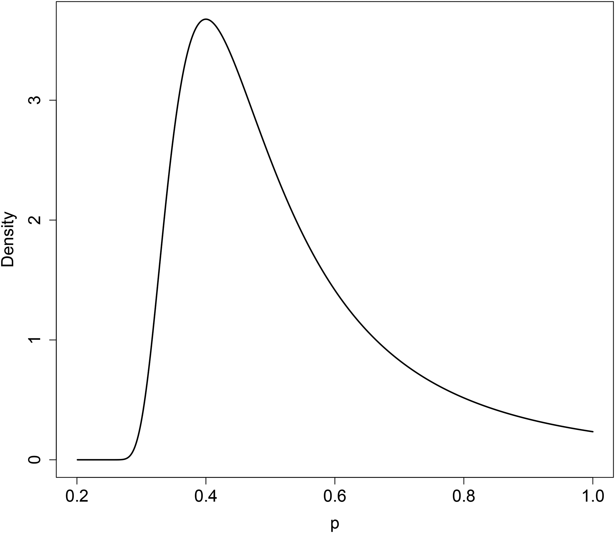
Example of the iMOM prior restricted in the range of (0.2, 1] with k = 1, ν = 2, and τ = 0.06.

3.4. Prior effective sample size

A fundamental aspect of using the Bayesian approach is to quantify the amount of information contained in the prior.⁴³ This is measured by the effective sample size (ESS), which is defined as the number of hypothetical patients associated with the prior distribution. For the standard Beta prior (MAP prior with one historical study) or rMAP prior, the ESS is easily determined as a function of the shape parameters.⁴⁴ But it is not straightforward to estimate the ESS for the iMOM prior. Various variance-ratio based approaches have been proposed to approximate the ESS.^26,45–47 Morita et al.⁴⁸ proposed an information-based ESS, in which both Fisher information and the information of the prior are utilized to calculate the ESS. Neuenschwander et al.⁴⁴ proposed the expected-local-information-ratio (ELIR) method, which is predictively consistent such that the expected posterior-predictive ESS for a sample of size N should equal the sum of the prior ESS and N. While the ELIR method is ideal and can be easily obtained for many distributions, it is not applicable to the iMOM prior, because the ELIR for iMOM does not exist. We used Morita’s method to estimate ESS in this paper.⁴⁸

Let i(π(p)) denote the information of the prior distribution π(p), and i(π₀(p)) be the information of a large-variance prior π₀(p) that has the same mean $\overline{p}$ as π(p), where we used ${\pi }_0(p)=\mathit{\text{Beta}}\left(a_0^{*},b_0^{*}\right)$ with $a_0^{*}$ and $b_0^{*}$ chosen such that $a_0^{*}+b_0^{*}={10}^{-4}$ and $a_0^{*}/\left(a_0^{*}+b_0^{*}\right)=\overline{p}$. Let i_F(Y_m; p) be the observed Fisher information for m information units in the prior.

$$i_F\left(Y_m;p\right)=-\frac{d^{2}log\left(f\left(Y_m\mid p\right)\right)}{d{p}^2},$$

where f(Y_m | p) is the probability mass function of the random variable Y_m, which is assumed to follow a binomial distribution Binom(m, p). ESS is then approximated by the integer that minimizes $\left|i\left({\pi }_0(\overline{p})\right)+E_{Y_m}\left[i_F\left(Y_m;\overline{p}\right)\right]-i(\pi (\overline{p}))\right|$.

4. Simulation

4.1. Simulation setting

We assessed the performance of the TB design under various prior specifications through extensive simulations. Considering a hypothetical phase II trial, we assumed that the response probability for the standard of care was 0.2 and the new treatment was anticipated to have a larger response probability of 0.4. Following Johnson and Cook,¹⁴ we assigned a point mass density with p = 0.2 under the null hypothesis H₀ and tested various prior densities under the alternative H₁. The prior densities under H₁ include the iMOM prior, MAP with K = 1, rMAP with w_r = 0.9 (rMAP_mix90), rMAP with w_r = 0.5 (rMAP_mix50), and the commonly used Uniform prior. We included the Uniform prior to demonstrate how the trial operating characteristics would be improved by incorporating informative priors. All the informative priors ascribed to H₁ had a mode of 0.4. The amount of information contained in the prior was reflected by the prior ESS calculated using Morita’s method.⁴⁸ We considered both a weakly informative prior with ESS=5 and a strongly informative prior with ESS=20. The priors were specified as in Table 1.

Table 1:

Prior specifications for simulation study

Design	ESS=5	ESS=20
iMOM	π(p; k = 1.24, ν = 2.48, τ = 0.0526)	π(p; k = 2.04, ν = 4.08, τ = 0.0445)
MAP	Beta(2.2, 2.8)	Beta(8.2, 11.8)
rMAP_mix90	0.9 × Beta(2.2, 2.8) + 0.1 × Beta(1,1)	0.9 × Beta(8.2,11.8) + 0.1 × Beta(1,1)
rMAP_mix50	0.5 × Beta(1.8, 2.2) + 0.5Beta(1,1)	0.5 × Beta(7.8,11.2) + 0.5 × Beta(1,1)

In addition to comparing various priors under the TB design setting, we also included a classic PB design developed by Thall and Simon,¹⁸ which we referred to as the TS design. The TS design used the MAP priors described above for sequential monitoring. We considered 13 scenarios with the true response probability ranging from 0 to 0.6, with an interval space of 0.05. The operating characteristics were assessed based on 10, 000 simulated trials for each scenario. Under each scenario, we assumed that the trial enrolled at most N patients (N = 50) and patients entered the trial with a cohort size of ten. The first interim analysis was carried out when 20 patients were treated and had their outcomes evaluated, then an interim analysis was conducted after every ten additional patients. For the TB design, the trial was early terminated for superiority if BF₁₀ ≥ γ_e; early terminated for futility if BF₀₁ ≥ γ_f; and otherwise continued until the maximum sample size (N) was reached. In contrast, the TS design stopped the trial for superiority if Pr(p > p₀ | D_n) > r_e and for futility if Pr(p < p₀ | D_n) > r_f. The cutoffs (γ_e = 3, γ_f = 9, r_e = 0.988, r_f = 0.3) were chosen given ESS=5, such that the TB design with the iMOM prior and the TS design have the same probability of claiming superiority when H₀ is true (p = 0.2) and claiming futility when the drug is actually efficacious (i.e., p = 0.4). The same cutoffs were used when ESS=20 to demonstrate the performance of different informative priors given fixed strength of evidence (i.e., same cutoffs).

We evaluated three different metrics for the comparison for all the designs considered: (1) the probability of claiming superiority, which was defined as the percentage of simulated trials claiming that the treatment is efficacious; (2) the probability of claiming futility, which was defined as the percentage of simulated trials claiming that the treatment is futile; and (3) the average number of patients treated in the 10, 000 simulated trials for each scenario. In addition to the overall probability of claiming superiority or futility, we also summarized the probabilities at each interim look, as well as at the final analysis. If larger probabilities of making a correct decision are observed at earlier interim analyses, it indicates a more efficient design. Here, the correct decision refers to claiming superiority under H₁ and claiming futility under H₀.

After the trial is stopped for either futility or superiority, inference on the response probability is of interest. Thus it is also important to assess the robustness of the priors in terms of parameter estimation. We examined the bias, root mean square error (RMSE), and 95% credible interval coverage for using the different prior distributions.

4.2. Simulation results

Figure 2 shows the operating characteristics of the TB design with different prior distributions assumed under H₁, as well as that of TS. For TB with ESS=5, we note comparable probabilities in claiming superiority among the TS design and the TB designs with iMOM, MAP, rMAP mix90, and rMAP mix50 priors. The TB design with a non-informative prior has a smaller probability of claiming superiority. In terms of claiming futility when the drug is futile, the most desirable prior under the TB design appears to be iMOM, followed by rMAP mix50, rMAP mix90, and MAP, regardless of ESS values. When the strength of evidence is fixed (ESS=20), compared to the TB design, the TS design has a larger probability to claim superiority when the drug is efficacious, but also it is subject to a higher false positive rate (panel b1). Moreover, the TS design is less likely to stop for futility (panel b2).

Figure 2:

Operating characteristics of sequential monitoring using the Bayes factor and TS design under a weakly informative prior (ESS=5) and strongly informative prior (ESS=20).

Notably, the uniform prior under the simulation setting behaves abysmally, i.e., the trial never terminates for futility, regardless of the true response probability. This indicates that, given the same strength of evidence (i.e., same Bayes factor cutoffs) under the TB design, using uniform prior is less likely to claim for futility than other priors. Section S.3 shows that if we were to control the type I error rate for each prior separately, then we would not see a difference in probability of claiming superiority or futility. This is because type I error control eliminates the borrowing of favorable prior information (comparing non-informative versus informative) and disguises the dissimilarity between different priors. This finding is consistent with that in Quan et al.,⁴⁹ and it suggests that when the use of an informative prior is desired, the requirement of strict type I error control has to be replaced by more appropriate metrics.⁵⁰ In this study, we control the strength of evidence (using the same cutoffs for different priors) in the simulation to reveal the difference of the operating characteristics for various priors.

In terms of average sample size, the TB design using iMOM prior enrolls fewer patients on average (panels a3 and b3 of Figure 2). The TS design requires a smaller sample size if the treatment is indeed efficacious (e.g., p = 0.4) when ESS=20, but it will need a larger sample size when the drug is futile (e.g., p = 0.2) due to the small likelihood of stopping for futility, as demonstrated in panels a2 and b2 of Figure 2.

Figure 3 shows that TB with different informative priors has a similar probability of stopping for superiority at each interim analysis, while using the uniform prior has the smallest chance of stopping for superiority at the first interim analysis. When ESS=5, the TS design has similar behavior to the TB design in the probability of claiming superiority at each interim analysis. When ESS=20, compared to the TB design with informative priors, the TS design has the greatest probability of claiming superiority, but the smallest probability of claiming futility. Because the prior is in favor of H₁, it requires a fewer number of patients to claim superiority, but a larger sample size to override the prior to claim futility when the treatment is futile (H₀). The TB design with iMOM appears the most efficient in screening out futile treatment as it has the greatest probability of stopping at earlier interim analyses for claiming futility (panels a2 and b2).

Figure 3:

Probabilities of claiming superiority when H₁ is true (i.e., the treatment is considered efficacious), and probabilities of claiming futility when H₀ is true (i.e., the treatment is considered futile) at each interim time, and the final analysis when the maximum sample size is 50, given different values of prior ESS (5 versus 20). The numbers in parentheses represent the overall probabilities of claiming superiority (a1 & b1) or futility (a2 & b2) in the trial.

Figure S.3 shows the bias, RMSE, and 95% credible interval coverage probability for using the different prior distributions. We noted that the conjugate MAP prior and iMOM prior are not robust in parameter estimation when prior-data conflict exists, and thus should not be used to estimate the parameter of interest at the end of the trial. The rMAP mix50, similar to the uniform prior, is more robust than rMAP mix90 in parameter estimation. The good performance of the rMAP mix50 is essentially due its larger discount of the prior when prior is not commensurate with the data. The uniform prior performs best simply because the prior is weak and the inference is dominated by the data itself. As sequential monitoring and inference on parameters can be seen as two separate steps, we recommend the iMOM prior for sequential monitoring and rMAP mix50 for parameter estimation, when appropriate. More details can be found in Section S.4.

5. Sensitivity analysis

In this section, we conducted extensive sensitivity analyses to assess the TB design’s operating characteristics (OCs) under all aforementioned prior distributions with cohort sizes (5, 10, 15), sample sizes (30–100), and burn-in sizes (10, 20).

Table 2 shows that when the cohort size increases from 5 to 15, the probability of claiming futility (superiority) decreases greatly when the drug is futile (efficacious). The decrease in these probabilities is much smaller and can be considered non-significant when the burn-in size is 20. However, when cohort size is ≤ 10, the effect of burn-in size is minimal. Although the results suggest that a smaller cohort size is preferred, an appropriate choice of the burn-in size and cohort size should be carried out through simulation studies to obtain desirable operating characteristics.

Table 2:

Operating characteristics using different priors for H₁ given various cohort sizes when the maximum sample size was 50 and ESS=20.

	Pr(claiming superiority)					Pr(claiming futility)					No. Patients treated
Cohort size	iMOM	MAP	rMAP mix90	rMAP mix50	Unif	iMOM	MAP	rMAP mix90	rMAP mix50	Unif	iMOM	MAP	rMAP mix90	rMAP mix50	Unif
The first interim is conducted at sample size of 10
True response probability = 0.2
5	0.10	0.11	0.11	0.08	0.06	0.85	0.58	0.65	0.66	0	21	33	33	34	49
10	0.07	0.08	0.08	0.07	0.05	0.85	0.54	0.64	0.65	0	25	37	35	39	49
15	0.07	0.07	0.07	0.05	0.05	0.79	0.45	0.45	0.47	0	24	36	34	36	39
True response probability = 0.4
5	0.88	0.94	0.94	0.91	0.86	0.09	0.01	0.01	0.02	0	19	21	23	21	25
10	0.87	0.93	0.92	0.89	0.84	0.07	0.01	0.01	0.01	0	23	24	24	24	28
15	0.83	0.85	0.85	0.82	0.76	0.07	0	0	0.01	0	22	24	25	24	26
The first interim is conducted at sample size of 20
True response probability = 0.2
5	0.08	0.08	0.08	0.06	0.03	0.86	0.58	0.66	0.66	0	28	36	36	37	50
10	0.05	0.06	0.06	0.05	0.02	0.85	0.53	0.64	0.64	0	31	38	38	40	50
15	0.06	0.07	0.07	0.05	0.02	0.85	0.54	0.62	0.62	0	32	40	40	40	50
True response probability = 0.4
5	0.90	0.93	0.93	0.90	0.84	0.05	0.01	0.01	0.01	0	26	27	28	27	31
10	0.88	0.92	0.92	0.89	0.81	0.04	0.01	0.01	0.01	0	28	29	29	29	33
15	0.89	0.92	0.92	0.87	0.81	0.04	0.01	0.01	0.01	0	29	29	31	29	34

Table 3 shows the OCs given various sample sizes when ESS=20. Regardless of sample size, when H₀ is true, the TB design with an iMOM prior always has a greater probability of claiming futility. Using a uniform prior fails to claim futility when the maximum sample size is less than 90. When the maximum sample size is 90, using the uniform prior will also enable to claim futility, but the sample size used is twice that of those using MAP priors and about three times that of those using the iMOM prior given the same cutoff (not shown). The results suggest that the uniform prior is not ideal for the TB design in early phase trials, which typically have small sample sizes. The performance of using MAP, MAP mix90, and MAP mix50 are almost identical. When H₁ is true, the probability of claiming superiority is comparable among iMOM and MAP priors, which are much better than using the uniform prior when the sample size is ≤ 60.

Table 3:

Operating characteristics using different priors for H₁ given various sample sizes when ESS=20 and the first interim was conducted at the sample size of 20.

	Pr(claiming superiority)					Pr(claiming futility)					No. Patients treated
Sample size	iMOM	MAP	rMAP mix90	rMAP mix50	Unif	iMOM	MAP	rMAP mix90	rMAP mix50	Unif	iMOM	MAP	rMAP mix90	rMAP mix50	Unif
True response probability = 0.2
30	0.04	0.04	0.04	0.04	0.01	0.64	0.30	0.44	0.44	0	26	28	28	28	30
40	0.05	0.05	0.05	0.05	0.02	0.77	0.47	0.52	0.52	0	29	33	33	35	40
50	0.05	0.06	0.06	0.05	0.02	0.85	0.53	0.64	0.64	0	31	38	38	40	50
60	0.06	0.07	0.07	0.06	0.02	0.89	0.64	0.69	0.69	0	32	41	41	43	60
70	0.06	0.07	0.07	0.06	0.02	0.91	0.68	0.71	0.71	0	33	43	43	46	70
80	0.06	0.07	0.07	0.06	0.03	0.92	0.75	0.77	0.77	0	33	45	46	49	79
90	0.06	0.07	0.07	0.06	0.03	0.93	0.77	0.79	0.79	0.65	33	47	47	51	89
100	0.06	0.07	0.07	0.06	0.03	0.93	0.81	0.82	0.82	0.70	33	48	49	52	93
True response probability = 0.4
30	0.76	0.75	0.75	0.75	0.60	0.03	0	0.01	0.01	0	24	25	25	25	26
40	0.83	0.83	0.83	0.83	0.72	0.03	0.01	0.01	0.01	0	27	27	27	27	31
50	0.88	0.92	0.92	0.89	0.81	0.04	0.01	0.01	0.01	0	28	29	29	29	33
60	0.91	0.95	0.95	0.92	0.88	0.04	0.01	0.01	0.01	0	29	30	30	30	35
70	0.93	0.96	0.96	0.95	0.93	0.04	0.01	0.01	0.01	0	30	30	30	30	36
80	0.95	0.97	0.97	0.97	0.95	0.04	0.01	0.01	0.01	0	30	30	31	30	37
90	0.95	0.98	0.98	0.98	0.97	0.04	0.01	0.01	0.01	0	30	30	31	30	38
100	0.96	0.99	0.98	0.98	0.98	0.04	0.01	0.01	0.01	0	30	30	31	30	38

6. Software application

The availability of user-friendly software greatly facilitates the use of Bayesian designs. For example, the RBest⁵¹ application is valuable to construct rMAP prior and gsbDesign⁵² is useful to conduct a group sequential design with continuous outcomes. To facilitate the use of the iMOM prior for TB design with binary outcomes in phase II trials, we developed a user-friendly Shiny application called “BFMonitor,” which is available at https://www.trialdesign.org/one-page-shell.html#BFMonitor. The Shiny application comes with a user-friendly interface and a nice graphical representation. Users can use the application to obtain full stopping boundaries, run simulations, and download a formatted trial protocol template.

7. Incorporate toxicity monitoring to the TB design

We have focused our discussion on TB monitoring for efficacy throughout the text. However, it is also crucial to consider safety in early phase trials while conducting sequential monitoring. By incorporating safety, a trial will stop if the number of observed toxicities is excessive. The trial will continue only if there are a sufficient number of responses and a small number of toxicities. Various research works have shown the importance and strategies of considering both safety and efficacy in early phase trials.^{18,19,53–60} We show below that it is straightforward to monitor safety and efficacy simultaneously using the TB design with an iMOM prior (other priors can be done similarly). We also included the TS design with bivariate outcomes for comparison.

Let p_t denote the true toxicity probability of the drug. Assume that the toxicity probability for the experimental drug is unacceptable if it is ≥ 0.3. Using the same information for the efficacy monitoring in previous sections, the corresponding hypothesis regarding bivariate sequential monitoring is:

$$H_0:p\le 0.2\text{ or }{p}_t\ge 0.3\text{\hspace{1em} versus \hspace{1em}}{H}_1:p>0.2\text{ and }{p}_t<\mathrm{0.3.}$$

For simplicity and practical use, we assume working independence between toxicity and efficacy and consider two simple null hypotheses, as it is done with a binary endpoint, i.e., $H_0\cup H_0^{(t)}$. As phase II trials are typically of small size, considering correlation adds complexity, but it does not increase efficiency much. We acknowledge that this does not exclude the legitimacy of considering the association, which is a future direction for our work.

Let $B{F}_{01}^{(t)}$ be the Bayes factor in favor of claiming toxicity with

$$B{F}_{01}^{(t)}=\frac{\text{Pr}\left(D_n\mid H_0^{(t)}:p_t=0.3\right)}{\text{Pr}\left(D_n\mid H_1^{(t)}:p_t<0.3\right)},$$

where the superscript (t) indicates this calculation involves only the toxicity endpoint. The iMOM prior in (3.3) with p ∈ [0, 0.3) can be used as the prior for $H_1^{(t)}$. By considering both toxicity and efficacy, the trial using the TB design will be stopped for safety if $B{F}_{01}^{(t)}\ge {\gamma }_t$, and for futility if BF₀₁ ≥ γ_f; otherwise, the trial will continue until the maximum sample size is reached. At the end of the trial, claim superiority if both futility and toxicity criteria are not satisfied. Similarly, for the Thall and Simon (TS) design,⁵⁶ the trial will be stopped early for safety if Pr(p_t ≥ 0.3 | D_n) > r_t, and for futility if Pr(p ≤ 0.2 | D_n) > r_f; otherwise, the trial will continue until the maximum sample size is reached. At the end of the trial, claim superiority if none of the two criteria is met. The cutoffs (γ_f = 15, γ_t = 18, r_f = 0.20, r_t = 0.994) were chosen such that the TB monitoring design and the TS design have the same type I error rate under the null hypothesis. We considered six scenarios (Table 4), with Scenario 1 corresponding to the null hypothesis. Table 4 shows the percentage of early termination (PET), percentage of rejecting the null hypothesis (PRN), and average sample size (Avg. N). We see that by matching the type I error rate, the two designs have comparable performance across various scenarios. But note that, in order to match type I error rate, the futility stopping boundary for the TS design has to be minute (i.e., 0.2 in this simulation). If the commonly used stopping probability cutoff (e.g., 0.9 or 0.95) is used, the TS design is less likely to stop for futility.

Table 4:

Operating characteristics of TB monitoring for bivariate outcomes with (γ_f = 15, γ_t = 18, r_f = 0.20, r_t = 0.994). The prior mode for efficacy and toxicity monitoring are 0.4 and 0.2, respectively. Both priors have ESS=5.

			PET		PRN		Avg. N
Scenario	Pr(Efficacy)	Pr(Toxicity)	TB	TS	TB	TS	TS	TB
1	0.20	0.30	0.90	0.10	0.10	0.10	31	27
2	0.20	0.40	0.97	0.03	0.03	0.03	28	25
3	0.35	0.25	0.20	0.74	0.81	0.74	47	45
4	0.40	0.20	0.05	0.92	0.95	0.92	50	48
5	0.50	0.25	0.08	0.91	0.92	0.91	49	49
6	0.50	0.40	0.79	0.20	0.21	0.20	37	35

Note. PET: percentage of early termination; PRN: percentage of rejecting the null. Avg. N: average sample size. TB: test-based sequential monitoring. TS: Thall and Simon’s design (an example of posterior-based (PB) sequential monitoring).

8. Concluding remarks

In this study, we first briefly show the connections between the TB and PB approaches, and we then extensively examine the effect of local and nonlocal priors on TB monitoring through simulation studies under various settings. All the informative priors outperform the Uniform prior in terms of superiority and futility monitoring, indicating the efficiency gain of using valuable prior information. The probability of claiming superiority is comparable among different priors, but the probability of claiming futility is the largest when the iMOM prior is used. When the treatment is indeed futile, iMOM results in a much smaller number of patients enrolled. In phase II trials, many of the new experimental drugs may not work. This feature is useful in quickly screening out inefficacious drugs.

Despite the advantage of iMOM for sequential monitoring, it does have limitations. First, the specification of iMOM is not straightforward given available historical data. Second, as the iMOM prior approaches zero quickly around the null space, when the true response probability is around this area, the Bayesian estimate of the response probability has greater bias and RMSE than other priors. Among MAP, rMAP mix90, and rMAP mix50 priors, the last one is the most robust for parameter estimation when prior-data conflict exists. In summary, iMOM is more suitable for sequential monitoring, particularly to efficiently screen out inefficacious drugs. On the other hand, rMAP mix50 is the most robust for inference.

One limitation of our work is that we assumed that the response probability of the standard of care is known at a fixed value. It is also straightforward to specify a prior to account for the uncertainty regarding the null response probability using the iMOM and rMAP priors if external trial information is available. When there are several trials that have been conducted on the standard care, it is more involved to specify an iMOM prior than an rMAP prior to combine different sources of information to account for the variability on the response probability under the null hypothesis.

Data availability statement

The data that support the findings of this study were generated using the procedure described in the manuscript. No public data are used.

References

- 1.Berry Scott M, Carlin Bradley P, Lee J Jack, and Muller Peter. Bayesian adaptive methods for clinical trials. CRC press, 2010. [Google Scholar]
- 2.Yuan Ying, Nguyen Hoang Q, and Thall Peter F. Bayesian designs for phase I-II clinical trials. CRC Press, 2017. [Google Scholar]
- 3.Chang Myron N, Therneau Terry M, Wieand Harry S, and Cha Stephan S. Designs for group sequential phase II clinical trials. Biometrics, pages 865–874, 1987. [PubMed] [Google Scholar]
- 4.Fleming Thomas R. One-sample multiple testing procedure for phase II clinical trials. Biometrics, pages 143–151, 1982. [PubMed] [Google Scholar]
- 5.Gehan Edmund A. The determination of the number of patients required in a preliminary and a follow-up trial of a new chemotherapeutic agent. Journal of Chronic Diseases, 13(4):346–353, 1961. [DOI] [PubMed] [Google Scholar]
- 6.Simon Richard. Optimal two-stage designs for phase II clinical trials. Controlled clinical trials, 10(1):1–10, 1989. [DOI] [PubMed] [Google Scholar]
- 7.Chen T Timothy. Optimal three-stage designs for phase II cancer clinical trials. Statistics in Medicine, 16(23):2701–2711, 1997. [DOI] [PubMed] [Google Scholar]
- 8.Liu Junfeng, Lin Yong, and Shih Weichung Joe. On simon’s two-stage design for single-arm phase IIA cancer clinical trials under beta-binomial distribution. Statistics in Medicine, 29(10):1084–1095, 2010. [DOI] [PubMed] [Google Scholar]
- 9.Shan Guogen and Gerstenberger Shawn. Fisher’s exact approach for post hoc analysis of a chi-squared test. PloS One, 12(12):e0188709, 2017. [DOI] [PMC free article] [PubMed] [Google Scholar]
- 10.Zhou Heng, Liu Fang, Wu Cai, Rubin Eric H, Giranda Vincent L, and Chen Cong. Optimal two-stage designs for exploratory basket trials. Contemporary Clinical Trials, page 105807, 2019. [DOI] [PubMed] [Google Scholar]
- 11.Jack Lee J and Chu Caleb T. Bayesian clinical trials in action. Statistics in medicine, 31(25):2955–2972, 2012. [DOI] [PMC free article] [PubMed] [Google Scholar]
- 12.Berry Donald A. Statistical innovations in cancer research. Cancer Medicine, 6:465–478, 2003. [Google Scholar]
- 13.Heitjan Daniel F. Bayesian interim analysis of phase II cancer clinical trials. Statistics in medicine, 16(16):1791–1802, 1997. [DOI] [PubMed] [Google Scholar]
- 14.Johnson Valen E and Cook John D. Bayesian design of single-arm phase II clinical trials with continuous monitoring. Clinical Trials, 6(3):217–226, 2009. [DOI] [PubMed] [Google Scholar]
- 15.Lee J Jack and Liu Diane D. A predictive probability design for phase II cancer clinical trials. Clinical Trials, 5(2):93–106, 2008. [DOI] [PMC free article] [PubMed] [Google Scholar]
- 16.Sambucini Valeria. A bayesian predictive two-stage design for phase II clinical trials. Statistics in Medicine, 27(8):1199–1224, 2008. [DOI] [PubMed] [Google Scholar]
- 17.Tan Say-Beng and Machin David. Bayesian two-stage designs for phase II clinical trials. Statistics in Medicine, 21(14):1991–2012, 2002. [DOI] [PubMed] [Google Scholar]
- 18.Thall Peter F and Simon Richard. Practical bayesian guidelines for phase IIb clinical trials. Biometrics, pages 337–349, 1994. [PubMed] [Google Scholar]
- 19.Thall Peter F, Simon Richard M, and Estey Elihu H. Bayesian sequential monitoring designs for single-arm clinical trials with multiple outcomes. Statistics in Medicine, 14(4):357–379, 1995. [DOI] [PubMed] [Google Scholar]
- 20.Wang You-Gan, Leung Denis Heng-Yan, Li Ming, and Tan Say-Beng. Bayesian designs with frequentist and bayesian error rate considerations. Statistical Methods in Medical Research, 14(5):445–456, 2005. [DOI] [PubMed] [Google Scholar]
- 21.Yin Guosheng, Chen Nan, and Lee J Jack. phase II trial design with bayesian adaptive randomization and predictive probability. Journal of the Royal Statistical Society: Series C (Applied Statistics), 61(2):219–235, 2012. [DOI] [PMC free article] [PubMed] [Google Scholar]
- 22.Zhou Heng, Lee J Jack, and Yuan Ying. BOP2: Bayesian optimal design for phase II clinical trials with simple and complex endpoints. Statistics in medicine, 36(21):3302–3314, 2017. [DOI] [PubMed] [Google Scholar]
- 23.Dong Gaohong. A study of stagewise phase II and phase II/III designs for clinical trials. PhD thesis, Rutgers University-Graduate School-New Brunswick, 2010. [Google Scholar]
- 24.Guo Beibei and Li Yisheng. Bayesian designs of phase II oncology trials to select maximum effective dose assuming monotonic dose-response relationship. BMC Medical Research Methodology, 14(1):95, 2014. [DOI] [PMC free article] [PubMed] [Google Scholar]
- 25.Johnson Valen E and Rossell David. On the use of non-local prior densities in bayesian hypothesis tests. Journal of the Royal Statistical Society: Series B (Statistical Methodology), 72(2):143–170, 2010. [Google Scholar]
- 26.Neuenschwander Beat, Capkun-Niggli Gorana, Branson Michael, and Spiegelhalter David J. Summarizing historical information on controls in clinical trials. Clinical Trials, 7(1):5–18, 2010. [DOI] [PubMed] [Google Scholar]
- 27.Schmidli Heinz, Gsteiger Sandro, Roychoudhury Satrajit, O’Hagan Anthony, Spiegelhalter David, and Neuenschwander Beat. Robust meta-analytic-predictive priors in clinical trials with historical control information. Biometrics, 70(4):1023–1032, 2014. [DOI] [PubMed] [Google Scholar]
- 28.Yin Guosheng, Chen Nan, and Lee J Jack. Bayesian adaptive randomization and trial monitoring with predictive probability for time-to-event endpoint. Statistics in Biosciences, 10(2):420–438, 2018. [DOI] [PMC free article] [PubMed] [Google Scholar]
- 29.Hobbs Brian P, Chen Nan, and Lee J Jack. Controlled multi-arm platform design using predictive probability. Statistical methods in medical research, 27(1):65–78, 2018. [DOI] [PMC free article] [PubMed] [Google Scholar]
- 30.Lin Ruitao and Yin Guosheng. Bayes factor and posterior probability: Complementary statistical evidence to p-value. Contemporary Clinical Trials, 44:33–35, 2015. [DOI] [PubMed] [Google Scholar]
- 31.Kass Robert E and Raftery Adrian E. Bayes factors. Journal of the American Statistical Association, 90(430):773–795, 1995. [Google Scholar]
- 32.FDA. Interacting with the fda on complex innovative trial designs for drugs and biological products draft guidance. U.S. Food & Drug Administration, pages 1–7, 2019. [Google Scholar]
- 33.Yin Guosheng and Lin Ruitao. Comments on ‘competing designs for drug combination in phase I dose-finding clinical trials’ by M-K. Riviere, F. Dubois, and S. Zohar. Statistics in Medicine, 34(1):13–17, 2015. [DOI] [PubMed] [Google Scholar]
- 34.Ibrahim Joseph G, Chen Ming-Hui, et al. Power prior distributions for regression models. Statistical Science, 15(1):46–60, 2000. [Google Scholar]
- 35.Neuenschwander Beat, Branson Michael, and Spiegelhalter David J. A note on the power prior. Statistics in Medicine, 28(28):3562–3566, 2009. [DOI] [PubMed] [Google Scholar]
- 36.Hobbs Brian P, Carlin Bradley P, Mandrekar Sumithra J, and Sargent Daniel J. Hierarchical commensurate and power prior models for adaptive incorporation of historical information in clinical trials. Biometrics, 67(3):1047–1056, 2011. [DOI] [PMC free article] [PubMed] [Google Scholar]
- 37.Hobbs Brian P, Sargent Daniel J, and Carlin Bradley P. Commensurate priors for incorporating historical information in clinical trials using general and generalized linear models. Bayesian Analysis (Online), 7(3):639, 2012. [DOI] [PMC free article] [PubMed] [Google Scholar]
- 38.Li Judy X, Chen Wei-Chen, and Scott John A. Addressing prior-data conflict with empirical meta-analytic-predictive priors in clinical studies with historical information. Journal of Biopharmaceutical Statistics, 26(6):1056–1066, 2016. [DOI] [PubMed] [Google Scholar]
- 39.Neuenschwander Beat, Roychoudhury Satrajit, and Schmidli Heinz. On the use of co-data in clinical trials. Statistics in Biopharmaceutical Research, 8(3):345–354, 2016. [Google Scholar]
- 40.Spiegelhalter David J, Freedman Laurence S, and Blackburn Patrick R. Monitoring clinical trials: conditional or predictive power? Controlled Clinical Trials, 7(1):8–17, 1986. [DOI] [PubMed] [Google Scholar]
- 41.Jacob Louis, Uvarova Maria, Boulet Sandrine, Begaj Inva, and Chevret Sylvie. Evaluation of a multi-arm multi-stage bayesian design for phase II drug selection trials–an example in hemato-oncology. BMC medical research methodology, 16(1):67, 2016. [DOI] [PMC free article] [PubMed] [Google Scholar]
- 42.Hirakawa Akihiro, Sato Hiroyuki, Daimon Takashi, and Matsui Shigeyuki. Dose finding in phase I cancer trials. In Modern Dose-Finding Designs for Cancer phase I Trials: Drug Combinations and Molecularly Targeted Agents, pages 1–7. Springer, 2018. [Google Scholar]
- 43.Morita Satoshi, Thall Peter F, and Müller Peter. Evaluating the impact of prior assumptions in bayesian biostatistics. Statistics in Biosciences, 2(1):1–17, 2010. [DOI] [PMC free article] [PubMed] [Google Scholar]
- 44.Neuenschwander Beat, Weber Sebastian, Schmidli Heinz, and O’Hagan Anthony. Predictively consistent prior effective sample sizes. Biometrics, 2020. [DOI] [PubMed] [Google Scholar]
- 45.Malec Donald. A closer look at combining data among a small number of binomial experiments. Statistics in medicine, 20(12):1811–1824, 2001. [DOI] [PubMed] [Google Scholar]
- 46.Pennello Gene and Thompson Laura. Experience with reviewing bayesian medical device trials. Journal of Biopharmaceutical Statistics, 18(1):81–115, 2007. [DOI] [PubMed] [Google Scholar]
- 47.Leon-Novelo LG, Bekele B Nebiyou, Müller Peter, Quintana F, and Wathen K. Borrowing strength with nonexchangeable priors over subpopulations. Biometrics, 68(2):550–558, 2012. [DOI] [PMC free article] [PubMed] [Google Scholar]
- 48.Morita Satoshi, Thall Peter F, and Müller Peter. Determining the effective sample size of a parametric prior. Biometrics, 64(2):595–602, 2008. [DOI] [PMC free article] [PubMed] [Google Scholar]
- 49.Quan Hui, Zhang Bingzhi, Lan Yu, Luo Xiaodong, and Chen Xun. Bayesian hypothesis testing with frequentist characteristics in clinical trials. Contemporary clinical trials, 87:105858, 2019. [DOI] [PubMed] [Google Scholar]
- 50.Kopp-Schneider Annette, Calderazzo Silvia, and Wiesenfarth Manuel. Power gains by using external information in clinical trials are typically not possible when requiring strict type I error control. Biometrical Journal, 62(2):361–374, 2020. [DOI] [PMC free article] [PubMed] [Google Scholar]
- 51.Weber Sebastian, Li Yue, Seaman John, Kakizume Tomoyuki, and Schmidli Heinz. Applying meta-analytic predictive priors with the R Bayesian evidence synthesis tools. arXiv preprint arXiv:1907.00603, 2019. [Google Scholar]
- 52.Gerber Florian, Gsponer Thomas, et al. gsbdesign: an R package for evaluating the operating characteristics of a group sequential bayesian design. Journal of Statistical Software, 69(11):1–27, 2016. [Google Scholar]
- 53.Bryant John and Day Roger. Incorporating toxicity considerations into the design of two-stage phase II clinical trials. Biometrics, pages 1372–1383, 1995. [PubMed] [Google Scholar]
- 54.Conaway Mark R and Petroni Gina R. Bivariate sequential designs for phase II trials. Biometrics, pages 656–664, 1995. [PubMed] [Google Scholar]
- 55.Conaway Mark R and Petroni Gina R. Designs for phase II trials allowing for a trade-off between response and toxicity. Biometrics, pages 1375–1386, 1996. [PubMed] [Google Scholar]
- 56.Thall Peter F and Russell Kathy E. A strategy for dose-finding and safety monitoring based on efficacy and adverse outcomes in phase I/II clinical trials. Biometrics, pages 251–264, 1998. [PubMed] [Google Scholar]
- 57.Thall Peter F and Cook John D. Dose-finding based on efficacy–toxicity trade-offs. Biometrics, 60(3):684–693, 2004. [DOI] [PubMed] [Google Scholar]
- 58.Jin Hua. Alternative designs of phase II trials considering response and toxicity. phase Irary Clinical Trials, 28(4):525–531, 2007. [DOI] [PubMed] [Google Scholar]
- 59.Zhou Yanhong, Lee J Jack, and Yuan Ying. A utility-based bayesian optimal interval (U-BOIN) phase I/II design to identify the optimal biological dose for targeted and immune therapies. Statistics in Medicine, 38(28):S5299–S5316, 2019. [DOI] [PMC free article] [PubMed] [Google Scholar]
- 60.Lin Ruitao, Zhou Yanhong, Yan Fangrong, Li Daniel, and Yuan Ying. BOIN12: Bayesian optimal interval phase I/II trial design for utility-based dose finding in immunotherapy and targeted therapies. JCO Precision Oncology, 4:1393–1402, 2020. [DOI] [PMC free article] [PubMed] [Google Scholar]
Associated Data
This section collects any data citations, data availability statements, or supplementary materials included in this article.
Supplementary Materials