Method for Fast Lipid Reconstruction and Removal Processing (FLIP) in ¹H MRSI of the Brain

Abstract

Purpose:

To develop a new rapid spatial filtering method for lipid removal, Fast LIpid reconstruction and removal Processing (FLIP), which selectively isolates and removes interfering lipid signals from outside the brain in a full field-of-view (FOV) 2D MRSI and whole-brain 3D Echo Planar Spectroscopic Imaging (EPSI).

Theory and Methods:

FLIP utilizes regularized least squares regression based on spatial prior information from MRI to selectively remove lipid signals originating from the scalp and measure the brain metabolite signals with minimum cross-contamination. FLIP is a noniterative approach, thus allowing a rapid processing speed, and uses only spatial information without any spectral priors. The performance of FLIP was compared with the Papoulis-Gerchberg algorithm (PGA), Hankel Singular Value Decomposition (HSVD), and fast image reconstruction with L2-regularization (L2).

Results:

FLIP in both 2D and 3D MRSI resulted in consistent metabolite quantification in a greater number of voxels with less concentration variation than other algorithms, demonstrating effective and robust lipid removal performance. The percentage of voxels that met quality criteria with FLIP, PGA, HSVD, and L2 processing were 90%, 57%, 29%, and 42% in 2D MRSI, and 80%, 75%, 76%, and 74% in 3D EPSI, respectively. The quantification results of full FOV MRSI using FLIP were comparable to those of volume-localized MRSI, while allowing significantly increased spatial coverage. FLIP performed the fastest in 2D MRSI.

Conclusion:

FLIP is a new lipid removal algorithm that promises fast and effective lipid removal with improved volume coverage in MRSI.

Introduction

Magnetic resonance spectroscopic imaging (MRSI) is a non-invasive modality for the quantitative assessment of region-specific brain metabolism in health and disease. However, MRSI acquisition in the brain has long been encumbered by strong lipid signals originating from the scalp. Scalp lipid signals can appear in the spectra of within-brain voxels due to the broad point spread function associated with low spatial resolution MRSI, as well as potential temporal instabilities. The high amplitudes of lipid signals, over two orders of magnitude higher than those of metabolites, along with spectral overlap of metabolite and lipid signals^1,2 lead to errors in metabolite quantification. Traditionally, pulse sequence-based methods have been used to mitigate lipid signals in MRSI, including volume localization, outer volume suppression (OVS), and lipid signal nulling through inversion recovery. However, these approaches adversely affect metabolite acquisition with reduced accessible tissue volume, lineshape distortions, and SNR loss.² In addition, MRSI with extended or full field-of-view (FOV) is increasingly desired because of clinical and scientific needs to access metabolic information from the cortical regions, beyond the reaches of these conventional approaches.

Recently, post-processing methods of lipid removal have gained popularity as alternatives to pulse-sequence-based mitigation of lipids. These include time-domain decompositions^3–6 (e.g., Hankel Singular Value Decomposition (HSVD) and others) and spatial/spectral decompositions.^7–14 Spatial/spectral lipid removal algorithms have employed prior information from MRI,^7–11 heuristic splines to model lipid spectra, and spectral or spatial basis functions derived from lipid-containing voxels, lipid spectral regions of MRSI data, or additional calibration scans.^9,10,12–14

Unlike spectral-domain lipid removal strategies, a spatial approach avoids assumptions about spectral lineshapes. Instead, signals may be separated based on their spatial origins using high-resolution image prior information. This could provide the ability to measure lipid signals existing in the brain under pathological conditions that lipid signals have served as a useful biomarker (e.g., brain tumors¹⁵ and adrenoleukodystrophy¹⁶).

To date, various lipid removal algorithms with spatial prior information only have been reported,^7,11,14 while a few other lipid removal strategies indirectly utilize spatial information, e.g., selecting voxels around the scalp. Typical MR scans often do not meet the stringent requirements of spatial lipid removal algorithms such as accurate co-registration between MRSI and MRI, sufficient spatial resolution, and B0 field homogeneity. Thus, we aimed to develop a practical and robust spatial post-processing algorithm that could effectively remove lipid signals in clinical MRSI datasets.

In this paper, we describe the Fast LIpid reconstruction and removal Processing (FLIP) algorithm based on a spatial-filtering approach to accelerate lipid removal processing using regularized least-squares optimization. The performance of the developed FLIP algorithm was compared in vivo and simulation with the commonly used techniques such as fast image reconstruction with L2-regularization, HSVD, and PGA, using 2D low-resolution MRSI and 3D high-resolution whole-brain Echo Planar Spectroscopic Imaging (EPSI).

Theory

The signal in a phase-encoded MRS acquisition can be expressed as

$$s_{n,t}={\int }_{FOV}\rho \left(r,t\right)e^{-j2\pi k_n·r}dr$$ (1)

where ρ is the apparent MR spin density, k_n the n-th spatial encoding vector with n = 1, … , N, t is the sampled timepoint and r the spatial coordinate vector. Eq. 1 omits B₀ and B₁ field inhomogeneities and an amplitude scaling factor for simplicity. This sampled signal can be discrete Fourier transformed to obtain k-space data vector s = (s₁ s₂, … s_N)^T for each chemical shift frequency (superscript T denotes the transpose). The proposed algorithm only considers spatial transformations, so the frequency subscript is omitted from the notation.

Reconstruction concept using regularized regression and spatially apodized basis

The lipid signal can be reconstructed by solving a regularized least-squares problem based on a spatial model of signals. Consider a discretized form of Eq. 1,

$$s_n={\sum }_{m=1}^{M}c\left({\mathit{r}}_m\right)e^{-j2\pi {\mathit{k}}_n·{\mathit{r}}_m}$$ (2)

where c(r_m) are image coefficients with sufficiently high resolution to delineate the anatomical structures of interest such as the scalp, gray matter, and white matter, and r_m are serialized coordinates of M image voxels. Eq. 2 can be expressed as

$$\mathit{s}=G\mathit{c}$$ (3)

where $G\in {ℂ}_{N\times M}$ is a spatial encoding matrix with $G_{n,m}=e^{-j2\pi {\mathit{k}}_n·{\mathit{r}}_m}$, and $\mathit{c}\in {ℂ}_M$ is a vector of image coefficients. Any image voxels that do not contribute to the signal, as indicated in the segmentation masks, can be omitted, allowing the dimensions of G and c to be reduced accordingly. The measured data contain signals of both lipids (s_lip) and metabolites (s_met),

$$\mathit{s}={\mathit{s}}_{\mathit{\text{lipid}}}+{\mathit{s}}_{\mathit{\text{metab}}}$$ (4)

originating from a slab of the volume defined by slice selective excitation, which is transverse to the 2D spatial encoding directions. When the lipid and metabolite signal sources are spatially distinct, the image can be partitioned into two source compartments, the lipid compartment $\left({\mathcal{D}}_{\mathit{\text{lipid}}}\right)$, i.e., the scalp, and the metabolite compartment $\left({\mathcal{D}}_{\mathit{\text{metab}}}\right)$, i.e., the brain:

$$\begin{gathered} c_{\mathit{\text{lipid}}}\left(x_i,y_{\ell }\right)=0\forall x_i,y_{\ell }\notin {\mathcal{D}}_{\mathit{\text{lipid}}} \\ {c}_{\mathit{\text{metab}}}\left(x_i,y_{\ell }\right)=0\forall x_i,y_{\ell }\notin {\mathcal{D}}_{\mathit{\text{metab}}} \\ {\mathcal{D}}_{\mathit{\text{lipid}}}\cap {\mathcal{D}}_{\mathit{\text{metab}}}=\varnothing \end{gathered}$$ (5)

Due to the non-collinear k-space vectors, G has full row rank N. Solutions for c in Eq. 3 are consistent with data (s) and spatial models of ${\mathcal{D}}_{\mathit{\text{lipid}}}$ and ${\mathcal{D}}_{\mathit{\text{metab}}}$. The model size M is related to the discretization, with M > N due to the large number of image pixels, making Eq. 3 an underdetermined system. The minimum-norm solution for such a system can be found using the singular value decomposition (SVD).¹⁷ This formalism can also address the overdetermined case, M < N which may occur if the k-space size is very large, as with 3D EPSI.

Improved regression basis concept

The columns of G form a k-space basis for the MRSI data, which we introduced in Eq. 2 as discrete Fourier transformation of the image Kronecker delta functions. However, Eq. 3 permits modification of the basis as long as the rank of G is preserved. Considering that the k-space spectral profiles of lipid and metabolite signals are concentrated at the center of k-space with different k-space spectral widths owing to their different spatial confinements, their profiles could be modeled as a set of Gaussian functions. Gaussian-shaped spatial elements have been used previously in tomographic reconstructions^18–21 where they were called ‘blobs’. The Gaussian function is favorable because it has no sidelobes in either spatial or k-space domains, and the apodization preserves the rank of the matrix. We thus define the elements of G as

$$G_{nm}=w_m{\sum }_{j\in \mathcal{D}}{e}^{\left(-r_{m,\mathcal{l}}{}^2/(2{\sigma }_R{}^2)\right)}{e}^{-j2\pi {\mathit{k}}_n·{\mathit{r}}_{\mathcal{l}}}$$ (6)

where σ_R is a radius parameter expressed as standard deviation, and $r_{m,\ell }$ the distance between the m-th and $\ell \text{-}th$ image elements. The summation is carried out over the support domain $\mathcal{D}$. A weighting term,

$$w_m=1/{\sum }_{\ell \in \mathcal{D}}{e}^{\left(-r_{m,\mathcal{l}}{}^2/(2{\sigma }_R{}^2)\right)},$$ (7)

corrects for attenuation at the domain boundaries. Different spatial bandwidths, which we defined as σ_R = 3 mm for the scalp and d σ_R = 25 mm for the brain, differentiate the k-space profiles, resulting in a more efficient regression into the distinct lipid and metabolite terms. The radius parameters were determined by varying the radius values along with the regularization parameter and observing both the lipid removal and metabolite leakage outcomes. Note that the radius parameter is large compared to anatomical dimensions because the spatial contours are achieved by summation of a large number of the Gaussian basis functions. The value of 25 mm was the minimum value that provided elimination of metabolite leakage in the extracted lipid signals.

Lipid signal extraction steps

To isolate lipid signals originating from the scalp, we solve Eq. 3 by the Tikhonov regularized least-squares method using the SVD to obtain G^†, where superscript † denotes the matrix pseudoinverse. Calculation of G^† is necessary only once, as it is independent of the chemical shift. The system has two components (lipid and metabolite contributions) and Eq. 3 can be written as a concatenation of the lipid and metabolite models, as

$$\mathit{s}=\left[\begin{array}{cc}{G}_{\mathit{\text{lipid}}}& G_{\mathit{\text{metab}}}\end{array}\right]\left[\begin{array}{c}{\mathit{c}}_{\mathit{\text{lipid}}}\\ {\mathit{c}}_{\mathit{\text{metab}}}\end{array}\right]$$ (8)

Accordingly, G^† can be partitioned as $G^{†}=\left[\begin{array}{c}{G}_{\mathit{\text{lipid}}}^{†}\\ G_{\mathit{\text{metab}}}^{†}\end{array}\right]$ and the solution can be expressed as

$$\left[\begin{array}{c}{\widehat{\mathit{c}}}_{\mathit{\text{lipid}}}\\ {\widehat{\mathit{c}}}_{\mathit{\text{metab}}}\end{array}\right]=\left[\begin{array}{c}{G}_{\mathit{\text{lipid}}}^{†}\\ G_{\mathit{\text{metab}}}^{†}\end{array}\right]\mathit{s}$$ (9)

The reconstructed high-resolution lipid coefficients are found as ${\widehat{\mathit{c}}}_{\mathit{\text{lipid}}}=G_{\mathit{\text{lipid}}}^{†}\mathit{s}$ from which the estimated lipid signal can be expressed as

$${\widehat{\mathit{s}}}_{\mathit{\text{lipid}}}=G_{\mathit{\text{lipid}}}{\widehat{\mathit{c}}}_{\mathit{\text{lipid}}}$$ (10)

The reconstructed metabolite MRSI data with lipid removal are given by $\mathit{s}-{\widehat{\mathit{s}}}_{\mathit{\text{lipid}}}$. In general, the solutions contain four types of contributions, including cross terms:

$$\begin{gathered} {\widehat{\mathit{c}}}_{\mathit{\text{lipid}}}=G_{\mathit{\text{lipid}}}^{†}{\mathit{s}}_{\mathit{\text{lipid}}}+G_{\mathit{\text{lipid}}}^{†}{\mathit{s}}_{\mathit{\text{metab}}} \\ {\widehat{\mathit{c}}}_{\mathit{\text{metab}}}=G_{\mathit{\text{metab}}}^{†}{\mathit{s}}_{\mathit{\text{lipid}}}+G_{\mathit{\text{metab}}}^{†}{\mathit{s}}_{\mathit{\text{metab}}} \end{gathered}$$ (11)

Conditions for effective isolation of the lipid signal include minimizing $\left|{\mathit{s}}_{\mathit{\text{lipid}}}-{\widehat{\mathit{s}}}_{\mathit{\text{lipid}}}\right|$ and strong metabolite rejection represented by a sufficiently small term, $G_{\mathit{\text{lipid}}}{G}_{\mathit{\text{lipid}}}^{†}{\mathit{s}}_{\mathit{\text{metab}}}$.

Regularization is a helpful modification to the method of least squares that stabilizes the solution against the influence of data noise and finite numerical precision.²² Tikhonov regularization imposes a quadratic penalty on the solution norm and therefore strongly attenuates large-norm solutions with a minimal impact on small-norm solution components. In this application, Tikhonov regularization was used to suppress leakage of unexpected signals in the reconstructed lipid signal. As a proof of concept, we performed a simulation of a one-dimensional (1D) model of the proposed algorithm using realistic physical dimensions, with an image size of 256, a k-space size of 16, and a 20-pixel wide lipid band. Since the system includes a basis for metabolite signals, leakage of metabolite signals into the lipid coefficients was negligible. We found that the addition of regularization reduced the norm associated with an unexpected (spike) signal in the system by as much as 1/800 times compared to an unregularized system. The norm of the true lipid coefficients was also reduced by around 25%, however, there was no appreciable loss in lipid removal efficiency. This effect may be explained as a sufficiency of lower rank components of the lipid reconstruction. Hence, the combination of basis apodization and regularization yielded an effective approach to reconstruct and remove lipid signals while preserving metabolite signals in the brain.

Methods

MR Hardware & Sequences

All MR measurements were performed on a 3 T scanner (Skyra, Siemens, Erlangen, Germany) using a 32-channel (for 2D MRSI) or 16-channel (for 3D EPSI) head receive coil. MRSI (2D) data were acquired using a semi-LASER²³ sequence with VAPOR water suppression and prospective frequency drift correction using an OVS localized water navigator²⁴ (TE/TR = 35/2000 ms, matrix = 8×8, FOV = 200×200 mm², slice thickness = 25 mm, elliptical k-spacefilling with N_k = 49). The MRSI acquisition slab was positioned across the prefrontal to parietal lobes without any OVS. Unsuppressed water MRSI data were also acquired for coil combination and a concentration reference. Whole-brain MRSI data were acquired using a 3D EPSI sequence²⁵ (TE/TR/TR2=16/1551/511 ms, matrix = 50×50×18, FOV = 280×280×180 mm³, 76% GRAPPA fill factor (38/50 lines), no inversion lipid nulling, acquisition time = 17.8 min). An OVS slab was placed inferior to the selected MRSI slab to reduce potential motion related artifacts from the sinus and oral cavity. T1-weighted MRI was performed using a MPRAGE sequence (TE/TR/TI = 3.98/2000/830 ms, matrix = 176×256×256, FOV = 176×256×256 mm³, GRAPPA factor = 2).

Subjects, MR Protocols and Processing Overview

Eighteen healthy subjects (mean age = 70 yrs, F/M=10/8) were scanned with full FOV 2D MRSI. Ten additional subjects (mean age = 33 yrs, F/M=4/6) were scanned with 3D EPSI and one subject was scanned with both restricted FOV MRSI and full FOV 2D MRSI. All subjects were consented in accordance with protocols approved by the University of Kansas Medical Center Institutional Review Board. The restricted VOI MRSI was performed by placing a rectangular VOI in the brain within the MRSI slab. Full FOV MRSI scans were performed with the VOI dimensions identical to those of FOV, using the identical MRSI sequence. FLIP, PGA, HSVD, and L2 algorithms were applied to the full FOV datasets. The performance of algorithms was compared using central voxel (5×5 and 7×7) data. Differences were further examined by subtracting restricted VOI spectra from full FOV spectra processed using each algorithm (see Supporting Figure S1). All lipid removal algorithms were implemented in-house in Matlab (Mathworks, Inc., MA, USA). EPSI data were spatially reconstructed using the MIDAS software.²⁶

FLIP Workflow & Coil Combination

The workflow for FLIP is summarized in Fig. 1. For the 2D implementation of FLIP and PGA algorithms, automatic scalp lipid segmentation was performed on axial MPRAGE images to produce high-quality 3D masks of scalp lipid (see Supporting Figure S2) with in-house written software. The automatic lipid segmentation involved a transformation of image pixel coordinates to polar coordinates, intensity normalization, finding the brain edge, lipid, and skull pixels by thresholding, filling between lipid boundaries, and back transformation to the native image space. The MRI volume was resliced to match the MRSI slab with dimensions of 256×256×32, andresampled to 64×64×8 for FLIP to reduce processing time. The 3D stack of lipid contours from segmentation was merged into a 2D mask by filling between the outermost and innermost segmented scalp lipid contours contained within the MRSI slab. The metabolite mask was then obtained by flood-filling inside the lipid mask. The matrix components defined in Eq. 5 were calculated using the fast Fourier Transform (FFT), the regularized matrix pseudoinverse was calculated using SVD, the vector of lipid coefficients was obtained and the lipid k-space data were reconstructed according to Eq. 10. The final lipid-removed MRSI data were obtained by subtracting the lipid k-space data from the raw MRSI k-space data. For both 2D and 3D MRSI data, signals from multiple receive coils were combined after lipid subtraction, using the reference of unsuppressed water MRSI as follows: the first timepoint of the unsuppressed water signal FID was used to obtain the relative amplitude and absolute phase of signals from each coil, and the noise amplitude was measured in the downfield spectral region of the metabolite data. Optimal SNR coil signal combination was carried out on the phase-corrected metabolite data.²⁷

Figure 1.

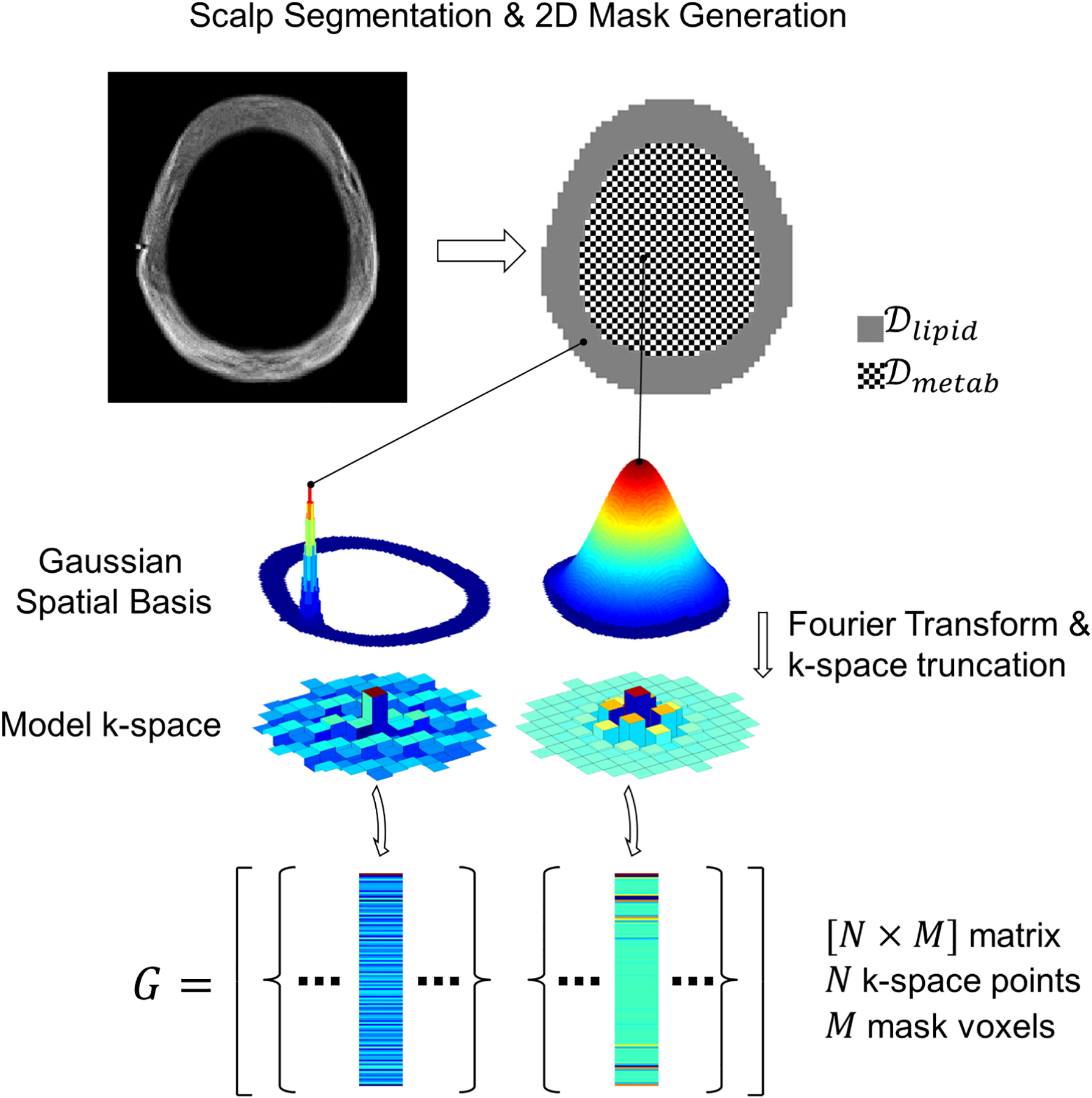
Illustration of FLIP concept for lipid removal in 2D MRSI. Scalp and brain masks are generated using multi-slice anatomical MRI (top). The scalp and brain regions are assigned different spatial smoothness defined by a Gaussian spatial function. Next, Fourier Transform and truncation are applied to the Gaussian spatial functions at each mask voxel (middle). The resulting k-space components match the MRSI acquisition. Finally, the modified k-space encoding matrix G is formed with one column for each mask voxel (bottom).

3D EPSI Methods

The FLIP, PGA, HSVD, and L2 algorithms were also demonstrated in high-resolution whole-brain 3D EPSI data. Due to the very large dimensions, the EPSI data were spatially cropped to 32×32×12 without loss of resolution, which encompassed the head including the whole cerebrum (note that the transverse resolution was larger than those in the axial plane). To reduce computer memory requirements, the lipid and metabolite region masks were partitioned into rectangular sub-regions of adjacent image pixels. FLIP and PGA on 3D EPSI used automatic scalp segmentation as the basis for the lipid and metabolite spatial masks (SPM12, Wellcome Trust Centre for Neuroimaging, UK).²⁸

Simulations

Simulations of 2D MRSI were performed to investigate lipid removal efficiency and metabolite signal leakage of the FLIP method. The regularization parameter was tested over a wide range of values from 10⁻⁹ to 10⁻³ (shown in the log scale in Fig. 2A, B). The efficiency of lipid removal and metabolite signal immunity to leakage were calculated as ratios of output and input signal root mean square values averaged over the voxels inside the brain, expressed in percentage. Metabolite input signals were defined as Gaussian spatial functions with the radial parameter of 25 cm as in Eq. 6, and the same radial parameter was used for the reconstruction.

Figure 2.

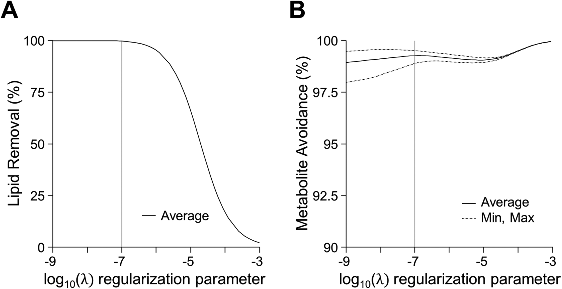
Simulation showing the effect of the regularization parameter on the lipid reconstruction characteristics. The regularization parameter can be optimized to balance between lipid removal efficiency (A) and metabolite avoidance (B). Regularization shown on a log scale revealed that a value of 10⁻⁷ was suitable for both high efficiency of lipid removal and acceptable metabolite avoidance.

HSVD, PGA and L2 implementations

The HSVD, PGA, and L2 algorithms were implemented according to published methods^4,7,29 using Matlab. HSVD requires the selection of the appropriate number of poles (K). We found that K = 6 was sufficient to reconstruct lipid spectra reliably while avoiding poles in the main metabolite region (>1.9 ppm); poles returned by HSVD outside the lipid frequency range (<1.9 ppm) were discarded from the reconstruction. HSVD was performed with K = 6 and L = 100, where L is the matrix column dimension for SVD. PGA parameters were optimized by testing the number of iterations (N_pg = 5, 10, 15, 30, 50) and image mask resolution (64, 128, and 256 base sizes). N_pg of 15 provided reliable lipid removal in PGA (2D MRSI). For 3D EPSI, N_pg was set by inspection, and while N_pg of 15 performed acceptably, N_pg of 30 provided more robust lipid removal performance and was used as a conservative specification. The same lipid segmentation was used for both FLIP and PGA.

L2 algorithm code was available from the authors (www.nmr.mgh.harvard.edu/~berkin/software.html), and the code was modified with automatic calibration of the regularization parameter (β). The β setting was adjusted for each receiver coil to reach a target of 1% and 16% residual power for 2D MRSI and 3D EPSI, respectively. The residual power levels differed due to differences in lipid signal strength per voxel in 2D MRSI and 3D EPSI data. The setup of L2 also included pre-selecting the number of voxels to include in the lipid basis, which was set by inspection as N_{lipid_basis}=10 for 2D MRSI and N_{lipid_basis}=30 for 3D EPSI with per-coil MRSI processing. All reported results for L2 utilized automatic parameter calibration.

Time Tests

Processing speeds were measured using a dedicated workstation (Windows 10, dual Intel Xeon 3GHz 6-core processors). For all 2D MRSI time tests, two trials were run for each measurement and the minimum processing time is reported. The time allocations for major operations in FLIP, PGA, and HSVD are reported as given by the Matlab code profiling tool. The measured run time of L2 includes voxel masking steps, and for 2D MRSI we report the minimum time ignoring calibration of β.

Spectral Fitting & Statistics

Spectral fitting was performed on all MRSI voxels within the head using LCModel³⁰. The spectral basis set was simulated using the VeSPA package (https://scion.duhs.duke.edu/vespa/). Concentrations of NAA, creatine (Cr), total choline (tCho), glutamate+glutamine (Glx), and myo-inositol (mI) were determined based on the internal reference method using unsuppressed water signals, without corrections for relaxation effects or tissue water concentrations. Cramer Rao Lower Bound (CRLB), linewidth, and the signal-to-noise ratio (SNR) reported by LCModel were used to evaluate the quality of data at each voxel. Spectra were considered acceptable with linewidth<0.1 ppm, SNR>3³¹, and CRLB of NAA≤20%. CRLB of NAA was chosen among those of other metabolites as a quality criterion because of the high likelihood of interference from residual lipid signals after applying each algorithm, due to its proximity to the major lipid signals at 1.3 ppm. Metabolite concentration and concentration ratios-to-creatine were reported as mean ± SD averaged over subjects. Two-tailed paired t-tests were used to compare concentrations between algorithms. The coefficient of variation (CoV) of NAA/Cr was calculated from a large number of voxels in each subject for 3D EPSI data to quantify distribution differences of NAA/Cr among algorithms. The voxel averaging process for each subject used only those voxels that passed criteria with all algorithms, i.e., the intersection of good voxels among algorithms.

Results

Simulation outcomes in Fig. 2 demonstrate the effects of lipid removal by FLIP on metabolite signals in MRSI. An optimal regularization value (λ) yielded effective lipid removal without adverse metabolite signal leakage to the lipid compartment (Fig. 2A, 2B). The metabolite signal immunity to leakage depends on the spatial width (i.e., input uniformity) and the location of input signals in the image.

In Full FOV 2D MRSI without lipid removal, dominant lipid signals were observed as expected throughout the entire head including the center of the brain (Fig. 3, top). Lipid signals originating from the scalp were reliably estimated using FLIP (Fig. 3, bottom). Upon removal of the brain as well as the edge of the brain close to the scalp (Fig. 4A) with consistent and reliable performance among 18 subjects. From a total of 1956 input spectra across all 18 subjects the FLIP, PGA, HSVD, and L2 methods yielded 90%, 57%, 29%, and 42% acceptable spectra, respectively, based on the quality criteria for SNR, linewidth, and CRLB of NAA (Table 1). Within the voxels that were well fitted by all algorithms (commonly good voxels), the mean and SD of metabolite concentration ratios-to-creatine were similar across all four methods (Table 1) although PGA showed some differences in the mean. Independently, FLIP fitting results showed the smallest variation overall while HSVD showed the greatest variability (Fig. 4B). FLIP was more consistent than PGA, HSVD, and L2, as indicated by the fewer outliers and better spatial homogeneity of maps (Supporting Figure S3).

Figure 3.

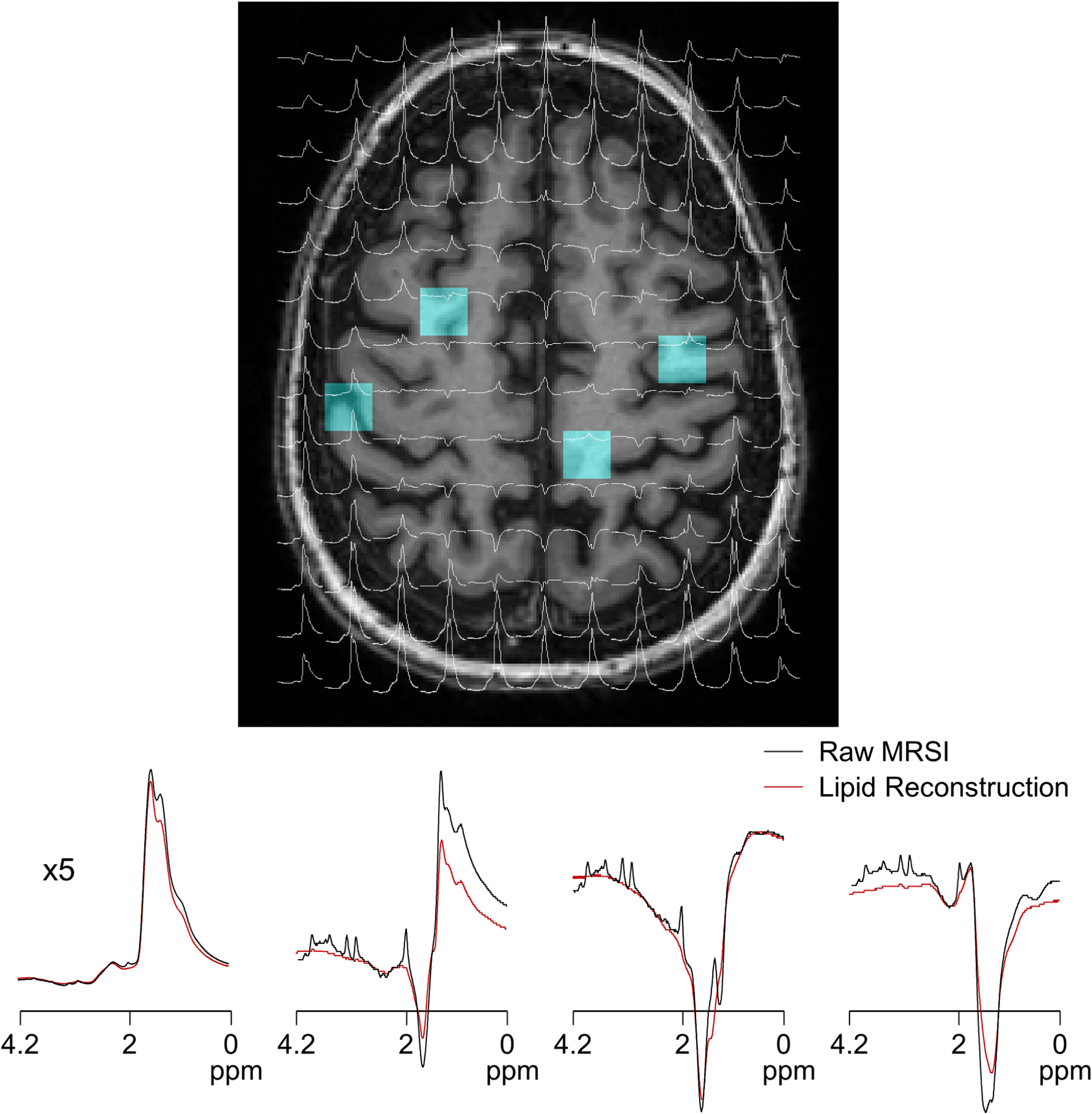
MRSI raw spectra are displayed in overlays on T1-weighted MRI (top) along with raw MRSI and extracted lipid data processed by the proposed FLIP algorithm (bottom). The spectral ranges shown are [0, 4.2] ppm. Selected central and edge voxel spectra positions are indicated by blue voxels in the MRI image (A). Raw spectra are shown in black, and reconstructed lipid spectra are overlaid in red (B). The scalp-adjacent spectrum (left) is shown at a 1/5x scale to accommodate the full amplitude of high lipid signals. The amplitudes of lipids were about 15x and 120x greater than those of creatine in the center and edge voxels, respectively.

Figure 4.

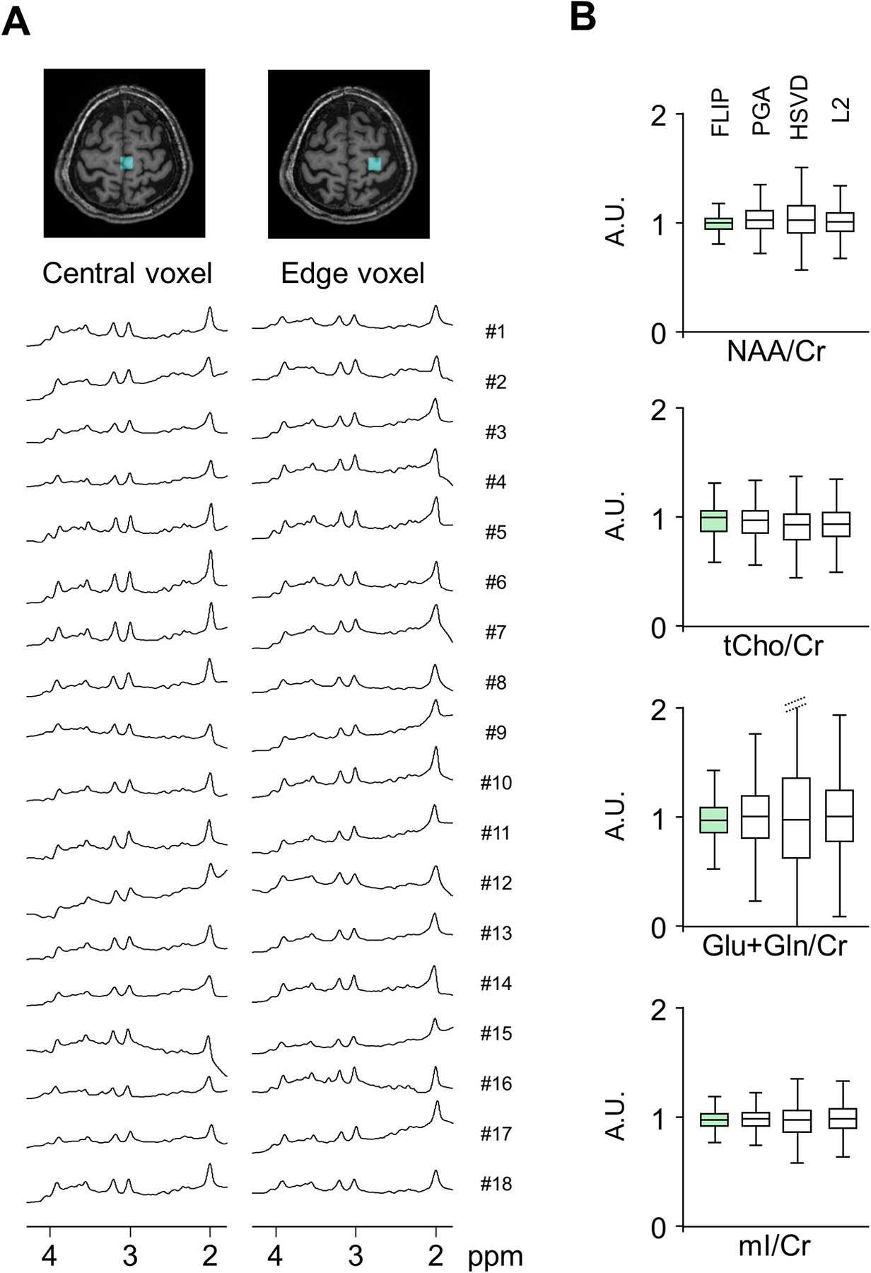
Consistency of lipid removal by FLIP. Example spectra from 18 subjects processed by the proposed lipid removal technique, showing central and edge voxels (A). The proposed method yielded reliably clear metabolite spectra with little residual lipid baselines in all 18 subjects. All spectra were processed using 1.0 Hz Lorentzian line broadening, 0.2 Gaussian broadening, and 0^th order phase correction. Group analysis (N=18) of metabolite concentration ratios-to-creatine, normalized by those of FLIP processed data are shown for each processing method (B). Only voxels satisfying the quality criteria of linewidth<0.1 ppm, SNR>3, and CRLB of NAA≤20% were included in the analysis.

Table 1.

Performance comparisons of algorithms in 2D full-FOV MRSI

Algorithms	Processing timea (s)	Statistics by voxel		Statistics by subjectc
		No. of voxels passed quality criteriab	Mean NAA CRLB	NAA/Cr	tCho/Cr	Glx/Cr	mI/Cr
FLIP	8	1752 (90%)	5.7	1.56 ± 0.08	0.27 ± 0.02	1.72 ± 0.12	0.82 ± 0.12
PGA	32	1108 (57%)	5.7	1.63 ± 0.09*	0.26 ± 0.02***	1.79 ± 0.20*	0.76 ± 0.11***
HSVD	107	571 (29%)	7.9	1.56 ± 0.09	0.26 ± 0.02	1.71 ± 0.17	0.78 ± 0.11**
L2	9	818 (42%)	7.9	1.56 ± 0.13	0.27 ± 0.02	1.73 ± 0.17	0.79 ± 0.11*

^aImage size = 64×64. PGA was performed with N_pg= 15 and HSVD with L=100.

^bMRS data quality criteria: linewidth<0.1 ppm, SNR>3, and CRLB of NAA<20%.

^cMetabolite concentrations in each subject were calculated from the central voxels that passed quality criteria in all algorithms.

^*:p < 0.05;

^**:p < 0.01;

^***:p < 0.001 based on paired two-tailed t-test in comparison with FLIP outcomes.

Note: All values are shown in mean ± SD.

Metabolite quantification results were compared between restricted VOI MRSI and full FOV MRSI with lipid removal by FLIP, PGA, HSVD, and L2 processing using the data acquired consecutively from the same subject (Fig. 5). The concentrations for 25 voxels (5×5 white square in Fig. 5A) within the VOI of restricted VOI MRSI scan are used as a reference for comparison. Mean metabolite to Cr concentration ratios are shown for the central 5×5 and 7×7 voxels for all four algorithms in the order of FLIP, PGA, HSVD, and L2 (Fig. 5B). The concentration ratios were similar in 5×5 and 7×7 voxels across all four algorithms. However, the variance of FLIP was the lowest and HSVD the highest, consistent with the data from 18 subjects in Fig. 4. Mean metabolite concentrations of full FOV MRSI within the central 5×5 voxels were similar to those from restricted VOI MRSI for FLIP and PGA, while those from HSVD and L2 showed some reduction of concentration values and HSVD showed greater variance (Fig. 5C). Each algorithm was further evaluated by examining the pointwise subtraction of reference spectra (restricted VOI MRSI) from full FOV MRSI spectra processed with each algorithm. The difference spectra processed with FLIP (Δ FLIP in Supporting Figure S1) were consistently flatter in comparison with those processed with PGA, HSVD, and L2, indicating excellent lipid removal performance of FLIP. HSVD showed the largest variability, while the L2 results showed underestimation of the mean concentrations of NAA, Cr, and Glx.

Figure 5.

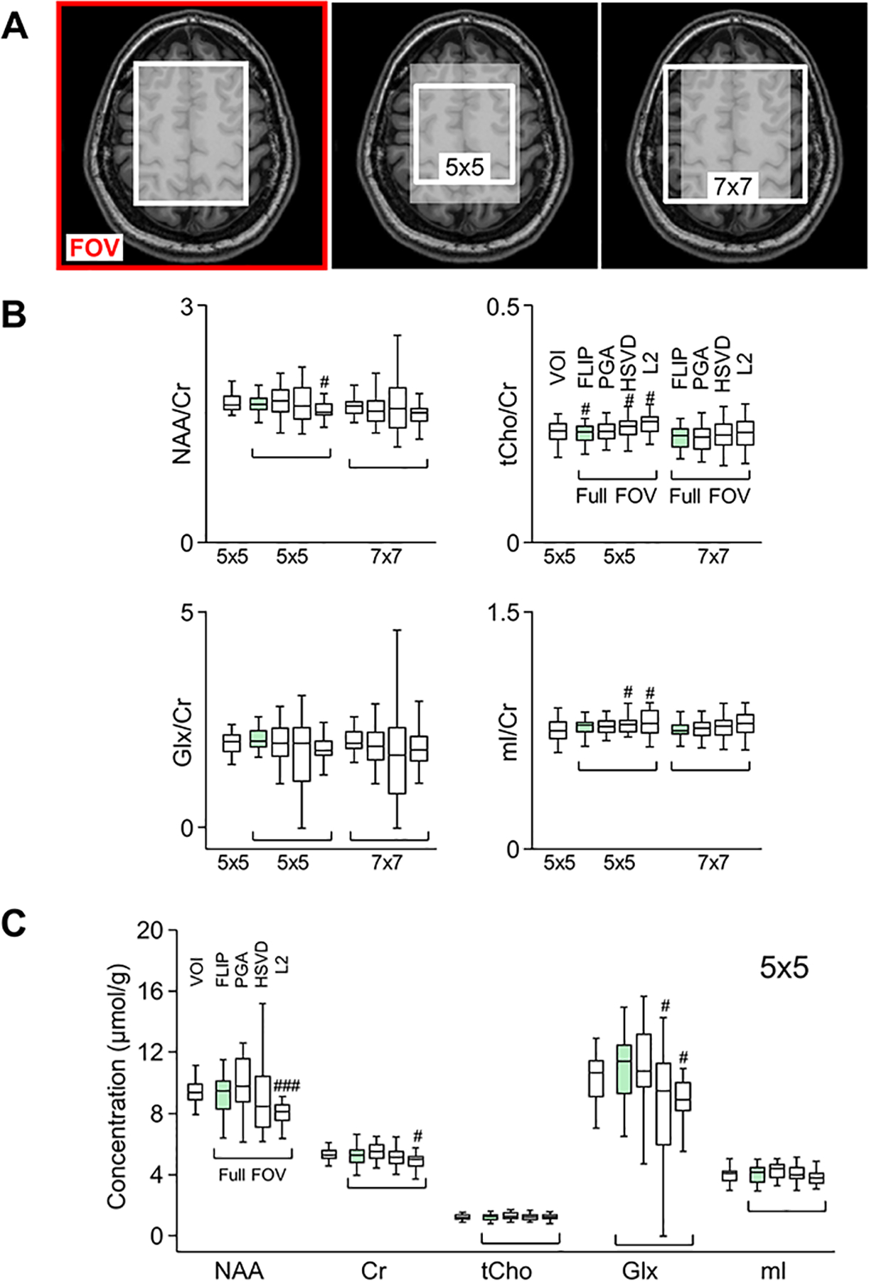
Performance of lipid removal algorithms (FLIP, PGA, HSVD, and L2) with full FOV MRSI in comparison with restricted VOI MRSI. The central white region (A, left) shows the nominal VOI used for restricted VOI MRSI. The white boxes in MRI (A, middle and right) indicate 5×5 and 7×7 voxel regions used to obtain average metabolite concentrations. All voxels within 5×5 and 7×7 regions were included in data analysis of metabolite-to-creatine ratios (B) or absolute concentrations (C). Box plots show 25 percentile, median, 75 percentile, and extreme values. Mean and variance of metabolite concentrations and their ratios-to-creatine are compared among algorithms in reference to restricted VOI MRSI for the 5×5 region. #: p<0.05; ### p<0.001 with two-tailed paired t-test between concentrations of each voxel from each algorithm and those from VOI (n=25 voxels).

Finally, the performance of FLIP was evaluated in one of the most challenging conditions for lipid removal, the combination of short TE of 16 ms and no lipid suppression in a high-resolution whole-brain 3D EPSI data set (Fig. 6). The performance of FLIP for lipid removal of 3D EPSI was similar to that of 2D MRSI, as demonstrated by consistent spectral patterns in various brain regions, e.g., GM, WM, and the subcortical area (Fig. 6A, top). Metabolite maps showed a clear contrast between GM and WM, especially in the Cr concentration maps, and excellent volume coverage including the cortical regions near the edge of the brain. When compared with PGA, HSVD, and L2, FLIP processing provided more robust lipid removal performance as shown in Fig. 6B–D and Table 2, as demonstrated by fewer outlier voxels for NAA/Cr and by lower CRLB values. The number of successfully fitted voxels were 38,443 (FLIP), 31,846 (PGA), 29,241 (HSVD) and 31,676 (L2). FLIP yielded 28%, 37%, and 31% more good quality voxels than PGA, HSVD, and L2, respectively (Table 2). The distribution of NAA/Cr values in the whole brain was narrower in FLIP than in PGA, HSVD, and L2 (Fig. 6B), and similarly, the CRLB of NAA was lower in FLIP, indicating better spectral fitting, i.e., less lipid contamination. FLIP spectra showed excellent lipid removal performance with no visible adverse metabolite signal losses (See Supporting Figure S4.).

Figure 6.

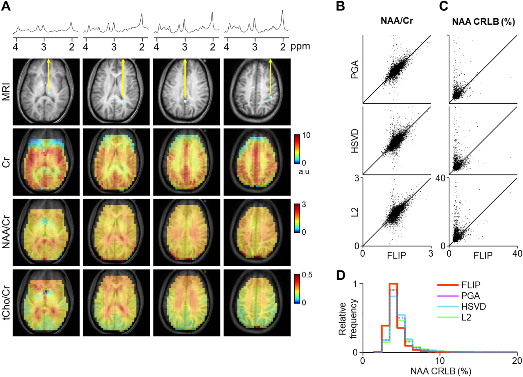
Representative spectra and quantitative metabolite maps of high-resolution whole-brain 3D EPSI are shown after lipid removal using FLIP implementation (A). Quantification results of 3D EPSI data are shown from 10 subjects, using FLIP and PGA (B-E). Metabolite maps are shown from four transverse slices of whole-brain 3D EPSI, including the thalamus, white matter, and gray matter. FLIP processing was performed at the native reconstructed EPSI resolution, and k-space apodization was applied prior to spectral fitting with a 1.3 cm effective width (FWHM). Artifacts and dropouts in the anterior region are likely due to the effect of B0 inhomogeneity near the sinus cavity. Scatter plots show (B) NAA/Cr and (C) NAA CRLB (%) with lipid removal by FLIP and PGA. The NAA/Cr and NAA CRLB (%) values are also summarized by histograms (D, E). Results using PGA lipid removal showed a broader spread of NAA/Cr values, suggesting worse quantitative accuracy compared with FLIP. The PGA CRLB values showed worse spectral fitting outcomes than FLIP. Spectral fitting was performed using LCModel on 13,084 voxels. Central four slices of 3D EPSI data were used from each subject, and voxels were restricted to both PGA and FLIP results that have passed the criteria of tissue fraction > 0.5 and linewidth < 0.1 ppm. Voxels with zero concentration have been excluded.

Table 2.

Performance comparisons of algorithms in 3D EPSI.

Algorithms	Processing timea (min)	Statistics by voxel		Statistics by subjectd
		No. of voxels with NAA CRLB ≤ 20%b	No. of voxels passed quality criteriac	NAA/Cr	CoV of NAA/Cre	Median NAA CRLBf
FLIP	41	36,829 (96%)	30,595 (80%)	1.44 ± 0.079	0.023 ± 0.006	4.16 ± 0.44
PGA	79	28,823 (91%)	23,827 (75%)	1.46 ± 0.084	0.030 ± 0.007*	4.50 ± 0.41**
HSVD	10	26,318 (90%)	22,260 (76%)	1.45 ± 0.082	0.033 ± 0.005***	4.56 ± 0.33**
L2	1.4	27,615 (87%)	23,353 (74%)	1.47 ± 0.083	0.035 ± 0.006***	4.60 ± 0.41***

^aImage size = 64×64×32. PGA was performed with N_pg= 30.

^bPercentages are calculated from successfully fitted voxels using the LCModel in each algorithm (FLIP: 38,443; PGA: 31,846; HSVD: 29,241; L2: 31,676 voxels).

^cMRS data quality criteria: linewidth < 0.1 ppm, CRLB of NAA ≤ 20% and tissue fraction > 50%.

^dSubject-based processing was performed using the voxels that passed the MRS data quality criteria in all algorithms (mutual good voxels).

^eCoefficient of variation (CoV) of NAA/Cr was calculated as (standard deviation of NAA/Cr) divided by (mean of NAA/Cr) in each subject.

^fMedian of NAA CRLB value was calculated from the distribution of NAA CRLB values from the central five slices of 3D EPSI data in each subject, with individual quality criteria (not mutual good voxels).

^*:p < 0.05;

^**:p < 0.01;

^***:p < 0.001 based on paired two-tailed t-test in comparison with FLIP outcomes.

Note: All values are shown in mean ± SD.

The processing time of FLIP lipid removal in 2D MRSI was 8 s (64×64 image base size and 49 k-space points), which was significantly shorter than 32 s for PGA (N_pg= 15 and image base size 64×64), 107 s for HSVD (L=100) and similar to the 9 s required for L2 (Fig. 7A, Table 1). The measured run time of L2 included mask preparation steps but did not include iterative adjustment of the β parameter. The dependence of processing time on image matrix size for FLIP and PGA is shown in Figs. 7A–C, including the dependence of iterations in PGA (Fig. 7C) and the number of spectral points in HSVD (Fig. 7D). Overall, FLIP was faster than the other algorithms for the image base size up to about 176×176. PGA processing spent 48% of total processing time in FFT and inverse FFT, 44% in other mathematical operations (not FFT-shift), and the remainder in other overhead. HSVD processing spent 90% of total time in computing SVD. FLIP processing in 2D MRSI spent 62% of total time to calculate the spatial encoding matrix (G), 23% in SVD and regularized pseudoinverse calculation, and the remainder in the final matrix multiplication and other overhead when tested at 128 base image size.

Figure 7.

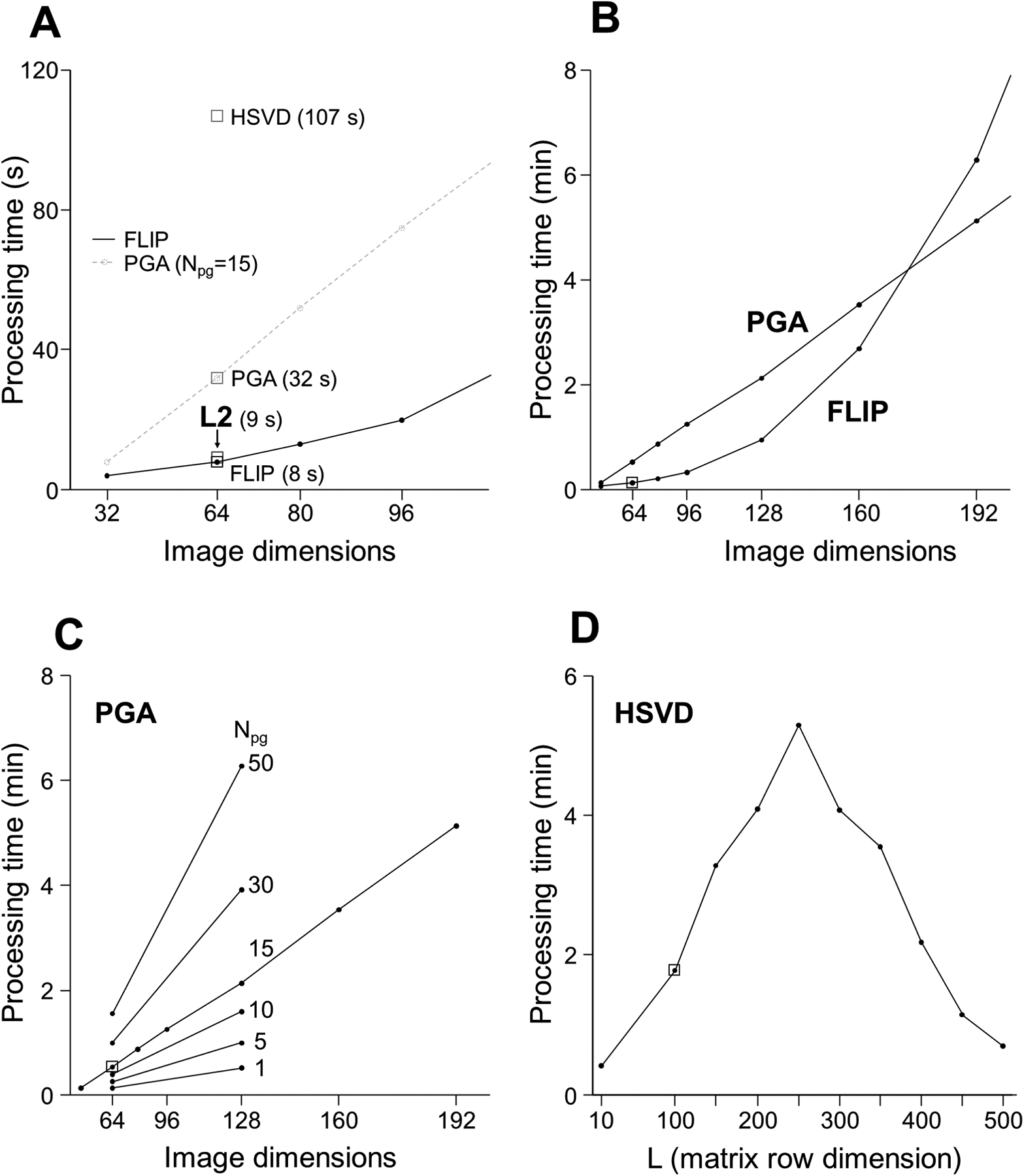
Processing time for the FLIP, PGA, HSVD, and L2 algorithms. Small squares indicate the parameters for the fastest processing speed at the best lipid removal efficacy at a given condition (A). FLIP and PGA are parameterized by a base image dimension, equal to the square root of the 2D image size. HSVD was parameterized by the matrix column dimension. The FLIP time was the fastest and depended on a mix of FFT, SVD, and other operations. With high image dimensions greater than ~170, PGA became faster than FLIP (B). The PGA processing time was proportional to the number of iterations as expected (C). The HSVD peak processing time coincided with a maximal, square matrix size (D). The L2 processing time includes preparation steps comparable with portions of the other algorithms, minus additional time used for per-subject parameter calibration. The measured processing times demonstrate a significant speed advantage of the FLIP algorithm.

The FLIP processing time for 3D EPSI was between 30 to 41 min, depending on the matrix column dimension (11,000 to 15,000 depending on the lipid and metabolite mask sizes). The row dimension was fixed as the k-space size of 12,288 points (32×32×12). The PGA processing time was 40 to 80 minutes (Npg=15 and 30, respectively), while HSVD required 10 minutes and L2 took just 1.4 minutes including automatic parameter calibration. The relatively small basis size of L2 led to a very fast speed, however, it yielded fewer good quality voxels.

Discussion

We have presented a new lipid removal method that takes advantage of precise scalp lipid segmentation from high-resolution MRI to inform a spatial model of signals in MRSI. The model used Gaussian apodization to approximate k-space patterns of lipid and metabolite inputs. This method could provide fast and robust reconstruction and removal of lipid signals through a regularized least-squares approach. FLIP demonstrated effective and efficient isolation and removal of strong lipid signal contamination in full FOV MRSI originating from the scalp. This opens the possibility of accessing cortical areas of the brain with the capability of lipid removal from full FOV MRSI. The ability to measure metabolic alterations in the cortical areas is important in various neurological disorders, e.g., Alzheimer’s disease and related disorders. However, most MRS measurements are currently performed on the rectangular VOI excluding the cortical areas due to its proximity to the scalp, which poses substantial technical challenges, especially in handling interference from strong lipid signals. Although the major advantage of FLIP can be appreciated in full FOV MRSI, it could also be reliably applied to restricted VOI MRSI to improve incomplete lipid removal using VOI selection, OVS, and/or inversion lipid nulling.

In 2D MRSI, full FOV and restricted VOI MRSI comparisons demonstrated that FLIP showed the closest concentration values to those of the restricted VOI MRSI within the VOI (5×5) and the least concentration variations among the four algorithms. This suggests that FLIP processing could more effectively remove interfering lipid signals without adversely affecting spectral quantification compared with other algorithms. With 18 subject data, FLIP yielded significantly more voxels that passed the quality criteria and showed fewer variations of concentration values than others, demonstrating the robustness of FLIP. In 3D EPSI data, FLIP showed similar effectiveness and robustness of lipid removal as in 2D MRSI data, providing a larger number of voxels with accepted spectral quality and fewer variations in concentration than other algorithms. Performance differences between algorithms could be better represented by the number of voxels with accepted spectral quality and concentration variations than the mean concentration values that were similar among algorithms. Similar mean concentrations among algorithms could be explained by the effect of averaging in the large number of voxels.

Worse performance of HSVD could be attributed to over- or under-fitting with an incorrect number of poles. Overfitting is problematic in HSVD because the next most significant pole is often a metabolite singlet or macromolecule feature, resulting in its complete removal. The performance of PGA was generally better than HSVD but inferior to FLIP. While performing well in ideal conditions, PGA could suffer from its sensitivity to inaccuracies of positional alignment between MRI and MRSI or lipid mask shapes, or insufficient k-space sizes in MRSI. Additionally, unlike FLIP, PGA does not allow any adjustable parameters to increase its lipid removal capacity. L2 might have been negatively affected by overfitting of signals including some attenuation of metabolites (Fig. 5C), which could be mitigated by increasing the targeted residual lipid power, using fewer basis spectra, or changing the selected basis voxels. While the performance of L2 is sensitive to implementation details including the setup and calibration approaches, those details have not been standardized to our knowledge. In our implementation of L2, we specified one choice of regularization per coil with a fixed basis size and selection process. We observed, in some cases, when L2 was adjusted to remove the most lipid signals possible, the residual spurious artifacts could become similar in amplitude and linewidth to metabolites such as NAA. Therefore, moderate choices of basis size and suppression level were necessary.

FLIP was the fastest algorithm for 2D MRSI compared with PGA, HSVD, and L2 (Table 1). Processing speeds depend on various factors including the number of floating-point operation (flop) counts of the algorithm, the CPU frequency, and system-dependent optimizations of subroutines such as FFT (FFTW^32,33), matrix multiplication, and SVD (BLAS and LAPACK^34,35). PGA required 10 to 50 image-sized FFTs for each chemical shift point. HSVD involves the SVD of many small matrices, and it is independent of MRI image dimensions. L2 was slowed by the need to iteratively adjust towards the target lipid residual level, although we note that it might be sped up with a better implementation. In 3D EPSI data sets, FLIP was slower than HSVD and L2 but faster than PGA. The speed gain of HSVD and L2 is partially due to processing only the intracranial voxels rather than running over the entire volume. The extremely fast L2 speed may have come at the expense of performance because L2 showed less robust results than FLIP. More sophisticated optimization could have improved L2 at a cost of slower processing. The speed penalty in FLIP was due to large matrix inverse operations for 3D EPSI data. While it was feasible to perform such operations, they required significantly increased computation time. In the current FLIP implementation for 3D EPSI data, we focused on optimizing lipid removal performance and overlooked the impracticality of the large matrix inversion. Possible approaches to speed up FLIP are through spatial or dimensional restrictions, as done implicitly with the voxel selection by the coil in L2. Alternatively, if FLIP was performed in 2D mode, i.e., slice-by-slice processing, as in the 2D data, the speed could be comparable to L2.

The fast processing speed of FLIP in 2D mode offers some new opportunities in MRSI. While the total computation time of the proposed algorithm was around 8 seconds for the 2D MRSI application, the final data application step could be repeated much faster, in as little as a fraction of a second. This presents an opportunity for rapid MRI-MRSI spatial alignment optimization and parameter tuning that would be prohibitive with much slower methods. We observed small spatial MRI-MRSI misalignment (mostly less than 5 mm translation) in healthy older adults. Based on the analysis using 130 data sets, a mismatch by 5 mm resulted in about 0.5% lipid removal efficiency reduction, which could significantly impact spectral quality in the areas with large lipid signals, e.g., edge of the brain. When greater mismatches are expected in a more challenging subject population (e.g., children and patients with Alzheimer’s disease or movement disorders), the ability to optimize the alignment using FLIP could be particularly helpful in maintaining the accuracy of metabolic imaging outcomes. Since the FLIP implementation requires only anatomical MRI and MRSI raw data that are typically included in MRSI scans, FLIP could be straightforwardly added into existing MRSI processing routines. FLIP performed adequately on a wide range of lipid tissue thickness, from very thin to exceptionally thick (upwards of 10 mm) as shown in Supporting Figure S2, using a single set of parameters, demonstrating the generality of the k-space regression concept in FLIP.

Because FLIP is solely based on spatial information, it could be useful for clinical applications that present brain lipids as an important pathological feature. Moreover, macromolecules could be better revealed by reducing lipid contamination. We note, however, that FLIP did not eliminate the contribution of scalp lipid signals to the brain voxels. The imperfections in removing residual lipid spectral components could be attributed to limited k-space size, spatial mismatch due to subject motion during scans, and a relatively thick MRSI slab that creates a non-separable scalp and brain overlap in 2D. These challenges could be mitigated by using a sufficiently thin slab in 2D MRSI, 3D high-resolution MRSI (e.g., EPSI),^25,26,36 and real-time motion correction methods.³⁷

This study demonstrates the robust and effective lipid removal of FLIP in a 3D EPSI data set at short TE without the use of any lipid suppression schemes. In general, whole-brain 3D EPSI data are acquired using inversion recovery for lipid nulling at a long TE (≥ 50 ms) to reduce the effect of lipid artifacts, and then lipid signals are further removed using post-processing lipid removal algorithms (e.g., PGA). However, short TE is desirable for brain MRSI to obtain higher SNR for reliable quantification of a large number of metabolites. The use of inversion recovery for lipid nulling also reduces SNR. Therefore, considering improved lipid removal performance of FLIP over commonly used PGA, FLIP promises the feasibility of whole-brain 3D EPSI with short TE and improved SNR for clinical applications. Since 3D EPSI posed significant challenges regarding computer memory and processing time requirements due to the large MRSI data matrix size compared to 2D MRSI, further work is necessary to realize the full potential of FLIP in high-resolution whole-brain MRSI with the full basis sets through an optimized computation strategy.

In summary, we have demonstrated an effective new method for the removal of lipid signals arising from the scalp in full FOV MRSI and high-resolution whole-brain 3D EPSI solely based on spatial information. The major strengths of FLIP are its speed in 2D MRSI and effectiveness even for short TE and low-resolution MRSI that are technically challenging. Given that it uses only spatial prior information, spectral lipid or water removal could still be applied (HSVD, L2). Moreover, FLIP can be easily combined with novel MRSI reconstruction frameworks, e.g., SLIM, BASE-SLIM, SPICE, and others,^38–48 to further improve the anatomical specificity of MRSI reconstruction and spectral quality.

Supplementary Material

supinfo

Figure S1. Comparisons of spectra within the central 5×5 voxels processed with FLIP, PGA, HSVD, and L2 in reference with restricted VOI MRSI. Spectra from all 25 voxels are displayed for the restricted VOI (black), full FOV MRSI processed with FLIP (green), PGA (red), HSVD (blue), and L2 (violet) (top). Difference spectra were obtained by subtracting restricted VOI from full FOV MRSI spectra in each voxel (bottom).

Figure S2. Results of in-house automatic lipid segmentation used in the FLIP and PGA algorithms. Two subjects are displayed, showing the superior and inferior slab slices, as examples of very thin (A) and very thick (B) scalp lipids. At right, the lipid segmentation is shown by an overlay in yellow over the MRI (may not be apparent in grayscale).

Figure S3. 2D MRSI maps of SNR, linewidth (LW, ppm), and concentration ratios for NAA, Cr, tCho, Glx, and mI to creatine for 18 subjects. A total of 7,776 successfully fitted voxels are shown. Images for one subject (inset) display an expanded view of the MRSI maps with grayscale bars for the image scale used for all the data.

Figure S4. Raw spectra are shown (black) superimposed with the extracted lipid spectra (shown in red) using FLIP on whole-brain 3D EPSI data. Representative spectra are from a row of ten voxels in the sagittal direction. All voxels are shown with the same scaling factor, demonstrating large lipid signals obtained at short TE (=16 ms) without lipid suppression. The lipid removal efficiency is demonstrated by the excellent agreement among the lipid components of the raw spectra and extracted lipid spectra.

References

- 1.Ren J, Dimitrov I, Sherry AD, Malloy CR. Composition of adipose tissue and marrow fat in humans by 1H NMR at 7 Tesla. J Lipid Res. 2008;49(9):2055–2062. [DOI] [PMC free article] [PubMed] [Google Scholar]
- 2.Tkac I, Deelchand D, Dreher W, et al. Water and lipid suppression techniques for advanced 1H MRS and MRSI: Experts’ consensus recommendations. NMR Biomed. 2020;DOI: 10.1002/nbm.4459. [DOI] [PMC free article] [PubMed] [Google Scholar]
- 3.Pijnappel WWF, Vandenboogaart A, Debeer R, Vanormondt D. SVD-Based Quantification of Magnetic-Resonance Signals. Journal of Magnetic Resonance. 1992;97(1):122–134. [Google Scholar]
- 4.Barkhuijsen H, Debeer R, Vanormondt D. Improved Algorithm for Noniterative Time-Domain Model-Fitting to Exponentially Damped Magnetic-Resonance Signals. Journal of Magnetic Resonance. 1987;73(3):553–557. [Google Scholar]
- 5.Kumaresan R, Tufts DW. Estimating the Parameters of Exponentially Damped Sinusoids and Pole-Zero Modeling in Noise. Ieee Transactions on Acoustics Speech and Signal Processing. 1982;30(6):833–840. [Google Scholar]
- 6.Vanhuffel S, Chen H, Decanniere C, Vanhecke P. Algorithm for Time-Domain Nmr Data Fitting Based on Total Least-Squares. Journal of Magnetic Resonance Series A. 1994;110(2):228–237. [Google Scholar]
- 7.Haupt CI, Schuff N, Weiner MW, Maudsley AA. Removal of lipid artifacts in 1H spectroscopic imaging by data extrapolation. Magn Reson Med. 1996;35(5):678–687. [DOI] [PMC free article] [PubMed] [Google Scholar]
- 8.Tsao J Extension of finite-support extrapolation using the generalized series model for MR spectroscopic imaging. Ieee Transactions on Medical Imaging. 2001;20(11):1178–1183. [DOI] [PubMed] [Google Scholar]
- 9.Eslami R, Jacob M. Robust reconstruction of MRSI data using a sparse spectral model and high resolution MRI priors. IEEE Trans Med Imaging. 2010;29(6):1297–1309. [DOI] [PubMed] [Google Scholar]
- 10.Ma C, Lam F, Johnson CL, Liang ZP. Removal of nuisance signals from limited and sparse 1H MRSI data using a union-of-subspaces model. Magn Reson Med. 2016;75(2):488–497. [DOI] [PMC free article] [PubMed] [Google Scholar]
- 11.Dong Z, Hwang JH. Lipid signal extraction by SLIM: application to 1H MR spectroscopic imaging of human calf muscles. Magn Reson Med. 2006;55(6):1447–1453. [DOI] [PubMed] [Google Scholar]
- 12.Bilgic B, Chatnuntawech I, Fan AP, et al. Fast image reconstruction with L2-regularization. J Magn Reson Imaging. 2014;40(1):181–191. [DOI] [PMC free article] [PubMed] [Google Scholar]
- 13.Bhattacharya I, Jacob M. Compartmentalized low-rank recovery for high-resolution lipid unsuppressed MRSI. Magn Reson Med. 2016. [DOI] [PMC free article] [PubMed] [Google Scholar]
- 14.Tsai SY, Lin YR, Lin HY, Lin FH. Reduction of lipid contamination in MR spectroscopy imaging using signal space projection. Magn Reson Med. 2019;81(3):1486–1498. [DOI] [PubMed] [Google Scholar]
- 15.Tugnoli V, Tosi MR, Tinti A, Trinchero A, Bottura G, Fini G. Characterization of lipids from human brain tissues by multinuclear magnetic resonance spectroscopy. Biopolymers. 2001;62(6):297–306. [DOI] [PubMed] [Google Scholar]
- 16.Singh I, Pujol A. Pathomechanisms underlying X-adrenoleukodystrophy: a three-hit hypothesis. Brain Pathol. 2010;20(4):838–844. [DOI] [PMC free article] [PubMed] [Google Scholar]
- 17.Golub GH, Van Loan CF. Matrix computations. Fourth edition. ed. Baltimore: The Johns Hopkins University Press; 2013. [Google Scholar]
- 18.Matej S, Lewitt RM. Efficient 3D Grids for Image-Reconstruction Using Spherically-Symmetrical Volume Elements. Ieee Transactions on Nuclear Science. 1995;42(4):1361–1370. [Google Scholar]
- 19.Matej S, Lewitt RM. Practical considerations for 3-D image reconstruction using spherically symmetric volume elements. IEEE Trans Med Imaging. 1996;15(1):68–78. [DOI] [PubMed] [Google Scholar]
- 20.Marabini R, Herman GT, Carazo JM. 3D reconstruction in electron microscopy using ART with smooth spherically symmetric volume elements (blobs). Ultramicroscopy. 1998;72(1–2):53–65. [DOI] [PubMed] [Google Scholar]
- 21.Trampert P, Vogelgesang J, Schorr C, et al. Spherically symmetric volume elements as basis functions for image reconstructions in computed laminography. J Xray Sci Technol. 2017. [DOI] [PubMed] [Google Scholar]
- 22.Tikhonov AN. Ill-Posed Problems of Linear Algebra and a Stable Method for Their Solution. Doklady Akademii Nauk Sssr. 1965;163(3):591–&. [Google Scholar]
- 23.Scheenen TW, Klomp DW, Wijnen JP, Heerschap A. Short echo time 1H-MRSI of the human brain at 3T with minimal chemical shift displacement errors using adiabatic refocusing pulses. Magn Reson Med. 2008;59(1):1–6. [DOI] [PubMed] [Google Scholar]
- 24.Lee CY, Choi IY, Lee P. Prospective frequency correction using outer volume suppression-localized navigator for MR spectroscopy and spectroscopic imaging. Magn Reson Med. 2018. [DOI] [PMC free article] [PubMed] [Google Scholar]
- 25.Maudsley AA, Domenig C, Govind V, et al. Mapping of brain metabolite distributions by volumetric proton MR spectroscopic imaging (MRSI). Magn Reson Med. 2009;61(3):548–559. [DOI] [PMC free article] [PubMed] [Google Scholar]
- 26.Ebel A, Maudsley AA. Improved spectral quality for 3D MR spectroscopic imaging using a high spatial resolution acquisition strategy. Magn Reson Imaging. 2003;21(2):113–120. [DOI] [PubMed] [Google Scholar]
- 27.Bydder M, Larkman DJ, Hajnal JV. Combination of signals from array coils using image-based estimation of coil sensitivity profiles. Magnetic resonance in medicine : official journal of the Society of Magnetic Resonance in Medicine / Society of Magnetic Resonance in Medicine. 2002;47(3):539–548. [DOI] [PubMed] [Google Scholar]
- 28.Ashburner J, Friston KJ. Unified segmentation. Neuroimage. 2005;26(3):839–851. [DOI] [PubMed] [Google Scholar]
- 29.Papoulis A New Algorithm in Spectral Analysis and Band-Limited Extrapolation. Ieee Transactions on Circuits and Systems. 1975;22(9):735–742. [Google Scholar]
- 30.Provencher SW. Automatic quantitation of localized in vivo 1H spectra with LCModel. NMR Biomed. 2001;14(4):260–264. [DOI] [PubMed] [Google Scholar]
- 31.Wilson M, Andronesi O, Barker PB, et al. Methodological consensus on clinical proton MRS of the brain: Review and recommendations. Magn Reson Med. 2019;82(2):527–550. [DOI] [PMC free article] [PubMed] [Google Scholar]
- 32.Frigo M, Johnson SG. FFTW: an adaptive software architecture for the FFT. Paper presented at: Acoustics, Speech and Signal Processing, 1998. Proceedings of the 1998 IEEE International Conference on; 12–15 May 1998, 1998. [Google Scholar]
- 33.Frigo M, Johnson SG. The design and implementation of FFTW3. Proceedings of the Ieee. 2005;93(2):216–231. [Google Scholar]
- 34.Blackford LS, Demmel J, Dongarra J, et al. An updated set of Basic Linear Algebra Subprograms (BLAS). Acm Transactions on Mathematical Software. 2002;28(2):135–151. [Google Scholar]
- 35.Anderson E, Bai Z, Bischof C, et al. LAPACK Users’ Guide. Society for Industrial and Applied Mathematics; 1999. [Google Scholar]
- 36.Wiedermann D, Schuff N, Matson GB, et al. Short echo time multislice proton magnetic resonance spectroscopic imaging in human brain: metabolite distributions and reliability. Magn Reson Imaging. 2001;19(8):1073–1080. [DOI] [PubMed] [Google Scholar]
- 37.Andronesi OC, Bhattacharyya PK, Bogner W, et al. Frequency and motion correction techniques for magnetic resonance spectroscopy: Experts’ consensus recommendations. NMR Biomed. 2020;DOI: 10.1002/nbm.4364. [DOI] [Google Scholar]
- 38.Adany P, Choi I-Y, Lee P. B0-adjusted and sensitivity-encoded spectral localization by imaging (BASE-SLIM) in the human brain in vivo. NeuroImage. 2016;134:355–364. [DOI] [PMC free article] [PubMed] [Google Scholar]
- 39.Hu X, Levin DN, Lauterbur PC, Spraggins T. SLIM: spectral localization by imaging. Magn Reson Med. 1988;8(3):314–322. [DOI] [PubMed] [Google Scholar]
- 40.Liang ZP, Lauterbur PC. A generalized series approach to MR spectroscopic imaging. IEEE Trans Med Imaging. 1991;10(2):132–137. [DOI] [PubMed] [Google Scholar]
- 41.von Kienlin M, Mejia R. Spectral Localization with Optimal Pointspread Function. Journal of Magnetic Resonance. 1991;94(2):268–287. [Google Scholar]
- 42.Tsao J, Behnia B, Webb AG. Unifying linear prior-information-driven methods for accelerated image acquisition. Magn Reson Med. 2001;46(4):652–660. [DOI] [PubMed] [Google Scholar]
- 43.von Kienlin M, Beer M, Greiser A, et al. Advances in human cardiac P-31-MR spectroscopy: SLOOP and clinical applications. Journal of Magnetic Resonance Imaging. 2001;13(4):521–527. [DOI] [PubMed] [Google Scholar]
- 44.Bashir A, Yablonskiy DA. Natural linewidth chemical shift imaging (NL-CSI). Magn Reson Med. 2006;56(1):7–18. [DOI] [PMC free article] [PubMed] [Google Scholar]
- 45.Khalidov I, Van De Ville D, Jacob M, Lazeyras F, Unser M. BSLIM: spectral localization by imaging with explicit B0 field inhomogeneity compensation. IEEE Trans Med Imaging. 2007;26(7):990–1000. [DOI] [PubMed] [Google Scholar]
- 46.An L, Warach S, Shen J. Spectral localization by imaging using multielement receiver coils. Magn Reson Med. 2011;66(1):1–10. [DOI] [PMC free article] [PubMed] [Google Scholar]
- 47.Zhang Y, Gabr RE, Zhou J, Weiss RG, Bottomley PA. Highly-accelerated quantitative 2D and 3D localized spectroscopy with linear algebraic modeling (SLAM) and sensitivity encoding. J Magn Reson. 2013;237:125–138. [DOI] [PMC free article] [PubMed] [Google Scholar]
- 48.Ma C, Lam F, Ning Q, Johnson CL, Liang ZP. High-resolution (1) H-MRSI of the brain using short-TE SPICE. Magn Reson Med. 2017;77(2):467–479. [DOI] [PMC free article] [PubMed] [Google Scholar]
Associated Data
This section collects any data citations, data availability statements, or supplementary materials included in this article.
Supplementary Materials