Global Sensitivity Analysis with Mixtures: A Generalized Functional ANOVA Approach

Abstract

This work investigates aspects of the global sensitivity analysis of computer codes when alternative plausible distributions for the model inputs are available to the analyst. Analysts may decide to explore results under each distribution or to aggregate the distributions, assigning, for instance, a mixture. In the first case, we lose uniqueness of the sensitivity measures, and in the second case, we lose independence even if the model inputs are independent under each of the assigned distributions. Removing the unique distribution assumption impacts the mathematical properties at the basis of variance‐based sensitivity analysis and has consequences on result interpretation as well. We analyze in detail the technical aspects. From this investigation, we derive corresponding recommendations for the risk analyst. We show that an approach based on the generalized functional ANOVA expansion remains theoretically grounded in the presence of a mixture distribution. Numerically, we base the construction of the generalized function ANOVA effects on the diffeomorphic modulation under observable response preserving homotopy regression. Our application addresses the calculation of variance‐based sensitivity measures for the well‐known Nordhaus' DICE model, when its inputs are assigned a mixture distribution. A discussion of implications for the risk analyst and future research perspectives closes the work.

1. INTRODUCTION

Uncertainty quantification and global sensitivity analysis are an integral part of quantitative risk assessments (Apostolakis, 2004; Helton & Davis, 2002; Saltelli, 2002). Applications range from the quantification of early radiation exposure (Helton, Johnson, Shiver, & Sprung, 1995), to nuclear probabilistic safety assessment (Iman & Helton, 1991), to the performance assessment of waste repositories (Helton & Johnson, 2011; Helton & Sallaberry, 2009), to food safety assessment (Frey, 2002; Patil & Frey, 2004), and to the reliability analysis of mechanical systems (Urbina, Mahadevan, & Paez, 2011). The literature evidences the use of both local and global methods. Under model input uncertainty, global methods are recommended as part of best practice (Oakley & O'Hagan, 2004). Among global methods, variance‐based techniques play an important role since works such as Iman and Hora (1990) and Saltelli, Tarantola, and Chan (1998). In particular, the use of variance as a reference measure of variability coupled with the use of the functional ANOVA expansion allows one to obtain information about the individual and the interactive contributions of the model inputs to the output variability (Saltelli, 2002).

Example 1

(Classical variance decomposition) Consider the case of a model with two inputs (we shall be more formal later on). Let us denote by $G$ the uncertain model output and by $\mathbb{V}[G]$ its variance. By the classical functional ANOVA expansion, one can apportion the variance into

$$\mathbb{V}[G]=V_1+V_2+V_{1,2},$$ (1)

where $V_1$, $V_2$, and $V_{1,2}$ are, respectively, the individual contributions of the two model inputs, and the contribution due to their interaction.

The tidy decomposition in Equation (1) holds under the assumption that the model inputs are independent and that the distribution is unique (Oakley & O'Hagan, 2004). However, in several applications, available information does not allow the analyst to assign a unique distribution to the model inputs. This situation has been intensively studied in risk analysis (Apostolakis, 1990; Aven, 2010, 2016; Flage, Baraldi, Zio, & Aven, 2013; Paté‐Cornell, 1996), but less addressed in global sensitivity analysis studies. In fact, for most global sensitivity analysis studies, one assumes to have information about the factors' probability distribution, either joint or marginal, with or without correlation, and that this knowledge comes from measurements, estimates, expert opinion, and physical bounds (Saltelli & Tarantola, 2002, p. 704). The consequences of removing this unique distribution for current practice of sensitivity analysis are several and have not been systematically explored yet.

Let us highlight that, in the case the data were insufficient to assign a unique distribution, an option for the analyst is to refrain from an uncertainty quantification, postponing the quantification to the gathering of additional information. However, if the state of information allows the analyst to assign competing distributions, what is the best way to proceed? Recent literature shows that analysts do proceed at least with the purpose of obtaining preliminary and exploratory insights on the model behavior. For instance, Paleari and Confalonieri (2016) and Gao et al. (2016) address the variability of sensitivity analysis results for well‐known environmental models when their inputs are assigned alternative distributions.

In this work, we examine and compare two possible approaches (paths). We call the first one the multiple scenario path. In this path, the analyst applies a classical functional ANOVA expansion for each distribution and computes the corresponding sensitivity indices. This approach is intuitive and practical (see Paleari & Confalonieri, 2016 and Gao et al., 2016 ). It answers the question of what are the results of a sensitivity analysis across each of the inspected distributions. If the calculations provide the same ranking, then results are robust and there is no need for further analysis. Conversely, if indications are different under the alternative distributions, then one has a multiplicity of functional ANOVA decompositions and variance‐based sensitivity indices of the model inputs. Then, analysts can opt for a “maximin”approach, in which, for each variance‐based index, the maximum over the available indices is considered (this is proposed in Gao et al., 2016), or she can opt for a mean value approach in which the results are averaged according to some weight assigned to the plausible distributions. The idea of weighting the possible distributions leads to the second strategy, which we call mixture path.

In the mixture path, the analyst assigns a mixture of the plausible distributions. Several possibilities have been studied to aggregate a set of plausible distributions into a mixture. A mixture distribution can be assigned through the use of Bayesian model averaging Nannapaneni and Mahadevan (see 2016), or, as in Nelson, Wan, Zou, Zhang, and Jiang (2021), by finding the weights that ensure a best fit to the data, or through a linear aggregation rule if the analyst elicits prior information on the simulator inputs from expert opinions. (The aggregation of expert opinions is a vast subject and we refer to O'Hagan et al. (2006), Oakley and O'Hagan (2007), Cooke (2013), and Oppenheimer, Little, and Cooke (2016), on alternative methodologies.)

In the mixture path, even if independence holds under each possible distribution, it is lost at the aggregate level and Equation (1) does not hold (Borgonovo, Morris, & Plischke, 2018). We then carry out a theoretical as well as a numerical analysis. We start discussing general aspects related to the properties of the functional ANOVA expansion when one removes the unique distribution and the independence assumptions simultaneously. The theoretical analysis reveals that several properties of the classical functional ANOVA expansion do not hold when input distributions are mixed and an approach based on the mixture of functional ANOVA expansions might not be feasible, especially when the distributions have different supports. Conversely, an approach based on the generalized functional ANOVA expansion remains valid (Hooker, 2007; Li & Rabitz, 2012; Rahman, 2014). We can then obtain an expression that generalizes Equation (1) and that relates the overall model output variance to: (i) covariance‐based sensitivity indices estimated under a unique mixture of distributions and (ii) the variance‐based sensitivity indices estimated under each distribution in the mixture.

Furthermore, the presence of multiple distributions creates numerical challenges, because the analyst has to generate samples coming from several distributions to properly quantify uncertainty in the model output Chick (see 2001) for a detailed discussion). A global sensitivity approach then may be hindered by computational burden. However, we show that coupling the generalized functional ANOVA decomposition with the “diffeomorphic modulation under observable response preserving homotopy” (D‐MORPH) regression allows one to estimate all relevant quantities from a single Monte Carlo sample, thus maintaining computational burden under control.

We report results of a series of numerical experiments, starting with the Ishigami function, a well‐known test case in global sensitivity analysis. As a realistic case study, we discuss the identification of the key‐uncertainty drivers for DICE model of William Nordhaus. Since its introduction in Nordhaus (1992), DICE has served in several scientific investigations, and is one of the three most widely used integrated assessment models (Glotter, Pierrehumbert, Elliott, Matteson, & Moyer, 2014; van den Bergh & Botzen, 2015). We focus on the determination of variance‐based sensitivity indices calculated through the generalized functional ANOVA from a sample that follows the distributions used by Hu, Cao, and Hong (2012) in the context of robust optimization of climate policies through the DICE model.

The reminder of the work is organized as follows. Section 2 presents a concise review on the methods, with focus on the generalized functional ANOVA expansion. Section 3 analyzes the consequences of the removal of the unique and independent assumption on the properties of the terms of the functional ANOVA expansion and on the variance decomposition. Section 4 reviews concisely the numerical aspects of the D‐MORPH regression and presents results for the Ishigami function. Section 6 presents results for the well‐known DICE model. Section 7 contains a discussion of our findings. Quantitative details and technical aspects are presented in the appendices.

2. VARIANCE‐BASED METHODS: A CONCISE REVIEW

2.1. Variance‐Based Sensitivity Measures with Dependent and Independent Inputs

In risk assessment, the importance of uncertainty quantification and sensitivity analysis has been recognized early. Cox and Baybutt (1981) review methods for uncertainty and sensitivity analysis for early applications of probabilistic risk assessment. The applied methods include differential sensitivity and Monte Carlo simulation. Iman (1987) proposes a matrix‐based approach for sensitivity analysis of fault trees, while Iman and Helton (1988) consider methods such as Latin hypercube sampling for uncertainty analysis, and differential sensitivity and regression‐based methods for sensitivity analysis Helton and Davis (see also 2002). Iman and Hora (1990) introduce variance‐based importance measures. Since then, variance‐based sensitivity measures have been employed in several quantitative risk assessment studies. In risk analysis, several works have used variance‐based sensitivity measures after Ishigami and Homma (1990). We recall, among others, the works of Manteufel (1996), Saltelli et al. (1998), Saltelli (2002), Mokhtari and Frey (2005), Borgonovo (2006), Lamboni, Iooss, Popelin, and Gamboa (2013), and Oddo et al. (2020). The framework is as follows. Let $G$ denote a risk metric of interest and let $G$ be computed through a risk assessment model, which is encoded in some computer simulation program. This program receives $n$ uncertain quantities $\mathbf{X}=(X_1,X_2,\text{…},X_n)$ as inputs. The input–output mapping is denoted with $g(\mathbf{X})$ and we write

$$G=g(\mathbf{X}).$$ (2)

Under uncertainty, we assign a distribution to $\mathbf{X}$ whose cumulative distribution function we denote by $F_{\mathbf{X}}$. According to Iman and Hora (1990), the inputs that contribute the most to the variance of $G$ are considered as the most important inputs. The sensitivity measure of input $X_i$ is then defined as

$$V_i=\mathbb{V}[\mathbb{E}(G|X_i)],$$ (3)

where $\mathbb{E}(G|X_i)$ is the conditional expectation of $G$ given $X_i$. Frequently, these values are expressed relative to the total variance. One writes

$$S_i={\displaystyle \frac{V_i}{\mathbb{V}[G]}}.$$ (4)

It is worth noting that $S_i$ in Equation (4) coincides with the Pearson's correlation ratio (Pearson, 1905) and with the first‐order Sobol' sensitivity index. As Iman and Hora (1990) show, $V_i$ is the expected reduction in the variance of $G$ associated with learning the true value of $X_i$. To illustrate, we make use of a well‐known analytical case study.

Example 2

(Ishigami Function) The Ishigami function (Ishigami & Homma, 1990) is a three‐variate input–output mapping whose analytical form is given by

$$g(\mathbf{x})=\sin (x_1)\left(1+b{x}_3^4\right)+a{\sin }^2(x_2),$$ (5)

with $b=0.1$ and $a=7$. The mapping is a function of three uncertain inputs, $X_1,X_2,X_3$. Traditionally, each of the inputs is assigned a uniform distribution on the interval $[-\pi ,\pi ]$ and the inputs are regarded as independent. With this assignment, we register the following values of Iman and Hora sensitivity measures: $V_1=4.44,V_2=6.20$, and $V_3=0$. Relative to the total variance, we have $S_1=0.31$, $S_2=0.44$, $S_3=0$. Note that the sum of the first‐order indices equals $75\%$ of the output variance. The remaining part of the variance is explained by the interaction among the inputs. In particular, we have the following three possible interactions: $\{1,2\}$, $\{1,3\}$, and $\{2,3\}$. As seen from Equation (5), the second combination is the only interaction present in the input–output mapping. Thus, in percentage, we have $S_{1,3}\approx 25\%$.

These sensitivity indices defined thus far concern the decomposition of the model output variance (as a reference, let us say that we are at the variance level). They find their interpretation as part of the functional ANOVA expansion, a central tool in statistical uncertainty quantification. Works such as Efron and Stein (1981), Sobol' (1993), and Rabitz and Alis (1999) show that, if the model inputs are independent, then the input–output mapping $g$ can be decomposed into a unique sum of component functions of increasing dimensionality:

$$g(\mathbf{x})=g_0^F+\sum _i{g}_i^F(x_i)+\sum _{i,j}{g}_{i,j}^F({\mathbf{x}}_{i,j})+\cdots +g_{1,2,\text{…},n}^F(\mathbf{x}),$$ (6)

where we let $g_0^F=g_{\varnothing }^F=\mathbb{E}[G]$ and where the superscript ${(·)}^F$ denotes that the expansion is carried out under the input probability law whose joint cdf is $F_{\mathbf{X}}$ (with the marginal cdf of input $X_i$ denoted by $F_i$). For independent inputs, the terms in Equation (6) satisfy two equivalent conditions called the strong orthogonality and annihilating conditions. These conditions are written as

$${\int }_{{\mathcal{X}}_i}{g}_z^F({\mathbf{x}}_z)d{F}_i(x_i)=0,\text{for}\text{all}i\in z,$$ (7)

and

$${\int }_{\mathcal{X}}{g}_u^F({\mathbf{x}}_u)g_v^F({\mathbf{x}}_v)d{F}_{\mathbf{X}}(\mathbf{x})=0,\text{for}u\ne v,$$ (8)

where $\mathcal{X}$ and ${\mathcal{X}}_i$ are the supports for $\mathbf{X}$ and $X_i$, respectively, which imply that the function $g_u^F({\mathbf{x}}_u)$, $u\ne \varnothing$, has null expectation when the measure is $F_{\mathbf{X}}$. We report them because they have particular relevance for our discussion. In fact, under these conditions, the variance of $G$ can be decomposed in a series of ANOVA terms:

$${\mathbb{V}}^F[G]=\sum _{\varnothing \ne z\in 2^Z}{V}_z^F=\sum _i{V}_i^F+\sum _{i,j}{V}_{i,j}^F+\cdots +V_{1,2,\text{…},n}^F,$$ (9)

where the term of the variance decomposition is in one‐to‐one correspondence with the terms of the functional decomposition, i.e., $V_z^F=\int {(g_z^F({\mathbf{x}}_z))}^{2}d{F}_z$. To illustrate, thanks to the strong annihilating conditions, we can write

$$V_i^F={\int }_{{\mathcal{X}}_i}{\left(g_i^F(x_i)\right)}^{2}d{F}_i(x_i).$$ (10)

That is, we have two ANOVA expansions: (i) one that acts at the function level, Equation (6), called classical functional ANOVA expansion;¹and (ii) one that acts at the variance level in Equation (9), called ANOVA decomposition or variance decomposition. The terms of the expansions are in one‐to‐one correspondence when inputs are independent.

Example 3

(Example 2 continued) For the Ishigami function, the component functions of the classical functional ANOVA expansion can be found analytically and are given by:

(11)

Then, by Equation (10), with $b=0.1$, we have:

$$\begin{array}{ccc}\hfill V_1^F& =& {\int }_{-\pi }^{\pi }{\left(g_1^F(x_1)\right)}^{2}d{F}_1(x_1)=\hfill \\ & & {\int }_{-\pi }^{\pi }{\left(\sin (x_1)\left(1+{\displaystyle \frac{b{\pi }^4}{5}}\right)\right)}^{2}d{F}_1(x_1)=4.4.\hfill \end{array}$$ (12)

The framework we are discussing is variance‐based. In this respect, the conditional variance of the model output for getting to know the group of inputs ${\mathbf{X}}_z$, denoted by $\mathbb{V}(\mathbb{E}[G|{\mathbf{X}}_z])$, plays an important role in the analysis. Under independence, this conditional variance is the sum of all the terms in the variance decomposition of Equation (9) whose indices are included in index group $z$. Formally,

$$\mathbb{V}(\mathbb{E}[G|{\mathbf{X}}_z])=\sum _{v\subseteq z}{V}_v.$$ (13)

Thus, variance‐based sensitivity indices consider the importance of an input based on its contribution to the model output variance. Previous works have shown that using the functional ANOVA framework, a risk analyst can gain the following insights on the behavior of the risk metric:

• factor prioritization: identify the most important inputs;

• interaction quantification: identify the relevance of interactions; and

• trend determination: determining the marginal behavior of the output with respect to one or more of the inputs.

For factor prioritization, the first‐order sensitivity indices $V_i$ are appropriate sensitivity measures. For interaction quantification, higher order variance‐based sensitivity measures (e.g., $V_{1,2}$ in Equation (1)) provide the desired indication. (Moreover, note that the difference between the output variance and the sum of the first‐order indices, in Example 1, this would be the quantity $I=\mathbb{V}[G]-V_1-V_2$, is a measure of the relevance of interactions). For trend identification, the graphs of the one‐way functions $g_i(x_i)$ provide an average indication about the marginal behavior of $g$ as a function of $X_i$. Note that the univariate functions $g_i(x_i)$ possess the property that, under independence, if $g$ is increasing or convex in $X_i$, then the graph of $g_i(x_i)$ is increasing or convex (Borgonovo et al., 2018).

In risk analysis, works that have used variance‐based sensitivity measures for obtaining insights within the above‐mentioned settings in climate applications are, among others, Anderson, Borgonovo, Galeotti, and Roson (2014) and Oddo et al. (2020). In the former, insights are obtained for the DICE climate model, regarding all three settings mentioned above. Specifically, in Anderson, Borgonovo, Galeotti, and Roson (2014), first‐order variance‐based sensitivity measures together with distribution‐based sensitivity measures are used for factor prioritization, the first‐order terms of the functional ANOVA expansion for trend determination, and higher order variance‐based indices for interaction quantification. Oddo et al. (2020) use variance‐based sensitivity measures for factor prioritization and interaction quantification.

Obtaining the above‐mentioned insights with a sensitivity method based on the functional ANOVA expansion is nowadays straightforward when inputs are independent. When inputs are dependent, some aspects need to be taken into consideration and are the subject of ongoing research. First, it is still possible to obtain a functional ANOVA representation for $g$ that can still be expanded as in Equation (6). However, the one‐to‐one correspondence between the terms in the expansion of the function $g$ in Equation (6) and the terms in the expansion of $\mathbb{V}[G]$ in Equation (9) needs to be considered in more general terms. We report the main implications, while referring to the works of Hooker (2007), Li et al. (2010), Chastaing, Gamboa, and Prieur (2012, 2015), and Li and Rabitz (2017), for a wider treatment.

Under dependence, one needs different orthogonalization conditions than the ones in Equations (7) and (8) called weak annihilation or hierarchical orthogonality conditions. At the function level, with these conditions, it is still possible to obtain a decomposition of the form of Equation (6) (see Appendix A for greater technical details). This decomposition is called generalized functional ANOVA expansion. At the variance level, one writes

$${\mathbb{V}}^F[g(\mathbf{X})]=\sum _{\varnothing \ne z\in 2^Z}\left[V_z^F+\mathrm{Cov}\left(g_z^F({\mathbf{X}}_z),\sum _{z\ne v\in 2^Z}{g}_v^F({\mathbf{X}}_v)\right)\right],$$ (14)

where ${\mathbb{V}}_z^F$ and $\mathrm{Cov}(·,·)$ are called structural and correlative contributions, respectively. Equation (14) allows us to define corresponding structural and correlative sensitivity analysis (SCSA) indices by normalization as

$$\begin{array}{ccc}\hfill 1& =& \sum _{\varnothing \ne z\in 2^Z}\left[V_z^F/{\mathbb{V}}^F[G]+\mathrm{Cov}\left(g_z^F({\mathbf{X}}_z),\sum _{z\ne v\in 2^Z}{g}_v^F({\mathbf{X}}_v)\right)/{\mathbb{V}}^F[G]\right]\hfill \\ & =& \sum _{\varnothing \ne z\in 2^Z}\left[S_z^{a,F}+S_z^{b,F}\right]=\sum _{\varnothing \ne z\in 2^Z}{S}_z^F.\hfill \end{array}$$ (15)

The indices $S_z^{a,F}$ represent the contribution of ${\mathbf{X}}_z$ to ${\mathbb{V}}^F[G]$ related to its marginal distribution $F_z({\mathbf{x}}_z)$ and are called structural indices. The indices $S_z^{b,F}$ represent the contribution of the correlation between ${\mathbf{X}}_z$ with other variables (correlative contributions, henceforth). The sensitivity measure

$$S_z^F=S_z^{a,F}+S_z^{b,F}$$ (16)

is referred to as the SCSA index for ${\mathbf{X}}_z$. When the total contribution of $X_i$ to the output variance is concerned, one defines the total SCSA index, $T_i^F$, as the normalized sum of all the terms in (14) for which $z$ includes $i$

$$T_i^F=\sum _{i\in z\in 2^Z}{S}_z^F.$$ (17)

Similarly, we can define total indices for the sole structure or correlative contributions ($T_i^{a,F}$ and $T_i^{b,F}$, respectively).

Regarding interpretation, we note that, under dependence, Equation (13) does not hold anymore. Thus, the indices $S_z^a$ and $S_z^b$ cannot be interpreted in terms of expected (conditional) variance reduction. In fact, Equation (13) holds in the framework of the classical ANOVA decomposition; such decomposition involves conditional expectations. However, when inputs are dependent, the expansion (now called generalized ANOVA) is obtained using marginal probability measures. Under input dependence, it becomes more natural to interpret variance decomposition in terms of structural and correlative terms (Li et al., 2010). Consider that $z$ is an individual input, $z=\{i\}$. The $S_i^a$ has a similar interpretation as the Sobol' indices under independence, insofar it quantifies the structural contribution of $X_i$ to the model output variance. However, $S_i^a$ cannot be interpreted as the expected variance reduction in the model output following from fixing of $X_i$, when $x_i$ is correlated to other inputs. The indices $S_i^b$ quantify the contribution to the output variance due to the correlation of $X_i$ with the remaining inputs. The larger the magnitude of $S_i^b$, the larger the contribution deriving from the correlation between $X_i$ and the other inputs. Note that the correlative indices can have positive and negative signs signaling a positive or negative effect of correlations.

Example 4

(Example 1 continued) Let us consider again the variance‐decomposition of a model output $G$ depending on two inputs. If the inputs are dependent, then the variance decomposition generalizes into

$$1={\displaystyle \frac{V_1^{a,F}+V_1^{b,F}+V_2^{a,F}+V_2^{b,F}+V_{1,2}^{a,F}+V_{1,2}^{b,F}}{{\mathbb{V}}^F[G]}},$$ (18)

with corresponding sensitivity indices for the first input

$$S_1^F={\displaystyle \frac{\left(V_1^{a,F}+V_1^{b,F}\right)}{{\mathbb{V}}^F[G]}},T_1^F={\displaystyle \frac{\left(V_1^{a,F}+V_1^{b,F}\right)+V_{1,2}^{a,F}+V_{1,2}^{b,F}}{{\mathbb{V}}^F[G]}}$$ (19)

and similar sensitivity indices for the second input.

The implications of the above analysis for the risk analyst are as follows: When we assign a unique distribution to the inputs, we get a unique set of global sensitivity indices. If the inputs are independent, the sensitivity analysis can be carried out as usual, following the framework, for instance, of Saltelli et al. (1998). All sensitivity indices are structural. If the inputs are dependent, the sensitivity analysis needs to be carried out under the generalized ANOVA general framework, and the calculated sensitivity indices have a structural as well as a correlative component.

2.2. Variance‐Based Sensitivity Analysis with Multiple Distributions

In this section, we report a first exploration of methodological aspects that a risk analyst needs to take into account for performing a global sensitivity analysis when she is unable to assign a unique distribution to the inputs or, simple, she wishes to explore the robustness of her sensitivity findings to the choice of the input distribution. The starting point is that the analyst expresses her uncertainty about the inputs through a collection of candidate input distributions. Let us assume that the analyst is considering $Q$ possible input distributions, and let us denote the collection of these distributions with $\mathcal{F}=\{F_{\mathbf{X}}^1,F_{\mathbf{X}}^2,\text{…},F_{\mathbf{X}}^Q\}$. We discuss two main ways with which the analyst can proceed in the investigation in this case. She can inspect results of the sensitivity analysis under each possible distribution in $\mathcal{F}$ (the multiple distributions path). This is the approach followed, for instance, in Paleari and Confalonieri (2016) or Gao et al. (2016). Suppose that the analyst uses this approach. Then, the analyst will find $Q$ possible functional ANOVA decompositions (generalized or classical), with one decomposition corresponding to a distributions $F_{\mathbf{X}}^q$, $q=1,2,\text{…},Q$ in the set. To illustrate, let us consider again the two input case in Equation (1). Then, let us denote with ${\mathbb{V}}^q[G]$ the variance of the output when the input distribution is $F_{\mathbf{X}}^q$.

Example 5

(Example 1 continued) If the inputs are dependent, then the analyst would apply the generalized ANOVA expansion, obtaining

$${\mathbb{V}}^q[G]=V_1^{a,q}+V_1^{b,q}+V_2^{a,q}+V_2^{b,q}+V_{1,2}^{a,q}+V_{1,2}^{b,q}.$$ (20)

Otherwise, if the inputs are independent under $F_{\mathbf{X}}^q$, then we have the classical ANOVA expansion and can write

$${\mathbb{V}}^q[G]=V_1^q+V_2^q+V_{1,2}^q.$$ (21)

With either one of these equations holding for each of the chosen distributions, the analyst winds up with one decomposition per distribution. Note that because each decomposition leads to a set of global sensitivity indices, the analyst has a collection of $Q$ global sensitivity indices. For instance, for the first model input, we have $Q$ first‐order sensitivity indices $S_1^q$ and $Q$ total order indices $T_1^q$. We address later on the impact on a risk analysis interpretation associated with the presence of multiple sensitivity indices.

An alternative path (the mixture path) consists of combining the available distributions in one unique distribution. In order to do so, the analyst assigns a probability mass function $\mathrm{\Pi }=\{p_1,p_2,\text{…},p_Q\}$ over the distributions in $\mathcal{F}$. Each of the probabilities $p_q(q=1,2,\text{…},Q)$ is greater than zero and their sum is unity. An interpretation of these probabilities is that they represent the degree of belief of the analyst about the fact that $F_{\mathbf{X}}^q$ is the true distribution.² Under these conditions, the probability distribution that represents the uncertainty of the analyst about the inputs becomes the mixture of the distributions in $\mathcal{F}$ with weights $p_q$, that is:

$$P_{\mathbf{X}}=\sum _{q=1}^Q{p}_q{F}_{\mathbf{X}}^q.$$ (22)

If the mixture $P_{\mathbf{X}}$ is used instead of each of the individual distributions $F_{\mathbf{X}}^q$, there are a number of consequences for the analyst. Some of these have been recently examined in Borgonovo et al. (2018). First, let us examine the impact on the expansion of the function $g$ itself (the classical or generalized functional ANOVA expansion). We illustrate first a result proven in Borgonovo et al. (2018). If we assume that, for each of the $Q$ distributions, independence holds and the support of the inputs is the same ($\mathcal{X}$), and that $g$ is square‐integrable, then $g$ can be expanded into a functional ANOVA form. The expansion is:

$$g=\sum _{z\in 2^Z}{\stackrel{\sim }{g}}_z,$$ (23)

where the component functions are now ${\stackrel{\sim }{g}}_z$, a mixture of the component functions with the weights given by $p_1,p_2,\text{…},p_Q$. That is, each component function is written as the weighted average of the component functions obtained under each distribution:

$${\stackrel{\sim }{g}}_z({\mathbf{x}}_z)=\sum _{q=1}^Q{p}_q{g}_z^q({\mathbf{x}}_z),$$ (24)

and $g_z^q$ is the classical ANOVA effect function of $g$ when $F_{\mathbf{X}}^q$ is the assigned distribution (Borgonovo et al., 2018). The right‐hand side in Equation (23) is called mixture functional ANOVA expansion and the functions ${\stackrel{\sim }{g}}_z$ are called mixture effect functions. In this case, an analyst can still confidently use the mixed effects ${\stackrel{\sim }{g}}_z$ as trend indicators. In fact, if the $g$ is increasing or decreasing, then ${\stackrel{\sim }{g}}_i$ is increasing or decreasing in $x_i$. However, the mixture component functions ${\stackrel{\sim }{g}}_z$ are no longer orthogonal. Thus, they cannot be used as bases for the ANOVA decomposition of the variance of $G$ as in the unique distribution case.

One interesting aspect about the functional ANOVA decomposition with multiple distribution is that, under independence, one obtains the mixture representation in Equations (23) and (24) in two equivalent ways (Borgonovo et al., 2018). In the first, the analyst decomposes $g$ under each distribution in $\mathcal{F}$ separately and then mixes the resulting $Q$ expansions with the weights in $\mathrm{\Pi }$. In the second, the analyst starts with the mixture distribution $P_{\mathbf{X}}$ and applies the strong orthogonality conditions. The result is the same. As we are to see, the equivalence of these two procedures is lost when the inputs are dependent under some distribution $F_{\mathbf{X}}^q$.

Let us now come to variance decomposition under the mixture path. $P_{\mathbf{X}}$ in Equation (22) is the reference probability distribution, and the analyst relaxes the unique distribution assumption while maintaining the independence assumption under each distribution. Then, we ask whether the variance decomposition is the weighted average of the variance decompositions in Equation (1); that is, we ask whether a result similar to the one in place for the functional decomposition holds for the variance decomposition. In particular, under the conditions of square integrability for $g$ under each of the $Q$ distributions, one registers

$${\mathbb{V}}^{P_{\mathbf{X}}}[G]=\sum _{\varnothing \ne z\in 2^Z}\sum _{q=1}^Q{p}_q{V}_z^q+\sum _{q=1}^Q{p}_q{({\mathbb{E}}_q[G]-\mathbb{E}[G])}^2,$$ (25)

where ${\mathbb{V}}^{P_{\mathbf{X}}}[G]$ is the variance of the simulator output, $V_z^q$ is the term of the variance decomposition related to the group of inputs ${\mathbf{X}}_z$, and ${\mathbb{V}}_{\mathrm{\Pi }}\{\mathbb{E}[G]\}={\sum }_{q=1}^Q{p}_q{({\mathbb{E}}_q[G]-\mathbb{E}[G])}^2$ is the variance of the expectation of the model output across the distributions in $\mathcal{F}$. Note that if the expectation of $G$ is the same (that is, if the analyst is certain about the expected value of $G$), then the variance decomposition of $G$ becomes equal to

$${\mathbb{V}}^{P_{\mathbf{X}}}[G]=\sum _{\varnothing \ne z\in 2^Z}\sum _{q=1}^Q{p}_q{V}_z^q.$$ (26)

This equality can also be written as

$${\mathbb{V}}^{P_{\mathbf{X}}}[G]=\sum _{\varnothing \ne z\in 2^Z}{B}_z,$$ (27)

where

$$B_z=\sum _{q=1}^Q{p}_q{V}_z^q.$$ (28)

Equations (27) and (28) indicate that the variance of $G$ can be expanded in an ANOVA decomposition in which each term $B_z$ is a mixture of the terms obtained under each distribution. We recall that this holds under the conditions that (i) independence holds under each distribution and (ii) G has the same expected value under each distribution. From Equation (28), one can define the total mixture index associated with $X_i$ as the sum of all terms in Equation (27) that contain

$$B{T}_i=\sum _{i\in z,\varnothing \ne z\in 2^Z}{B}_i.$$ (29)

Example 6

(Example 1 continued) Consider that the analyst assigns two possible probability distributions to the inputs of our starting example, with weights $\mathrm{\Pi }=(\frac{1}{3},\frac{2}{3})$. Then, the variance decomposition in Equation (1) is written as:

$$\begin{array}{ccc}& & {\mathbb{V}}^q[G]=\frac{1}{3}\left(V_1^1+V_2^1+V_{1,2}^1\right)+\frac{2}{3}\left(V_1^2+V_2^2+V_{1,2}^2\right)\hfill \\ & & +\frac{1}{3}{({\mathbb{E}}_1[G]-\mathbb{E}[G])}^2+\frac{2}{3}{({\mathbb{E}}_2[G]-\mathbb{E}[G])}^2.\hfill \end{array}$$ (30)

This variance decomposition cannot be obtained by integration of corresponding mixture components. Note that if ${\mathbb{E}}_1[G]={\mathbb{E}}_2[G]$, then

$${\mathbb{V}}^q[G]=\frac{1}{3}\left(V_1^1+V_2^1+V_{1,2}^1\right)+\frac{2}{3}\left(V_1^2+V_2^2+V_{1,2}^2\right),$$ (31)

that is, indeed, the variance decomposition is the weighted average of the variance decompositions under each probability distribution. The mixture indices for $X_i$ are

$$B_1={\displaystyle \frac{1}{3}}{V}_1^1+{\displaystyle \frac{2}{3}}{V}_1^2,B{T}_1={\displaystyle \frac{1}{3}}\left(V_1^1+V_{1,2}^1\right)+{\displaystyle \frac{2}{3}}\left(V_1^2+V_{1,2}^2\right).$$ (32)

In the next section, we consider the case in which the independence and multiple distribution assumptions are simultaneously removed.

3. REMOVAL OF THE INDEPENDENCE AND UNIQUE DISTRIBUTION ASSUMPTIONS

In this section, we examine the consequences of removing both the unique distribution and the independence assumptions simultaneously. Removing these assumptions impacts several of the conditions under which variance‐based global sensitivity analysis is performed in risk analysis. We discuss the technical consequences in Subsection 3.1. Note that these consequences are analytically derived in Appendix A, where technical results are stated and proved. We discuss the implications for result interpretation in Subsection 3.2.

3.1. Consequences of a Technical Nature

We start with the consequences on the functional decomposition of the input–output mapping. The simultaneous removal of the independence and unique distribution assumption still allows one to expand $g$ in an ANOVA‐like decomposition with $2^n$ terms. Thus, even under general conditions, we have a representation that expresses each term of the functional ANOVA as a mixture of the terms obtained from the functional ANOVA under each distribution. However, the result does not lead to a straightforward rule for practical implementation. In fact, the involved weights turn out to depend on the point $\mathbf{x}$. Moreover, the mixture effect functions ${\stackrel{\sim }{g}}_z$ in the new expansion are not the effect functions of a generalized or a classical ANOVA decomposition under $P_{\mathbf{X}}$, and thus, cannot be used for variance and covariance decomposition. Another theoretical aspect that pertains the functional ANOVA expansion is orthogonality. Once again, there is incompatibility between expressing the functional ANOVA components as mixtures of the components under each measure and orthogonality. That is, orthogonality may not be preserved for a mixture of generalized functional ANOVA expansions with respect to the mixture measure $P_{\mathbf{X}}$ (see Proposition A.2 in Appendix A).

A further aspect that is impacted by the relaxation of the independence assumption is the preservation of properties such as monotonicity and convexity. Specifically, if $g(\mathbf{x})$ is monotonic in $\mathbf{x}$, then the first‐order effect functions of the classical functional ANOVA expansion retain the monotonicity of the original mapping. Thus, if the independence assumption is maintained for each assigned distribution, the (eventual) monotonicity of $g$ in $X_i$ is retained by the first‐order effect functions under any distribution $F_{\mathbf{X}}^q$ (see also Borgonovo et al. (2018)). Then the question is whether, under a mixture path, this occurs for the effects of the generalized functional ANOVA expansion under the mixture $P_{\mathbf{X}}$. Under $P_{\mathbf{X}}$, we have no reassurance that the first‐order effect functions of the expansion will retain the monotonicity of $g$, because the inputs are no longer independent (see Appendix A).

Regarding variance, the technical analysis of Appendix A shows the following. First of all, it turns out that the variance of the model output is the sum of three components (see Proposition A.4 in Appendix A):

$${\mathbb{V}}^{P_{\mathbf{X}}}[G]={\stackrel{\sim }{V}}^a+{\stackrel{\sim }{V}}^b+{\stackrel{\sim }{V}}^c.$$ (33)

That is, the variance of the model output in the case of mixtures of generic distributions is equal to the contribution provided by the mixture of structural variance contributions, ${\stackrel{\sim }{V}}^a$, the mixture of the correlative contributions, ${\stackrel{\sim }{V}}^b$, and the residual fraction related to the variation of the expected value of $G$ over the distributions in $\mathcal{F}$, ${\stackrel{\sim }{V}}^c$. Note that: (1) If the distributions in $\mathcal{F}$ agree on the mean of $G$, then the term ${\stackrel{\sim }{V}}^c$ in Equation (33) is null and we have ${\mathbb{V}}^{P_{\mathbf{X}}}[G]={\stackrel{\sim }{V}}^a+{\stackrel{\sim }{V}}^b$; (2) If, in addition, independence holds under all distributions, then ${\mathbb{V}}^{P_{\mathbf{X}}}[G]={\stackrel{\sim }{V}}^a$.

Overall, the following equality holds for the variance decomposition of the model output, when we allow for the presence of multiple distributions and correlations:

$$\begin{array}{ccc}& & \sum _{q=1}^Q{p}_q\left[\sum _{\varnothing \ne z\in 2^Z}\left[V_z^q+\mathrm{Cov}\left(g_z^q({\mathbf{X}}_z),\sum _{z\ne v\in 2^Z}{g}_v^q({\mathbf{X}}_v)\right)\right]\right]+{\mathbb{V}}_{\mathrm{\Pi }}\{\mathbb{E}[G]\}\hfill \\ & =& \sum _{\varnothing \ne z\in 2^Z}\left[{\mathbb{V}}_z^{P_{\mathbf{X}}}+\mathrm{Cov}\left(g_z^{P_{\mathbf{X}}}({\mathbf{X}}_z),\sum _{z\ne v\in 2^Z}{g}_v^{P_{\mathbf{X}}}({\mathbf{X}}_v)\right)\right].\hfill \end{array}$$ (34)

The left‐hand side dissects the variance decomposition across the measures in $P_{\mathbf{X}}$, while the right‐hand side equals the covariance decomposition treating $P_{\mathbf{X}}$ as the resulting (unique) probability distribution. The equality in Equation (34) results in a generalization of Equation (25), and thus of Equation (1), with the appearance of correlative terms in the variance decomposition. From Equation (34), it is possible to define generalized mixture indices as

$$B_z^{\text{Corr}}=\sum _{q=1}^Q{p}_q\left(V_z^q+\mathrm{Cov}\left(g_z^q({\mathbf{X}}_z),\sum _{z\ne v\in 2^Z}{g}_v^{P_{\mathbf{X}}}({\mathbf{X}}_v)\right)\right).$$ (35)

Note that Equation (28) is a particular case of (35) for the case in which inputs are independent. In that case, in fact, the correlative terms $\mathrm{Cov}(g_z^q({\mathbf{X}}_z),{\sum }_{z\ne v\in 2^Z}{g}_v^{P_{\mathbf{X}}}({\mathbf{X}}_v))$ in Equation (35) are null.

3.2. Consequences on Result Interpretation: Sensitivity Settings

Saltelli and Tarantola (2002) and Saltelli (2002) have introduced the notion of sensitivity analysis setting as a way for clarifying the goal of a sensitivity analysis and, correspondingly, helping the analyst in framing a sensitivity analysis upfront, so that a clear insight is produced by the analysis and, relevantly, the proper sensitivity measure is chosen. For variance‐based sensitivity measures, one formulates the well‐known sensitivity analysis setting: We are asked to bet on the factor that, if determined (i.e., if fixed to its true value), would lead to the greatest reduction in the [output] variance (Saltelli & Tarantola, 2002, p. 705). This setting provides the conceptual support for the use of variance‐based sensitivity indices in several subsequent studies (Durrande, Ginsbourger, Roustant, & Carraro, 2013; Liu & Owen, 2006; Oakley & O'Hagan, 2004; Storlie et al., 2013).

In our analysis, we have seen two other relevant settings, namely, trend determination and interaction quantification. Trend determination regards the derivation of insights concerning the marginal behavior of the simulator input–output mapping. Typically, an analyst is interested in knowing whether an input increase leads to an increase in the value of the output, or whether the output is convex/concave in the input. Interaction quantification regards the derivation of insights about whether the response of the model differs from the superimposition of the individual effects associated with each input.

Traditional sensitivity analysis settings hold under the unique distribution assumption. With multiple distributions, the interpretation of results within a setting depends on the path chosen by the analyst. If the analyst has chosen the multiple distribution path, as it has been done in Paleari and Confalonieri (2016) and Gao et al. (2016), then, for factor prioritization, one needs to modify Saltelli and Tarantola's setting into: We are asked to bet on the factor that, if determined (i.e., if fixed to its true value), would lead to the greatest reduction in the ouput variance under all the $Q$‐assigned input distributions. That is, a model input is robustly the most important if it is ranked first by variance‐based sensitivity indices under all assigned distributions. This occurs if the minimum over $q$ of $S_i^q$ is greater than the maximum of $S_j^q$, for all $j\ne i$. This is equivalent to a minimax search (Gao et al., 2016). It is the second most important if it is ranked second under all distributions, etc. We call this a robust factor prioritization setting. A similar generalization holds for the remaining settings. In a robust trend determination setting, one says that $G$ is increasing in $X_i$ if it is increasing in this variable under all distributions. In a robust interaction identification setting, one can say that there are no interactions if $g(\mathbf{X})$ is additive under each of the $Q$ assigned distributions.

A robust extension of the settings is not needed, if a mixture of the candidate distributions is posed. In this case, one regains uniqueness of the sensitivity measures, because the mixture distribution $P_{\mathbf{X}}$ becomes the unique reference distribution. However, if $P_{\mathbf{X}}$ is a linear mixture, we have seen that several of the properties of global sensitivity analysis are lost, because $P_{\mathbf{X}}$ can never be a product measure. In the reminder of the work, we illustrate that a generalized ANOVA approach applied in the presence of $P_{\mathbf{X}}$ can still lead the analyst to regain several of the insights that are delivered under independence by the classical functional ANOVA expansion. For factor prioritization, natural sensitivity measures are then the SCSA indices. The corresponding numerical approach is discussed in the next section.

4. D‐MORPH REGRESSION AND THE GENERALIZED FUNCTIONAL ANOVA EXPANSION

In this section, we discuss the construction of a numerical approach to perform global sensitivity analysis in the presence of mixture distributions. From a theoretical viewpoint, the development can be found in a series of works, such as Hooker (2007), Li and Rabitz (2012), Chastaing et al. (2012, 2015), and Rahman (2014). These works show that the generalized functional ANOVA expansion remains unique under suitable conditions for the component functions and the model input distributions. However, the resulting weak orthogonality conditions make the system of equations nested and one needs a way to disentangle these equations. (Please refer to Appendix A.2 for greater details on the mathematical aspects.) This problem has been addressed in a series of works such as Li and Rabitz (2012) and Rahman (2014). The intuition is to approximate the component functions of the ANOVA expansion of $g$ as combinations of appropriately chosen auxiliary basis functions. Rahman (2014) focuses on multivariate orthogonal polynomials, while Li and Rabitz (2012) and Li and Rabitz (2017) use the D‐MORPH regression, in which more general auxiliary basis functions are allowed. We use this latter approach and refer the reader to Li et al. (2010), Li and Rabitz (2010, 2012), Rahman (2014), and Li and Rabitz (2017), as well as to Appendix B in this work where the material is discussed much more extensively than what space permits here. We briefly summarize the principles. Consider that the analyst has assigned probability measure $P_{\mathbf{X}}$ to the inputs. Then, $y=g(\mathbf{x})$ can be decomposed in the unique functional ANOVA expansion

$$\begin{array}{ccc}\hfill g(\mathbf{x})& =& \sum _{z\in 2^Z}{g}_z^{P_{\mathbf{X}}}({\mathbf{x}}_z)=g_0^{P_{\mathbf{X}}}+\sum _i{g}_i^{P_{\mathbf{X}}}(x_i)+\sum _{i,j}{g}_{i,j}^{P_{\mathbf{X}}}({\mathbf{x}}_{i,j})\hfill \\ & & +\cdots +g_Z^{P_{\mathbf{X}}}(\mathbf{x}),\hfill \end{array}$$ (36)

where the terms have been defined in Equations (7) and (8). The variance‐based sensitivity indices of subset ${\mathbf{x}}_z\subset \mathbf{x}$ can then be written as

$$\begin{array}{ccc}\hfill S_z^{a,P_{\mathbf{X}}}& =& \frac{{\mathbb{V}}_z^{P_{\mathbf{X}}}}{{\mathbb{V}}^F[g(\mathbf{x})]}=\frac{{⟨g_z({\mathbf{x}}_z),g_z({\mathbf{x}}_z)⟩}_{P_{\mathbf{X}}}}{{〈g(\mathbf{x})-g_0^{P_{\mathbf{X}}},g(\mathbf{x})-g_0^{P_{\mathbf{X}}}〉}_{P_{\mathbf{X}}}},\hfill \end{array}$$ (37)

$$\begin{array}{ccc}\hfill S_z^{P_{\mathbf{X}}}& =& \frac{\mathrm{Cov}(g_z({\mathbf{x}}_z),g(\mathbf{x}))}{{\mathbb{V}}^F[g(\mathbf{x})]}=\frac{{〈g_z^{P_{\mathbf{X}}}({\mathbf{x}}_z),g(\mathbf{x})-g_0^{P_{\mathbf{X}}}〉}_{P_{\mathbf{X}}}}{{〈g(\mathbf{x})-g_0^F,g(\mathbf{x})-g_0^F〉}_{P_{\mathbf{X}}}},\hfill \end{array}$$ (38)

$$\begin{array}{ccc}\hfill S_z^{b,P_{\mathbf{X}}}& =& S_z^{P_{\mathbf{X}}}-S_z^{a,P_{\mathbf{X}}}.\hfill \end{array}$$ (39)

The indices $S_z^{a,P_{\mathbf{X}}}$ and $S_z^{P_{\mathbf{X}}}$ can be estimated via Monte Carlo numerical approximation from equations of the type

$$\begin{array}{ccc}\hfill S_z^{a,P_{\mathbf{X}}}& \approx & \frac{{\displaystyle {\sum }_{s=1}^N{g}_z^2\left({\mathbf{x}}_z^{(s)}\right)/N}}{{\displaystyle {\sum }_{s=1}^N{\left(g({\mathbf{x}}^{(s)})-g_0^{P_{\mathbf{X}}}\right)}^2/N}},\hfill \end{array}$$ (40)

$$\begin{array}{ccc}\hfill S_z^{P_{\mathbf{X}}}& \approx & \frac{{\displaystyle {\sum }_{s=1}^N{g}_z\left({\mathbf{x}}_z^{(s)}\right)\left(g({\mathbf{x}}^{(s)})-g_0^{P_{\mathbf{X}}}\right)/N}}{{\displaystyle {\sum }_{s=1}^N{\left(g({\mathbf{x}}^{(s)})-g_0^{P_{\mathbf{X}}}\right)}^2/N}},\hfill \end{array}$$ (41)

where ${\mathbf{x}}_z^{(s)}$ is the $s$th realization of the inputs, $s=1,2,\text{…},N$. Note that $\mathbb{E}[g_z({\mathbf{x}}_z)]=0$. Then, to calculate the sensitivity indices, one needs to determine the effect functions $g_z({\mathbf{x}}_z^{(s)})$. To this aim, one explains the effect functions with respect to suitable polynomial basis functions ${\phi }_r^{(j)}(x_j):$

$$\begin{array}{ccc}\hfill g_i^{P_{\mathbf{X}}}(x_i)& \approx & \sum _{r=1}^k{\alpha }_r^{(0)i}{\phi }_r^{(i)}(x_i),\hfill \\ \hfill g_j^{P_{\mathbf{X}}}(x_j)& \approx & \sum _{r=1}^k{\alpha }_r^{(0)j}{\phi }_r^{(j)}(x_j),\hfill \\ \hfill g_{i,j}^{P_{\mathbf{X}}}(x_i,x_j)& \approx & \sum _{r=1}^k\left[{\alpha }_r^{(ij)i}{\phi }_r^{(i)}(x_i)+{\alpha }_r^{(ij)j}{\phi }_r^{(j)}(x_j)\right]\hfill \\ & & +\sum _{p=1}^l\sum _{q=1}^l{\beta }_{pq}^{(0)ij}{\phi }_p^{(i)}(x_i){\phi }_q^{(j)}(x_j),\text{…}\hfill \end{array}$$ (42)

where $k,l$ are integers that determine the order of the polynomial expansion. The above expressions are referred to as extended baseswhere the basis functions (e.g., ${\phi }_r^{(i)}(x_i)$) used for the lower order component functions (e.g., $g_i^{P_{\mathbf{X}}}(x_i)$) are subsets of the basis functions for the higher order component functions (e.g., $g_{i,j}^{P_{\mathbf{X}}}(x_i,x_j)$). In general, the requirement for choosing a basis is that the highest degree of the basis functions should be equal to or larger than the highest degree of the corresponding function (if any) in $g(\mathbf{x})$. In the case of independent inputs, we have

$$\begin{array}{c}\hfill g_i^{P_{\mathbf{X}}}(x_i)\approx \sum _{r=1}^k{\alpha }_r^i{\phi }_r^{(i)}(x_i),g_j^{P_{\mathbf{X}}}(x_j)\approx \sum _{r=1}^k{\alpha }_r^j{\phi }_r^{(j)}(x_j)\end{array}$$ (43)

$$\begin{array}{c}\hfill g_{i,j}^{P_{\mathbf{X}}}(x_i,x_j)\approx \sum _{p=1}^l\sum _{q=1}^l{\beta }_{pq}^{(ij)}{\phi }_p^{(i)}(x_i){\phi }_q^{(j)}(x_j),\text{…}\end{array}$$ (44)

and all basis functions are mutually orthonormal. Furthermore, $S_z^b=0,S_z=S_z^a$. It is then easy to prove the simple relationships

$$\begin{array}{ccc}\hfill S_i& =& \sum _{r=1}^k{\left({\alpha }_r^i\right)}^2/V(g(\mathbf{x})),\hfill \end{array}$$ (45)

$$\begin{array}{ccc}\hfill S_{ij}& =& \sum _{p=1}^l\sum _{q=1}^l{\left({\beta }_{pq}^{(ij)}\right)}^2/V(g(\mathbf{x})),\text{…}\hfill \end{array}$$ (46)

In the case of dependent inputs, the basis functions are not mutually orthonormal, the indices $S_z^a,S_z^b$, and $S_z$ are functions of the coefficients $\{\alpha \},\{\beta \},\text{…}$ and the inner products of the effect functions. Thus, the expression that links these indices to the coefficients is more complicated; however, the indices can be estimated by combining Equations (40)–(42). The D‐MORPH regression is then a device for determining the coefficients $\{\alpha \},\{\beta \},\text{…}$ such that the resulting effect functions given in Equations (B2)–(B3) satisfy the hierarchical orthogonality conditions condition of the functional ANOVA expansion. The starting point is an input output data set generated for uncertainty analysis. The reference distribution is $P_{\mathbf{X}}$. The analyst samples the inputs from this distribution through a Monte‐Carlo or quasi‐Monte Carlo generator and runs the model in correspondence of this sample. If we have $n$ inputs and generate an input sample of size $N$, the available input data set will be of size $N\times n$. In correspondence, the analyst will have a data set of $N$ output realizations. In Equation (42), at each realization of the inputs ${\mathbf{x}}^{(s)}$, $s=1,2,\text{…},N$, the values of the basis functions ${\phi }_r^{(i)}(x_i)$ are known. The unknowns are the coefficient sets $\{\alpha \}$ and $\{\beta \}$. These can be determined from the input–output sample by minimizing a square loss function. Because the equations are linear in the coefficients $\{\alpha \}$ and $\{\beta \}$, the resulting problem can be solved through least‐square method. Combining the extended bases, D‐MORPH regression is capable to seek a least squares solution such that the resulting component functions satisfy the weak annihilating conditions in the generalized functional ANOVA expansion. Then, as usual in metamodeling, one can evaluate fitting accuracy through following performance measures such as the coefficient of model determination, the root mean squared error and others—see Appendix B for details. The value of these performance measures can be used by the analyst to decide whether to proceed with further processing, or whether additional model runs are needed before using the resulting parameter values to compute global sensitivity measures and obtain additional insights. In particular, once the unknown coefficient sets $\{\alpha \}$ and $\{\beta \}$ are determined, the analyst has full knowledge about the first‐ and second‐order effects of the generalized functional ANOVA expansion and of the SCSA sensitivity indices up to order 2.

All in all, the procedure to compute the sensitivity indices is (1) to generate a set of random data of $\mathbf{x}$ according to the distribution $P_{\mathbf{X}}$ and compute the corresponding $g(\mathbf{x})$ output values; (2) use D‐MORPH regression to determine the coefficient sets $\{\alpha \}$ and $\{\beta \}$ and consequently the effect functions; and (3) compute the sensitivity indices from Equations (42) and (40).

We observe that the above‐mentioned framework makes the approach a given‐data approach. That is, a single Monte Carlo loop is needed, and the cost of the analysis is N model evaluations. This is a notable reduction with respect to the brute force computation of global sensitivity measures, whose numerical cost is of the order of $n\times N^2$ model evaluations (see Li and Rabitz (2017) for further discussion).

5. NUMERICAL EXPERIMENTS: THE ISHIGAMI FUNCTION

The purpose of this section is to illustrate the determination of the sensitivity indices when the input distribution is a mixture by means of an analytical example. We use the well‐known Ishigami function (Ishigami & Homma, 1990), whose expression is found in Equation (5) of Example 2. Suppose that the analyst also wishes to test three alternative distributional assignments for the inputs. For reproducibility of our results, we consider the sensitivity analysis of $g$ in Equation (5) assigning the same distributions as in Borgonovo et al. (2018). In such work, in a second distribution assignment, the Ishigami inputs are considered as standard normal and independent random variables, and in a third assignment, they are considered as uniform independent random variable on $[0,\pi ]$. Overall, we have $\mathcal{F}=\{F_{\mathbf{X}}^1,F_{\mathbf{X}}^2,F_{\mathbf{X}}^3\}$ with $F_{\mathbf{X}}^1:X_1,X_2,X_3\sim U[-\pi ,\pi ]$, i.i.d., $F_{\mathbf{X}}^2:X_1,X_2,X_3\sim N(0,1)$, i.i.d., and $F_{\mathbf{X}}^3:X_1,X_2,X_3\sim U[0,\pi ]$, i.i.d. With this assignment, we can follow any of two paths: the multiple distribution path or the mixture path. If we follow the multiple distribution path, we have three classical ANOVA expansions, with corresponding function effects that can be computed analytically under each distribution and are reported in Appendix C.

Let us consider the multiple distribution path. Three samples of size $N=3,000$ are generated from each distribution, for an overall sample size of $N=9,000$. The three densities of the model inputs $F_{\mathbf{X}}^1$, $F_{\mathbf{X}}^2$, and $F_{\mathbf{X}}^3$ are reported in the first panel of Fig. 1 as continuous lines. These lines denote the shape of the corresponding classical families, uniform for $F_{\mathbf{X}}^1$, $F_{\mathbf{X}}^3$, although with different support, and normal for $F_{\mathbf{X}}^2$. The corresponding output densities are displayed in the second panel of Fig. 1.

Fig 1.

Upper panel: Ishigami output densities under $F_{\mathbf{X}}^1$, $F_{\mathbf{X}}^2$, $F_{\mathbf{X}}^3$, $P_{\mathbf{X}}$. Lower panel: Corresponding variances: ${\mathbb{V}}^1[G]=13.82$, ${\mathbb{V}}^2[G]=7.07$, ${\mathbb{V}}^3[G]=10.30$, ${\mathbb{V}}^{P_{\mathbf{X}}}[G]=11.42$.

For each distribution $F_{\mathbf{X}}^1$, $F_{\mathbf{X}}^2$, $F_{\mathbf{X}}^3$, we register a respective variance decomposition. Because the inputs are independent under the three distributions, we obtain the variance decomposition applying the classical ANOVA expansion. The three variance decompositions are reported in Fig. 2. Note that $X_2$ is consistently the most important input under the three assigned distributions and that the term $S_3$ becomes nonnull under $F_{\mathbf{X}}^3$.

Fig 2.

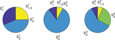
Variance decompositions (classical ANOVA) under $F_{\mathbf{X}}^1$, $F_{\mathbf{X}}^2$, $F_{\mathbf{X}}^3$.

Let us consider now the mixture path. The first step is the assignment of the distribution weights, $\mathrm{\Pi }$. If the analyst poses the three distributions as equally likely, i.e., $\mathrm{\Pi }=\{\frac{1}{3},\frac{1}{3},\frac{1}{3}\}$, by Equation (22), we obtain the mixture distribution $P_{\mathbf{X}}={\sum }_{q=1}^3\frac{1}{3}{F}_{\mathbf{X}}^q$. Numerically, for the mixture sample, we randomly mix the data generated under each distribution to obtain a unique (mixture) sample of size 9,000. In this way, we follow the two‐step procedure illustrated, among others, in Chick (2001). The marginal density of $X_i$ under $P_{\mathbf{X}}$ is reported in the first panel of Fig. 1 as a dotted line. Note that the shape of the mixture marginal density does not belong to any of the assigned family of parametric distributions. Also, under the mixture distribution, the model inputs become dependent, with a correlation coefficient of about 24%—given the symmetric distribution assignment, the pairwise correlations are equal for the three inputs. The corresponding density of the model output is reported as a dotted line in the second panel of Fig. 1.

Because with this assignment, the inputs have different supports, the results concerning the generalized functional ANOVA of $g$ are governed by Theorem A.1 in Appendix A. The mixture effect functions can be computed analytically and their analytical expressions are reported in Appendix C. To obtain them, we follow the approach reported in Appendix B. Let us start with the choice of the basis function. For the Ishigami function, the following is a natural selection:

$$\begin{array}{ccc}& & {\phi }_1^{(1)}=1,{\phi }_2^{(1)}=\sin x_1;{\phi }_1^{(2)}=1,{\phi }_2^{(2)}={\sin }^2{x}_2;\hfill \\ & & {\phi }_1^{(3)}=1,{\phi }_2^{(3)}=x_3^4.\hfill \end{array}$$ (47)

Note that for $X_1$ and $X_2$, we do not choose a polynomial basis, but opt for $\sin (·)$. This choice profits from our knowledge of the analytical expression of $g$ and allows for a compact expression of the numerically obtained effect functions listed in Equation (47). For comparison purposes, we also run experiments fully polynomial basis functions; however, this choice, while yielding a comparable numerical accuracy, leads to much less compact expressions that are not reported for brevity.

Once the basis functions are identified, we employ the input–output sample to fit the D‐MORPH polynomial. Fitting accuracy is evaluated at alternative testing and training sizes. Table I reports the values of $R^2$, RAAE, and RMAE for $n_{\text{train}}=300$, $n_{\text{test}}=2,700$ and $n_{\text{train}}=8,000$, and $n_{\text{test}}=1,000$ to provide a comparison. Given the small estimation errors, it is safe to proceed with the calculation of the generalized functional ANOVA effect functions. Appendix C reports the approximated analytical expressions of $g_z^{P_{\mathbf{X}}}$ at $n_{\text{train}}=8,000$. These expressions can be compared against the analytical expressions of the mixture effect functions ${\stackrel{\sim }{g}}_z$. Fig. 3 offers a graphical comparison. (To compare the second‐order effect function $g_{1,3}(x_1,x_3)$, we plot the truth plot for ${\stackrel{\sim }{g}}_{1,3}(x_1,x_3)$ with respect to $g_{1,3}^{P_{\mathbf{X}}}(x_1,x_3)$).

Table I.

D‐MORPH Performance Measures for the Ishigami Function at $n_{\text{train}}=300$ ($n_{\text{test}}=2,700$) and $n_{\text{train}}=8,000$ ($n_{\text{test}}=1,000$)

Data	$n_{\text{train}}=300$			$n_{\text{train}}=8,000$
	$R^2$	RAAE	RMAE	$R^2$	RAAE	RMAE
Training	1.0000	0.0003	0.0019	1.0000	0.0003	0.0029
Testing	1.0000	0.0003	0.0033	1.0000	0.0003	0.0025

Fig 3.

The comparison of the ANOVA effect functions of $g_z^{P_{\mathbf{X}}}$ constructed from 8,000 points with the effect functions of ${\stackrel{\sim }{g}}_z$.

Fig. 3 shows that in spite of $g_z^{P_{\mathbf{X}}}$ being a continuous function, the mixture effect functions ${\stackrel{\sim }{g}}_z$ are the union of three functions whose expression is valid on three disjoint domains. Some functions have large differences (e.g., ${\stackrel{\sim }{g}}_1$, ${\stackrel{\sim }{g}}_3$), and some do not (e.g., ${\stackrel{\sim }{g}}_2$). Moreover, the three functions ${\stackrel{\sim }{g}}_i$, $i\in \{1,2,3\}$, are not smoothly connected to one another. However, their sum is still exactly equal to $g(\mathbf{x})$ that demonstrates the validity of Theorem A.1. Moreover, the results in Appendix A imply that the generalized ANOVA effect functions $g_z^{P_{\mathbf{X}}}$ satisfy the zero mean and the hierarchical orthogonality conditions, and we have proven that the mixture effect functions ${\stackrel{\sim }{g}}_z$ do not (Proposition A.2). Tables C1 and C2 in Appendix C provide numerical evidence of these facts for the Ishigami example.

Regarding variance decomposition for the mixture path, we have the following results. Let us start with the overall variance decomposition in Equation (33). The estimated simulator output variance is $\widehat{\mathbb{V}}[G]=11.46$ and the mean values under the three distributions are ${\widehat{\mathbb{E}}}_1[G]=3.50$, ${\widehat{\mathbb{E}}}_2[G]=3.02$, and ${\widehat{\mathbb{E}}}_3[G]=5.38$, respectively. This leads to an estimated $\widehat{{\stackrel{\sim }{V}}^c}=1.55$. This value indicates that at about $13\%$ of the simulator output variance is due to variations in the simulator output mean value. To assess the structural and correlative contributions, we compute the SCSA sensitivity indices. Using covariance decomposition from the generalized functional ANOVA expansion, we obtain the values reported in Table II.

Table II.

SCSA and Mixture Sensitivity Indices Computed Using $n_{train}=8,000$

$z$	$S_i^a$	$S_i^b$	$S_i$	$B_i$	$T_i$	$B{T}_i$
1	0.21	0.01	0.22	0.17	0.40	0.29
2	0.53	0.01	0.54	0.62	0.54	0.71
3	0.04	0.01	0.05	0.09	0.23	0.12
First‐order sum	0.77	0.03	0.81
(1, 3)	0.19	−0.01	0.18	0.12
Total sum	0.96	0.035	1.00	0.89

The second and third columns of Table II display the values of the structural $S_z^a$ and the correlative $S_z^b$ contributions to the sensitivity indices. The values indicate a small effect of correlations. Overall, the values of $S_i$ show that $X_2$ is the most important simulator input, with $S_2=0.54$. This input is not involved in interactions and $T_2=S_2$. The second most important input is $X_1$, followed by $X_3$. These two inputs are involved in a significant interaction, with $S_{1,3}=0.18$. Table II also reports, for comparison, the mixture indices in Equation (28) (see Appendix A.2) normalized dividing by $\mathbb{V}[g(\mathbf{X})]$. These values are in column 5 of Table II, while column 7 reports the total mixture indices. The ranking agreement between the SCSA and mixture indices in Table II is reassuring for an analyst wishing to know the most important input. However, the mixture indices do not account for the contribution of the inputs to the overall model output variance (see Equation (25)), because they exclude the portion of the variance associated with the variation in the model output mean. In the present analysis, the fraction of variance unexplained by these indices is estimated at about $87\%$, with the remaining $13\%$ explained by the variation in the mean value across the three distributions. Thus, they do not fully convey the input variance‐based importance under $P_{\mathbf{X}}$, which is instead univocally yielded by the SCSA indices.

6. A REALISTIC APPLICATION: THE DICE SIMULATOR DATA SET

The DICE 2007 model has been the basis of several computer experiments for uncertainty and sensitivity analysis, with the first uncertainty quantification performed in Nordhaus (2008). Starting point of these investigations has been the assignment of distributions for eight relevant model inputs identified after a screening analysis: these distributions are indeed judgmental and have been estimated by the author. Other researchers would make, and other studies have made different assessments of the values of these parameters (Nordhaus, 2008, p. 126). In fact, subsequent works such as Millner, Dietz, and Heal (2013), Hu et al. (2012), Butler, Reed, Fisher‐Vanden, Keller, and Wagener (2014), Anderson, Borgonovo, Galeotti, and Roson (2014) perform uncertainty analysis of the DICE model assigning distributions to the model inputs different from the ones originally assigned by Nordhaus (2008).

The DICE model has undergone several revisions and updates over the years. The data set available here contains realizations drawn from the 2007 version. Specifically, the available data are the input–output runs of the DICE simulator under the 19 distributions taken from the uncertainty analysis performed in (Hu et al., 2012, p. 34, Section 4.3). In Hu et al. (2012), uncertainty in the DICE input distributions is modeled allowing the standard deviations a 50% decrease and a 20% increase. The 19 distributions are as follows: $(1)$ the first distribution is Nordhaus' original distribution; $(2)$ distributions $F_{\mathbf{X}}^q(\mathbf{x})$ $(q=2,\text{…},17)$ are normal with one of the input variances shifted to its lower $(q=2,\text{…},9)$/upper value $(q=10,\text{…},17)$, respectively, with the remaining fixed at the reference values given in Table III; $(3)$ $F_{\mathbf{X}}^{18}(\mathbf{x})$, and $F_{\mathbf{X}}^{19}(\mathbf{x})$ are normal distributions with all model input variances at their lowest and highest values, respectively. We assign $\mathrm{\Pi }=\{p_1,p_2,\text{…},p_{19}\}$, with $p_1=p_{18}=p_{19}=\frac{1}{5}$, and $p_i(i\ne 1,18,19)=\frac{1}{40}$.

Table III.

Distributions Assigned in the Original Uncertainty Analysis of the DICE Model Performed by Nordhaus (2008) and Variations Ranges (Lower and Upper Values) for the Model Input Standard Deviations (${\sigma }_i$). See Nordhaus (2008, p. 127, table 7–1)

$X_i$	Model input name	Mean	${\sigma }_i$	Lower	Upper
$X_1$	Total factor productiv. growth	0.0092	0.004	0.0020	0.0048
$X_2$	Initial sigma growth	0.007	0.002	0.0010	0.0024
$X_3$	Climate sensitivity	3	1.11	0.5550	1.332
$X_4$	Damage function exponent	0.0028	0.0013	0.0006	0.00156
$X_5$	Cost of backstop in 2005	1170	468	234	561.6
$X_6$	POPASYM	8600	1892	946	2270.4
$X_7$	$b_{12}$ in carbon trans. matrix	0.189	0.017	0.0085	0.0204
$X_8$	Cumulative fossil fuel extr.	6,000	1,200	600	1,440

The DICE model produces forecasts for several outputs. As quantity of interest, we consider atmospheric temperature in 2105. We start with the multiple scenario approach. The numerical cost of the analysis is $19,000$ model runs, with samples of $N=1,000$ generated quasi‐Monte Carlo for each distribution. In a multiple scenario approach, the analyst obtains a set of $8\times 19$ global sensitivity indices estimates ${\widehat{S}}_i^q$, $i=1,2,\text{…},8$ and $q=1,2,\text{…},19$. The results must then be analyzed under a robust sensitivity setting (see Section 3.2). In our case, ${\widehat{S}}_3^q>{\widehat{S}}_i^q$ for all $i=1,2,\text{…},8$, $i\ne 3$, and all $q$. That is, $X_3$ is consistently ranked first across all $19$ scenarios, with sensitivity indices varying from a minimum of $S_3^4=0.7$ under $F_{\mathbf{X}}^4(\mathbf{x})$ to a maximum of $S_3^6=0.86$ under $F_{\mathbf{X}}^6(\mathbf{x})$. However, no robust ranking is registered for the second, third, fourth, and fifth most important model inputs, while $X_7$, $X_1$, and $X_8$ robustly rank sixth, seventh, and eight under all distributions.

We then consider the case in which the analyst posits $\mathrm{\Pi }$ and uses a linear mixture. In this case, the distribution is $P_{\mathbf{X}}$ as discussed above and the model output variance is ${\mathbb{V}}^{P_{\mathbf{X}}}[G]=0.3260$. Once $\mathrm{\Pi }$ is assigned, the analyst can use the mixture sensitivity indices. The cost for estimating these indices is the same as that for a multiple scenario approach. In fact, these indices are just an average of the variance‐based contributions obtained under each of the $19$ distributions. Fig. 4 reports the values of ${\stackrel{\sim }{BT}}_i$ and compares them to the corresponding total SCSA indices, whose computation we are to discuss shortly. As one notes, the mixture indices deliver a unique ranking of the inputs. If we compare this ranking to the ranking produced under the multiple scenario approach, we observe that the rankings are generally consistent; for instance, the rankings of $X_3$, $X_7$, $X_1$, and $X_8$ coincide. However, the rankings cannot be completely compared, because the multiple scenario analysis does not provide a unique ranking. Again, the mixture indices provide a quick way to synthesize the multiple scenario information, but they remain exposed to the limitations discussed previously.

Fig 4.

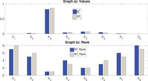
Graph (a): ${\stackrel{\sim }{BT}}_i$ and $S{T}_i$; graph (b) corresponding input ranks.

We finally come to the SCSA indices. For their calculation, a data set of size $5,000$ is obtained by randomly mixing $1,000$ realizations from $F_{\mathbf{X}}^1(\mathbf{x})$,$F_{\mathbf{X}}^{18}(\mathbf{x})$,, and $F_{\mathbf{X}}^{19}(\mathbf{x})$ and 125 realizations for each of $F_{\mathbf{X}}^q(\mathbf{x})(q\ne 1,18,19)$. From Table III, we see that the magnitudes of the model inputs are on different scales, with differences up to ${10}^7$. For numerical stability, we therefore standardize the model input realizations (by subtracting the means and dividing by their standard deviations) before applying the D‐MORPH regression to the mixed data set. As polynomial basis for the DMORPH regression, we use monomials of order lower than or equal to 2 for each input. Sample sizes of 500 are used for training and testing, respectively. To study the accuracy of the results, the regression is replicated 100 times with randomly drawn training and testing sets from the available sample of size 5,000. The results are reported in Table IV.

Table IV.

The Mean and Standard Deviations of the Accuracy and Error Measures $R^2$, RAAE, and RMAE with 100 Replicates

Data	$R^2$		RAAE		RMAE
	mean	std	mean	std	mean	std
Training	0.9996	0.0000	0.0144	0.0007	0.0730	0.0073
Testing	0.9990	0.0002	0.0215	0.0012	0.1988	0.0578

Because the accuracy level is satisfactory, we can trust the D‐MORPH estimates of the generalized functional ANOVA effect functions and global sensitivity indices. We start with the results for the first‐order generalized ANOVA effect functions. Results show that only the first‐order effect functions (see Appendix D for the analytical expressions) are relevant, while the second‐order effect functions are negligible, and not reported. These facts show that the response of the DICE output is mainly additive, with quadratic dependence on all eight model inputs.

Regarding variance decomposition and the calculation of global sensitivity indices, we have the following results. Starting with Proposition A.4, we register ${\stackrel{\sim }{V}}^c=7.10\times {10}^{-4}$. Thus, the contribution coming from the variance of the mean of the model output is negligible. Then, $\mathbb{V}[G]$ is determined mainly by the remaining two components in Equation (33), ${\stackrel{\sim }{V}}^a$ and ${\stackrel{\sim }{V}}^b$. These are estimated, respectively, at ${\stackrel{\sim }{V}}^a=0.3322$ and ${\stackrel{\sim }{V}}^b=-0.0069$. These estimates show an apparent negligible contribution from the correlative part of the variance decomposition. The calculation of the SCSA indices helps us in further understanding this result. Table V reports the values of all eight first‐order and the six most relevant second‐order SCSA indices. To evaluate accuracy, the estimation of the SCSA indices was replicated 100 times with randomly chosen training realizations. Fig. 5 reports the boxplots of the $S_i^a$ and $S{T}_i^a$ indices.

Table V.

First‐ and Second‐Order SCSA Sensitivity Indices for the DICE Model under $P_{\mathbf{X}}$

Rank	$X_j$ or ($X_i,X_j$)	$S_z^a$	$S_z^b$	$S_z$
1	$X_3$	0.8431	−0.0113	0.8317
2	$X_5$	0.0561	−0.0033	0.0528
3	$X_4$	0.0225	0.0057	0.0282
4	$X_6$	0.0341	−0.0191	0.0150
5	$X_7$	0.0066	0.0056	0.0122
6	$X_2$	0.0124	−0.0040	0.0084
7	$X_1$	0.0013	−0.0015	−0.0003
8	$X_8$	0.0001	0.0002	0.0003
First‐order sum		0.9761	−0.0278	0.9483
1	($X_3,X_5$)	0.0136	0.0038	0.0175
2	($X_3,X_4$)	0.0134	0.0018	0.0152
3	($X_4,X_6$)	0.0045	0.0050	0.0095
4	($X_5,X_6$)	0.0040	−0.0004	0.0036
5	($X_4,X_5$)	0.0042	−0.0035	0.0007
6	($X_2,X_5$)	0.0005	−0.0009	−0.0004
Second‐order sum		0.0427	0.0067	0.0493
Total sum		1.0188	−0.0211	0.9976

Fig 5.

The boxplots of $S_i^a$ and the total sensitivity indices $S{T}_i^a$ under $P_{\mathbf{X}}$ obtained from 100 replicates.

The results in Fig. 5 show little variation in the estimates across the replicates, indicating that the values in Table V can be trusted in ranking the inputs. In this respect, most $S_z^b$ are smaller than ${10}^{-2}$, with the exception of $S_3^b$ and $S_6^b$ that have magnitudes 0.0113 and 0.0191, respectively. These values signal that the presence of the mixture causes weak correlations among $X_3$, $X_6$ and the remaining model inputs. Fig. 4 shows that while the ranking between the mixture of indices and the generalized indices is the same for the first and second most important inputs, there are differences in the ranking of the remaining inputs. The fact that the two key drivers of uncertainty are identified by both indices is reassuring, but the coincidence is not guaranteed by an underlying theory. It is also interesting to observe that the disagreement concerns the inputs for which the multiple distribution path does not produce a unique ranking.

Overall, the insights of the multiple scenario path as well as of the SCSA indices show that even if we are uncertain in the model input distributions, $X_3$ stands out as the input on which temperature in 2105 is most sensitive.

7. DISCUSSION

How to represent uncertainty has been a subject of intense investigation in the risk analysis literature, since early works such as Iman and Hora (1990), Iman and Helton (1991), Kaplan and Garrick (1981), Paté‐Cornell (1996), and Apostolakis (1990). These works have spurred a scientific discussion continued in works such as Garrick (2010), Aven (2010), North (2010), Paté‐Cornell (2012), and Flage et al. (2013) in which nonprobabilistic representations of uncertainty are also discussed (see Aven (2020) for a recent critical review). From such works, the literature has discussed several aspects, among which we recall the distinction between aleatory and epistemic uncertainty. Within this context, the probability distribution of the inputs is the first‐level (aleatory) distribution. At the aleatory level, the analyst assigns distributions to the uncertain model inputs (any of these distributions is $F_{\mathbf{X}}^q$). Uncertainty about the aleatory distribution is called epistemic uncertainty (in economics, uncertainty about the true probability distribution is call ambiguity; (Borgonovo & Marinacci, 2015)). The analyst may express epistemic uncertaint yassigning a second‐order distribution. In a global sensitivity analysis context, if the analyst is not sure about the distribution, then she may regard the step of assigning alternative distributions as a preliminary step: the analyst wishes to explore results produced by the model under alternative assumptions concerning the input distribution. This choice is what we called the multiple distribution path. This path is, from a technical viewpoint, closer to the traditional unique distribution analysis. It is, in fact, a repetition of the analysis carried out under a unique distribution as many times as many are the plausible distributions that the analyst wishes to explore. The analyst can derive insights on any of the sensitivity analysis settings under each of the assigned distributions. Should one or more of the model inputs constantly emerge as important in the various assignments, then the analyst may robustly conclude that these inputs are important and represent areas where further modeling/information collection is more worth.

If the analyst assigns a second‐order distribution or has fitted a unique distribution that is the mixture of $Q$ plausible distributions, then she is following a mixture path. Here, we have a number of consequences. Several of them are technical and involve items such as whether the component functions of the functional ANOVA expansion remain orthogonal or whether global sensitivity indices can be reconstructed from the component functions that one obtains under each distribution (see Appendix A for technical details). We point out that even if inputs are independent under each of the assigned distributions, they become dependent once these distributions are linearly mixed. Also, further technical complications emerge if alternative support (ranges) is assigned to the inputs under these alternative distributions.

Then, to obtain variance‐based global sensitivity measures, the analyst needs to use a generalized ANOVA approach, in general. In this case, natural sensitivity measures become the SCSA sensitivity indices that convey information about the structural and the correlative contributions of the inputs. Computationally, the implementation builds on the steps of a traditional uncertainty analysis. It requires the analyst to generate a sample from the mixture distribution (this step would be performed anyway as part of the uncertainty analysis) and then to process such a sample with a numerical technique that allows the estimation of the terms of the generalized functional ANOVA expansion and of the generalized variance‐based sensitivity indices. For this task, the analyst can resort to the D‐MORPH regression, which we have used here.

Overall, the analyst has to consider a number of aspects before performing a global sensitivity analysis when she is uncertain about the input distribution (let us refer to the qualitative decision diagram in Fig. 6).

Fig 6.

Selection path for sensitivity analysis when the analyst is uncertain about the input distribution.

The first item to consider is whether the analyst feels that she is in a position to carry out an uncertainty quantification. We may foresee two main alternatives. In the first, the analyst does not feel that the current state of information allows her/him to assign one or more distributions (downward path in the first node of the tree in Fig. 6). This is typical in a preliminary modeling phase or might be the case for problems in which a distribution cannot be assigned due to lack of data. The analyst can then either opt for running the model over some deterministic scenarios of interest (see, among others [Tietje, 2005] on the creation and definition of scenarios) or may wish not to run the model at all. In that case, we would be in a position in which the whole quantitative risk assessment exercise cannot be carried out or the numbers communicated to the policymaker are not meaningful.

Consider now the upper branch in the qualitative tree of Fig. 6. The analyst may be in a position to assign one or more distributions. If the analyst is satisfied with (can assign) a unique distribution, then, for a variance‐based sensitivity analysis: (i) if the inputs are independent, she can adopt the classical functional ANOVA approach; and (ii) if the inputs are dependent, she needs to adopt a generalized functional ANOVA approach. In the case the analyst is uncertain about the distribution, then she can follow the multiple distribution path. In this case, if independence holds, then the analyst can proceed by performing one classical ANOVA experiment per distribution, otherwise by performing one generalized ANOVA experiment per distribution. Finally, if the analyst adopts a mixture path and recovers a unique distribution, then a generalized ANOVA approach is needed for the computation of global sensitivity indices, in general.

However, there are ways in which an analyst can assign mixture distributions that preserve independence. A first way is to mix only marginal distributions. Suppose that an analyst assigns $Q_i$ marginal distributions to the uncertain input $X_i$ ($Q_i\ge 1$). We denote these distributions with $F_{i,1}(x_i)$, $F_{i,2}(x_i),\text{…}$, $F_{i,Q_i}(x_i)$. Then, if these distributions are mixed marginally, the analyst obtains the marginal distribution of each input as

$$F_i(x_i)=\sum _{s=1}^{Q_i}{\alpha }_{i,s}{f}_{i,s}(x_i)$$ (48)

with weights ${\sum }_{s=1}^m{\alpha }_{i,s}=1$ and ${\alpha }_{i,s}\ge 0$ for all $i=1,2,\text{…},n$ and $s=1,2,\text{…},Q_i$. Then, assigning the product distribution $F_{\mathbf{X}}(x)={\prod }_{i=1}^n{F}_i(x_i)$ leads to the overall distribution

$$\begin{array}{ccc}\hfill F_{\mathbf{X}}(x)& & =\prod _{i=1}^n{F}_i(x_i)=\prod _{i=1}^n\sum _{s=1}^{Q_i}{\alpha }_{i,s}{f}_{i,s}(x_i)\hfill \\ & & =\sum _{t=1}^{Q_1+Q_2+\cdots +Q_n}{q}_t\prod _{i=1}^n{h}_i(x_i)\hfill \end{array}$$ (49)

with the weights $q_s$ and $h_i(x_i)$ defined by appropriate combinations of the ${\alpha }_{i,s}$ and the marginal densities assigned to $X_i$, respectively. The resulting distribution $F_{\mathbf{X}}(x)$ is unique and still a product measure. A second way of combining distributions that maintains independence is the logarithmic opinion pool (see also Borgonovo et al., 2018 for further discussion). In this case, the analyst assigns $Q$ possible product measures to all inputs, that is, $F_{\mathbf{X}}^q(\mathbf{x})={\prod }_{i=1}^n{F}_i^q(x_i)$, and then combines these $Q$ distributions via

$$F_{\mathbf{X}}^{LogPool}(\mathbf{x})=k\prod _{q=1}^Q{\left(F_{\mathbf{X}}^q(\mathbf{x})\right)}^{w_q}=k\prod _{q=1}^Q{\left(\prod _{i=1}^n{F}_i^q(x_i)\right)}^{w_q}$$ (50)

with $w_q$ such that ${\sum }_{q=1}^Q{w}_q=1$ and $w_q\ge 0$. Note that $F_{\mathbf{X}}^{LogPool}(\mathbf{x})$ is still a product measure and thus preserves independence. If either marginal mixing or logpool mixing is a choice that accommodates the risk analyst degree of belief about the inputs, then one obtains a mixture distribution that preserves independence. Then, to obtain variance‐based sensitivity measures, one can resort to the classical ANOVA expansion.

In the multiple choice path, an interesting question is whether we may have some a priori knowledge that there will be no rank reversals when considering the alternative distributions. Experiments carried out by the authors suggest that this might be the case when the assigned distributions and supports do not differ significantly. However, the analysis can be made rigorous only if there is some analytical result for a specific form of the input–output mapping and for specific distributions. Indeed, the following counterexample shows that there cannot be a universal result. Consider the case in which $X_i$ is the most important input when the distribution is $F_{\mathbf{X}}^q$. If, in an alternative scenario, say $q+1$, $X_i$ is assigned a Dirac‐delta measure, then any global sensitivity measure associated with $X_i$ would be equal to zero under $F_{\mathbf{X}}^{q+1}$, causing $X_i$ to join the group of the least important inputs. Such a “$q+1$” scenario would represent when the analyst is certain in the exact value of parameter $X_i$.

Example 7

(Example 2 continued) For the Ishigami model, consider a fourth distributional assignment in which $X_2$ is assigned a Dirac‐delta measure and $X_1$ and $X_3$ are kept uniform in $[-\pi ,\pi ]$. Then $X_2$ would become the least important input under this distributional assignment.

8. CONCLUSIONS

The presence of competing model input distributions creates issues in the global sensitivity analysis of computer codes concerning the theory, the implementation, as well as the interpretation of variance‐based results.

We have seen that (i) an approach looking at results under each alternative distribution may not lead to definitive conclusions due to ranking variability; (ii) when independence does not hold under each distribution, an approach based on the mixture of functional ANOVA expansions loses interpretability; (iii) if the analyst assigns a mixture of the plausible distributions, an approach based on the generalized functional ANOVA expansion allows her to regain uniqueness in the expansion and to estimate global sensitivity indices.

While our work has evidenced and addressed some of the main issues that are open by the simultaneous removal of the independence and unique distribution assumptions, further research is needed. On the one hand, the performance of additional numerical experiments can lead further insights on the proposed approach. It is not excluded that the use of a variance‐based approach simultaneously with other global methods such as distribution‐based methods could lead to additional relevance insights, maintaining the same computational burden. Also, in the present work, we have principally focused on a factor prioritization setting. The exploration of the consequences of removing the unique distribution assumption on other settings, such as trend identification and interaction quantification, is a relevant problem that may result in a further research avenue.

APPENDIX A. DETAILED QUANTITATIVE TREATMENT OF THE CLASSICAL AND GENERALIZED FUNCTIONAL ANOVA EXPANSION

A.1. Generalized Functional ANOVA

The functional ANOVA expansion is a central tool in uncertainty quantification. It provides a formal background for applications ranging from smoothing spline ANOVA models (Lin et al., 2000; Ma & Soriano, 2018), generalized regression models (Kaufman & Sain, 2010; Huang, 1998), and global sensitivity analysis (Durrande et al., 2013). Owen (2013) accurately reviews its historical development, highlighting its origin in Fisher and Mackenzie (1923) and Hoeffding (1948) and the alternative proofs that have been provided over the years (Efron & Stein, 1981; Sobol', 1993; Takemura, 1983). These proofs rely on the assumption that the model inputs are independent. The proof of the existence and uniqueness of a functional ANOVA representation under input dependence is due to Hooker (2007), Li et al. (2010), and Chastaing et al. (2012). Let

$$g:\mathcal{X}\to \mathbb{R},\mathbf{x}=(x_1,\text{…},x_n)\mapsto y=g(\mathbf{x})$$ (A1)

denote the simulator input–output mapping, where $\mathcal{X}\subset {\mathbb{R}}^n$ and $n$ is the number of inputs. Under uncertainty, let $(\mathcal{X},\mathcal{B}(\mathcal{X}),\mathbb{P})$, $\mathbb{P}:\mathcal{B}(\mathcal{X})\to [0,1]$ denote the simulator input probability space. The symbol $F_{\mathbf{X}}(\mathbf{x})=\mathbb{P}\circ {\mathbf{X}}^{-1}(\xi \in \mathcal{X}:\xi \le \mathbf{x})$ denotes the joint input cumulative distribution function (cdf), the symbol $f_{\mathbf{X}}(\mathbf{x})$ denotes the probability density function (pdf). For simplicity in the remainder, we shall also use the abbreviated notation $F=F_{\mathbf{X}}(\mathbf{x})$ to denote the distribution of the model inputs. Uncertainty in $\mathbf{X}$ reverberates in the simulator output, which becomes a function of random variable $G=g(\mathbf{X})$. We assume throughout that $g\in {\mathcal{L}}^2(\mathcal{X})$. Then, let us consider the set $Z=\{1,2,\text{…},n\}$ of the $n$ model input indices, and let $2^Z$ denote the associated power set. Here, $z\in 2^Z$ denotes a generic subset of indices. Hooker (2007) proves that $g(\mathbf{x})$ has a uniquefunctional ANOVA expansion as presented in Equation (6). In Equation (6), the effect functions $g_z^F({\mathbf{x}}_z)$ are determined by the weak annihilating conditions (Li & Rabitz, 2012; Rahman, 2014)

$${\int }_{{\mathcal{X}}_i}{g}_z^F({\mathbf{x}}_z)f_z({\mathbf{x}}_z)d{x}_i=0,\text{for}\text{all}i\in z,$$ (A2)

where $f_z({\mathbf{x}}_z)$ is the marginal density of ${\mathbf{X}}_z$, or equivalently by the hierarchical orthogonality conditions

$$\begin{array}{ccc}& & {\int }_{{\mathcal{X}}_z}{g}_z^F({\mathbf{x}}_z)h({\mathbf{x}}_v)d{F}_z({\mathbf{x}}_z)=0,\text{for}\text{all}h\in {\mathcal{L}}^2({\mathcal{X}}_v),\hfill \\ & & v\subset z,z\ne \varnothing .\hfill \end{array}$$ (A3)

The functions $g_z^F$ are called the effect functions of the generalized functional ANOVA expansion and can be retrieved from the nested equations

(A4)

denotes the subset $Z\setminus z$. To illustrate, for $z=\{i\}$

$$\begin{array}{ccc}\hfill g_i^F(x_i)& & ={\int }_{{\mathcal{X}}_{\sim i}}g(\mathbf{x})d{F}_{\sim i}({\mathbf{x}}_{\sim i})-g_0^F\hfill \\ & & -\sum _{\{i\}\subset v\in 2^Z}{\int }_{{\mathcal{X}}_{\sim i}}{g}_v^F({\mathbf{x}}_v)d{F}_{\sim i}({\mathbf{x}}_{\sim i}).\hfill \end{array}$$ (A5)

Therefore, the determination of the generalized functional ANOVA expansion requires the solution of a system of nested equations. If the model inputs are independent, then the last term in Equation (A4) vanishes, and Equation (A4) reduces to

$$g_z^F({\mathbf{x}}_z)={\int }_{{\mathcal{X}}_{\sim z}}g(\mathbf{x})d{F}_{\sim z}({\mathbf{x}}_{\sim z})-\sum _{v\subset z}{g}_v^F({\mathbf{x}}_v).$$ (A6)

In this case, the effect functions of the expansion given in Equation (6) are no longer nested and can be computed sequentially starting from $g_0^F$ (Li & Rabitz, 2012). For independent inputs, the weak annihilating condition of Equation (A2) becomes the strong annihilating condition of Equation (7) and the hierarchical orthogonality condition of Equation (A3) then reduces to the strong (mutual) orthogonality condition of Equation (8). One calls Equation (6) the generalized functional ANOVA expansion of $g$, if the weak orthogonality conditions in Equation (A3) apply; one calls Equation (6) the classical expansion if the measure $F_{\mathbf{X}}(\mathbf{x})$ is a product measure and the strong orthogonality conditions in Equation (8) apply.

The generalized functional ANOVA expansion leads to a corresponding generalized decomposition of the model output variance, ${\mathbb{V}}^F[G]$ (Li & Rabitz, 2012) presented in Equation (14). One then defines the classical variance‐based sensitivity indices by normalization (Homma & Saltelli, 1996; Sobol', 1993):

$$S_z^F=V_z^F/{\mathbb{V}}^F[G].$$ (A7)

The sensitivity index in Equation (A7) is called the variance‐based sensitivity index of group $z$ for all $z\in 2^Z$, $z\ne \varnothing$, and represents the contribution to $\mathbb{V}[G]$ of the residual interaction of variables with indices in $z$. For independent inputs, all covariances and consequently all $S_z^{b,F}$ are zero, and the indices $S_z^F$ in Equation (15) coincide with the classical variance‐based sensitivity indices in Equation (A7).

A.2. Functional ANOVA with Multiple Distributions

We first investigate the properties of the functional ANOVA effect functions, starting with the two‐path coincidence mentioned in Section 2.2. For generality, we also remove the assumption that the supports of the distributions are the same and consider $F_{\mathbf{X}}^q$, $q=1,2,\text{…},Q$, with corresponding measure spaces $({\mathcal{X}}_q,\mathcal{B}({\mathcal{X}}_q),F_{\mathbf{X}}^q)$, with ${\mathcal{X}}_q\subseteq \mathcal{X}$ for all $q=1,2,\text{…},Q$. This situation can arise in an expert elicitation if two or more experts provide different opinions about the ranges in which a given quantity may lay. We may have ${\mathcal{X}}_1\cap {\mathcal{X}}_2\cap \cdots \cap {\mathcal{X}}_Q=\varnothing$, as well as all other possible intersections, and the union of the supports may not exhaust the domain $\mathcal{X}$, ${\bigcup }_{q=1}^Q{\mathcal{X}}_q\subset \mathcal{X}$. Of course, the analyst may decide to restrict the support to ${\bigcup }_{q=1}^Q{\mathcal{X}}_q$, so that the overall $\mathcal{X}$ is indeed the union of the supports provided by the experts. However, in the following mathematical treatment, this assumption is not essential.

The next results concern the question of whether, when we relax the independence and unique distribution assumptions, we can still obtain the same representation in Equation (23), given that we follow the two paths discussed before (all proofs are in Appendix A.3).

Theorem A.1

Suppose that the analyst has posed $\mathcal{F}=\{F_{\mathbf{X}}^1,F_{\mathbf{X}}^2,\text{…},F_{\mathbf{X}}^Q\}$ with supports ${\mathcal{X}}_1,{\mathcal{X}}_2,\text{…},{\mathcal{X}}_Q$ and a prior $\mathrm{\Pi }=(p_1,\text{…},p_Q)$ on $\mathcal{F}$. Let $g(\mathbf{x})$ be square integrable under any $F_{\mathbf{X}}^q\in \mathcal{F}$. Denote the joint support of $\mathbf{x}\in \mathcal{X}$ with $Q(\mathbf{x})=\{q:\mathbf{x}\in {\mathcal{X}}_q\}$. Then,

$$g(\mathbf{x})=\sum _{z\in 2^Z}{\stackrel{\sim }{g}}_z({\mathbf{x}}_z),$$ (A8)

where

$${\stackrel{\sim }{g}}_z({\mathbf{x}}_z)=\sum _{q\in Q(\mathbf{x})}{\displaystyle \frac{p_q}{{\sum }_{j\in Q(\mathbf{x})}{p}_{q_j}}}{g}_z^q({\mathbf{x}}_z).$$ (A9)

In the case where the distributions have identical supports, the following holds.

Corollary A.1

If ${\mathcal{X}}_1={\mathcal{X}}_2=\cdots ={\mathcal{X}}_Q$, then at any point $\mathbf{x}\in \mathcal{X}$, it holds

$${\stackrel{\sim }{g}}_z({\mathbf{x}}_z)=\sum _{q=1}^Q{p}_q{g}_z^q({\mathbf{x}}_z).$$ (A10)

For the second path, we have the following.

Proposition A.1

Let $P_{\mathbf{X}}={\sum }_{q=1}^Q{p}_q{F}_{\mathbf{X}}^q$. Then:

$$g=\sum _{z\in 2^Z}{\stackrel{\sim }{\stackrel{\sim }{g}}}_z,$$ (A11)

where

$${\stackrel{\sim }{\stackrel{\sim }{g}}}_z=\sum _{p=1}^Q{p}_q{g}_z^{P_{\mathbf{X}},q}({\mathbf{x}}_z),$$ (A12)

where $g_z^{P_{\mathbf{X}},q}({\mathbf{x}}_z)$ are given as integrals of the effect function $g_z^{P_{\mathbf{X}}}$ under $P_{\mathbf{X}}$.

The functions ${\stackrel{\sim }{\stackrel{\sim }{g}}}_z$ in Proposition A.1 are different from the functions ${\stackrel{\sim }{g}}_z$ in Theorem A.1. Thus, the coincidence of the two paths discussed in Section 2.2 is not valid under general distributional assumptions. More in detail, the coincidence under independence is possible because we can proceed in the functional ANOVA decomposition by induction. For nonproduct measures $\mathcal{F}$, however, the generalized functional ANOVA expansion terms contains the higher order effect functions

$$\sum _{v\cap z\ne \varnothing ,v\not\subset z}{\int }_{{\mathcal{X}}_{\sim z}}{g}_v^{P_{\mathbf{X}}}({\mathbf{x}}_v)d{P}_{\sim z}({\mathbf{x}}_{\sim z}),$$

and induction cannot be applied.

Concerning orthogonality, we have the following result.

Proposition A.2

Let ${\mathcal{X}}_1={\mathcal{X}}_2=\cdots ={\mathcal{X}}_q=\mathcal{X}$, and let $P_{\mathbf{X}}={\sum }_{q=1}^Q{p}_q{F}_{\mathbf{X}}^q$ be a mixture measure and

$$g(\mathbf{x})=\sum _{z\in 2^Z}{g}_z^q({\mathbf{x}}_z)$$ (A13)

be a generalized functional ANOVA expansion of $g$ with respect to $F_{\mathbf{X}}^q$. Then, a mixture of generalized functional ANOVA expansions of $g$ with respect to each measure $F_{\mathbf{X}}^q$

$$\begin{array}{ccc}\hfill g(\mathbf{x})& & =\sum _{q=1}^Q{p}_q\left(\sum _{z\in 2^Z}{g}_z^q({\mathbf{x}}_z)\right)=\sum _{z\in 2^Z}\left(\sum _{q=1}^Q{p}_q{g}_z^q({\mathbf{x}}_z)\right)\hfill \\ & & =\sum _{z\in 2^Z}{\stackrel{\sim }{g}}_z({\mathbf{x}}_z)\hfill \end{array}$$

does not satisfy the hierarchical orthogonality conditions and is generally not a generalized functional ANOVA expansion of $g$ with respect to every possible mixture measure $P_{\mathbf{X}}$ consistent with $g$.

To address the consequences on monotonicity formally, let us recall that a multivariate mapping $g:\mathcal{X}\to \mathbb{R}$ is nonincreasing (nondecreasing) if $g(\mathbf{x}+\mathbf{t})\le (\ge )g(\mathbf{x})$ for all $\mathbf{x},\mathbf{x}+\mathbf{t}\in \mathcal{X}$, $\mathbf{t}\ge \mathbf{0}$.

Proposition A.3

Let ${\mathcal{X}}_1={\mathcal{X}}_2=\cdots ={\mathcal{X}}_q=\mathcal{X}$. If $g$ is nondecreasing, $P_{\mathbf{X}}={\sum }_{q=1}^Q{p}_q{F}_{\mathbf{X}}^q$ and

$$g(\mathbf{x})=\sum _{z\in 2^Z}{g}_z^{P_{\mathbf{X}}}({\mathbf{x}}_z)$$ (A14)

is the generalized functional ANOVA expansion of $g$ with respect to $P_{\mathbf{X}}$, the first‐order effect functions $g_i^{P_{\mathbf{X}}}(i=1,2,\text{…},n)$ may not retain the monotonicity of $g$.

For $g_i^{P_{\mathbf{X}}}(x_i)$ to respect the monotonicity of $g$ with respect to $x_i$, one needs to add conditions on the behavior of the last term ${\sum }_{v\cap z\ne \varnothing ,v\not\subset z}{\int }_{{\mathcal{X}}_{\sim z}}{g}_v^{P_{\mathbf{X}}}({\mathbf{x}}_v)d{P}_{\sim z}({\mathbf{x}}_{\sim z})$ in Equation (A4).

We have the following consequences on variance decomposition.

Proposition A.4

Let ${\mathbb{V}}^{P_{\mathbf{X}}}[G]$ denote the variance of the simulator output. Under the mixture $P_{\mathbf{X}}={\sum }_{q=1}^Q{p}_q{F}_{\mathbf{X}}^q$, we have

$$\begin{array}{ccc}\hfill {\mathbb{V}}^{P_{\mathbf{X}}}[G]& =& \sum _{q=1}^Q{p}_q\left(\sum _{\varnothing \ne z\in 2^Z}\left[V_z^q+\mathrm{Cov}\left(g_z^q({\mathbf{X}}_z),\sum _{z\ne v\in 2^Z}{g}_v^q({\mathbf{X}}_v)\right)\right]\right.\hfill \\ & & \left.+{({\mathbb{E}}_q[G]-\mathbb{E}[G])}^2\right),\hfill \end{array}$$ (A15)

so that

$${\mathbb{V}}^{P_{\mathbf{X}}}[G]={\stackrel{\sim }{V}}^a+{\stackrel{\sim }{V}}^b+{\stackrel{\sim }{V}}^c,$$ (A16)

where

$$\begin{array}{ccc}\hfill {\stackrel{\sim }{V}}^a& =& \sum _{q=1}^Q{p}_q\sum _{\varnothing \ne z\in 2^Z}{V}_z^q=\sum _{\varnothing \ne z\in 2^Z}{\stackrel{\sim }{B}}_z,\hfill \end{array}$$ (A17)

$$\begin{array}{ccc}\hfill {\stackrel{\sim }{V}}^b& =& \sum _{q=1}^Q{p}_q\sum _{\varnothing \ne z\in 2^Z}\mathrm{Cov}\left({\displaystyle g_z^q({\mathbf{X}}_z),\sum _{z\ne v\in 2^Z}{g}_v^q({\mathbf{X}}_v)}\right),\hfill \end{array}$$ (A18)

$$\begin{array}{ccc}\hfill {\stackrel{\sim }{V}}^c& =& {\displaystyle \sum _{q=1}^Q{p}_q{({\mathbb{E}}_q[G]-\mathbb{E}[G])}^2={\mathbb{V}}_{\mathrm{\Pi }}\{\mathbb{E}(G)\}.}\hfill \end{array}$$ (A19)

The equality in Equation (A15) results in a generalization of Equation (25), and thus of Equation (1), with the appearance of correlative terms in the variance decomposition. That is, the variance of the model output in the case of mixtures of nonproduct distributions is equal to the contribution provided by the mixture of structural variance contributions, ${\stackrel{\sim }{V}}^a$, the mixture of the correlative contributions, ${\stackrel{\sim }{V}}^b$, and the residual fraction related to the variation of the expected value of $Y$ over the distributions in $\mathcal{F}$, ${\stackrel{\sim }{V}}^c$. Note that the fractions differ from the mixture of the normalized structural and correlative sensitivity indices, as

$${\displaystyle \frac{{\stackrel{\sim }{V}}^a}{{\mathbb{V}}^{P_{\mathbf{X}}}[G]}}\ne \sum _{q=1}^Q{p}_q{\displaystyle \frac{{\stackrel{\sim }{V}}^{a,q}}{{\mathbb{V}}^q[G]}},\mathrm{and}{\displaystyle \frac{{\stackrel{\sim }{V}}^b}{{\mathbb{V}}^{P_{\mathbf{X}}}[G]}}\ne \sum _{q=1}^Q{p}_q{\displaystyle \frac{{\stackrel{\sim }{V}}^{b,q}}{{\mathbb{V}}^q[G]}}.$$ (A20)

A.3. Proofs

Proof of Theorem A.1

First, on the entire $\mathcal{X}$ and for $q=1,2,\text{…},Q$, let us define the functions

$$g^q(\mathbf{x})=\left\{\begin{array}{cc}{\displaystyle {\sum }_{z\in 2^Z}{g}_z^q,}\hfill & \text{if}\mathbf{x}\in {\mathcal{X}}_q,\hfill \\ g(\mathbf{x}),\hfill & \text{otherwise},\hfill \end{array}\right.$$

and

$$h(\mathbf{x})=\sum _{q=1}^Q{p}_q{g}^q(\mathbf{x}).$$

Then, we show that $h(\mathbf{x})=g(\mathbf{x})$. We have the following cases. Case A): ${\mathcal{X}}_1\cap {\mathcal{X}}_2\cap \cdots \cap {\mathcal{X}}_Q=\varnothing$; in this case, the supports of the distributions are disjoint. Note that it is not necessarily true that ${\bigcup }_{q=1}^Q{\mathcal{X}}_q=\mathcal{X}$. Consider a point $\mathbf{x}\in \mathcal{X}$. Then, it is either $\mathbf{x}\in {\mathcal{X}}_q$ for some $q$, or $\mathbf{x}\in \mathcal{X}\setminus {\cup }_{q=1}^Q{\mathcal{X}}_q$. If $\mathbf{x}\in {\mathcal{X}}_q$, then

$$\begin{array}{ccc}\hfill h(\mathbf{x})& & =\sum _{q=1}^Q{p}_q{g}^q(\mathbf{x})=p_q\sum _{z\in 2^Z}{g}_z^q(\mathbf{x})\hfill \\ & & +g(\mathbf{x})\sum _{s=1,s\ne q}^Q{p}_s=p_{q}g(\mathbf{x})+g(\mathbf{x})(1-p_q)=g(\mathbf{x}).\hfill \end{array}$$

Conversely, if $\mathbf{x}\in \mathcal{X}\setminus {\cup }_{q=1}^Q{\mathcal{X}}_q$, then $h(\mathbf{x})={\sum }_{q=1}^Q{p}_{q}g(\mathbf{x})=g(\mathbf{x}){\sum }_{q=1}^Q{p}_q=g(\mathbf{x})$. Thus, in Case A) $h(\mathbf{x})=g(\mathbf{x})$ for all points $\mathbf{x}\in \mathcal{X}$. Case B), there are some nonnull intersections among some (or all) of the supports. In particular, consider $\mathbf{x}$ belonging to a support ${\mathcal{X}}_q={\mathcal{X}}_{q_1}\cap {\mathcal{X}}_{q_2}\cdots \cap {\mathcal{X}}_{q_k}\ne \varnothing$. Then, at $\mathbf{x}$, we have

$$\begin{array}{ccc}\hfill h(\mathbf{x})& & =\sum _{q=1}^Q{p}_q{g}^q(\mathbf{x})=\sum _{q\in \{q_1,q_2,\text{…},q_k\}}{p}_q{g}^q(\mathbf{x})\hfill \\ & & +g(\mathbf{x})\sum _{q\notin \{q_1,q_2,\text{…},q_k\}}{p}_q.\hfill \end{array}$$ (A21)

Then, because for each generalized functional ANOVA expansion, we have $g^q(\mathbf{x})=g(\mathbf{x})$, and this equality becomes

$$\begin{array}{ccc}\hfill h(\mathbf{x})& =& g(\mathbf{x})\left(\sum _{q\in \{q_1,q_2,\text{…},q_k\}}{p}_q\right)+g(\mathbf{x})\left(\sum _{q\notin \{q_1,q_2,\text{…},q_k\}}{p}_q\right)\hfill \\ & =& g(\mathbf{x})\left(\sum _{q\in \{q_1,q_2,\text{…},q_k\}}{p}_q+\sum _{q\notin \{q_1,q_2,\text{…},q_k\}}{p}_q\right)\hfill \\ & =& g(\mathbf{x}),\hfill \end{array}$$ (A22)

because, by construction, ${\sum }_{q\in \{q_1,q_2,\text{…},q_k\}}{p}_q+{\sum }_{q\notin \{q_1,q_2,\text{…},q_k\}}{p}_q=1$. Then, note that at any other point $\mathbf{x}\in \mathcal{X}$, the point is either belonging to a support that intersects with other supports (Case B) or that does not intersect (Case A); thus, $h(\mathbf{x})=g(\mathbf{x})$.

Then, suppose $\mathbf{x}\in {\mathcal{X}}_q$, for some value of $q\in \{q_1,q_2,\text{…},q_k\}$ and that ${\mathcal{X}}_{q_1}\cap {\mathcal{X}}_{q_2}\cap \cdots \cap {\mathcal{X}}_{q_k}\ne \varnothing$. Then, by item 1, we have $h(\mathbf{x})=g(\mathbf{x})$ at all $\mathbf{x}$, and by Equation (A22), we have:

$$\sum _{q\in \{q_1,q_2,\text{…},q_k\}}{p}_q{g}^q(\mathbf{x})+g(\mathbf{x})\left(\sum _{q\notin \{q_1,q_2,\text{…},q_k\}}{p}_q\right)=g(\mathbf{x}).$$

Then, rearranging, we can write

$$\begin{array}{ccc}\hfill \sum _{q\in \{q_1,q_2,\text{…},q_k\}}{p}_q{g}^q(\mathbf{x})& =& g(\mathbf{x})-g(\mathbf{x})\left(\sum _{q\notin \{q_1,q_2,\text{…},q_k\}}{p}_q\right)\hfill \\ & =& g(\mathbf{x})\left(1-\sum _{q\notin \{q_1,q_2,\text{…},q_k\}}{p}_q\right)\hfill \\ & =& g(\mathbf{x})\left(\sum _{q\in \{q_1,q_2,\text{…},q_k\}}{p}_q\right),\hfill \end{array}$$ (A23)

which leads to

$$\begin{array}{ccc}\hfill g(\mathbf{x})={\displaystyle \frac{{\sum }_{q\in \{q_1,q_2,\text{…},q_k\}}{p}_q{g}^q(\mathbf{x})}{{\sum }_{q\in \{q_1,q_2,\text{…},q_k\}}{p}_q}}& =& {\displaystyle \frac{{\sum }_{q\in \{q_1,q_2,\text{…},q_k\}}{p}_q{\sum }_{z\in 2^Z}{g}_z^q({\mathbf{x}}_z)}{{\sum }_{q\in \{q_1,q_2,\text{…},q_k\}}{p}_q}}\hfill \\ & =& {\displaystyle \frac{{\sum }_{z\in 2^Z}{\sum }_{q\in \{q_1,q_2,\text{…},q_k\}}{p}_q{g}_z^q({\mathbf{x}}_z)}{{\sum }_{q\in \{q_1,q_2,\text{…},q_k\}}{p}_q}},\hfill \end{array}$$

whence

$$g(\mathbf{x})=\sum _{z\in 2^Z}\sum _{q\in \{q_1,q_2,\text{…},q_k\}}{\displaystyle \frac{p_q}{{\sum }_{q\in \{q_1,q_2,\text{…},q_k\}}{p}_q}}{g}_z^q({\mathbf{x}}_z)=\sum _{z\in 2^Z}\stackrel{\sim }{g}{}_z({\mathbf{x}}_z),$$

where

$$\stackrel{\sim }{g}{}_z({\mathbf{x}}_z)=\sum _{q\in \{q_1,q_2,\text{…},q_k\}}{\displaystyle \frac{p_q}{{\sum }_{q\in \{q_1,q_2,\text{…},q_k\}}{p}_q}}{g}_z^q({\mathbf{x}}_z)$$

is the reweighted mixture in Equation (A9).$\square$

Proof of Corollary A.1

If ${\mathcal{X}}_1={\mathcal{X}}_2=\cdots ={\mathcal{X}}_Q$, then ${\mathcal{X}}_{q_1}\cap {\mathcal{X}}_{q_2}\cap \cdots \cap {\mathcal{X}}_{q_k}={\mathcal{X}}_q$ for all $q=1,2,\text{…},Q$ so that in Equation (A9), we have $k=Q$ and ${\sum }_{q\in \{1,2,\text{…},Q\}}{p}_q=1$, so that

$$\stackrel{\sim }{g}{}_z({\mathbf{x}}_z)=\sum _{q=1}^Q{p}_q{g}_z^q({\mathbf{x}}_z).$$

$\square$

Proof of Proposition A.1

First, the supports of the $Q$ distributions need not to be the same. For simplicity, suppose that under the $F_{\mathbf{X}}^q$, $\mathbf{X}$ is a continuous random vector. We can write

$$\begin{array}{ccc}\hfill P_z& =& \int \cdots \int \sum _{q=1}^Q{p}_q{f}_{\mathbf{X}}^q(\mathbf{x})d{\mathbf{x}}_{\sim z}\hfill \\ & =& \sum _{q=1}^Q{p}_q\int \cdots \int f_{\mathbf{X}}^{q}d{\mathbf{x}}_{\sim z}=\sum _{q=1}^Q{p}_q{F}_z^q,\hfill \end{array}$$

and similarly, $P_{\sim z}={\sum }_{q=1}^Q{p}_q{F}_{\sim z}^q$, from which d$P_{\sim z}={\sum }_{q=1}^Q{p}_q$d$F_{\sim z}^q$. Then, let us consider the first component of the generalized functional ANOVA decomposition of a three‐variate mapping:

$$\begin{array}{ccc}\hfill g_i^{P_{\mathbf{X}}}(x_i)& =& {\int }_{{\mathcal{X}}_{\sim i}}g(\mathbf{x})d{P}_{\sim i}({\mathbf{x}}_{\sim i})-g_0^{P_{\mathbf{X}}}\hfill \\ & -& {\int }_{{\mathcal{X}}_j}{g}_{i,j}^{P_{\mathbf{X}}}(x_i,x_j)d{P}_j(\mathbf{x})\hfill \end{array}$$ (A24)

$$\begin{array}{ccc}& -& {\int }_{{\mathcal{X}}_k}{g}_{i,k}^{P_{\mathbf{X}}}(x_i,x_k)d{P}_k(\mathbf{x})\hfill \\ & -& {\int }_{{\mathcal{X}}_{j,k}}{g}_{i,j,k}^{P_{\mathbf{X}}}(x_i,x_j,x_k)d{P}_{j,k}(\mathbf{x})\hfill \end{array}$$ (A25)

where $g_{i,j}^{P_{\mathbf{X}}}(x_i,x_j)$, $g_{i,k}^{P_{\mathbf{X}}}(x_i,x_k)$ and $g_{i,j,k}^{P_{\mathbf{X}}}(x_i,x_j,x_k)$ are the effect functions of the generalized functional ANOVA expansion of $g(\mathbf{x})$ under $P_{\mathbf{X}}(\mathbf{x})$. For clarity, it is useful to introduce the functions

$$h_i^{P_{\mathbf{X}}}(x_i)={\int }_{{\mathcal{X}}_{\sim i}}g(\mathbf{x})d{P}_{\sim i}({\mathbf{x}}_{\sim i}),$$ (A26)

$$h_{i|j}^{P_{\mathbf{X}}}(x_i)={\int }_{{\mathcal{X}}_j}{g}_{i,j}^{P_{\mathbf{X}}}(x_i,x_j)d{P}_j(x_j)$$ (A27)

and

$$h_{i|j,k}^{P_{\mathbf{X}}}(x_i)={\int }_{{\mathcal{X}}_{j,k}}{g}_{i,j,k}^{P_{\mathbf{X}}}(x_i,x_j,x_k)d{P}_{j,k}(\mathbf{x}).$$ (A28)

We can then rewrite the previous equation as:

$$g_i^{P_{\mathbf{X}}}(x_i)=h_i^{P_{\mathbf{X}}}(x_i)-h_{i|j}^{P_{\mathbf{X}}}(x_i)-h_{i|k}^{P_{\mathbf{X}}}(x_i)-h_{i|j,k}^{P_{\mathbf{X}}}(x_i)-g_0^{P_{\mathbf{X}}}.$$ (A29)

Because at $\mathbf{x}$, $P_{\mathbf{X}}(\mathbf{x})={\sum }_{q=1}^Q{p}_q{F}_{\mathbf{X}}^q(\mathbf{x})$, one can write

$$\begin{array}{ccc}\hfill h_i^{P_{\mathbf{X}}}(x_i)& =& {\int }_{{\mathcal{X}}_{\sim i}}g(\mathbf{x})\sum _{q=1}^Q{p}_{q}d{F}_{\sim i}^q=\sum _{q=1}^Q{p}_q{\int }_{{\mathcal{X}}_{\sim i}^q}g(\mathbf{x})d{F}_{\sim i}^q\hfill \\ & =& \sum _{q=1}^Q{p}_q{h}_i^q(x_i).\hfill \end{array}$$ (A30)

Similarly, for $h_{i|j}^{P_{\mathbf{X}}}(x_i)$ one finds:

$$\begin{array}{ccc}\hfill h_{i|j}^{P_{\mathbf{X}}}(x_i)& =& \sum _{q=1}^Q{p}_q{\int }_{{\mathcal{X}}_j^q}{g}_{i,j}^{P_{\mathbf{X}}}(x_i,x_j)d{F}_j^q\hfill \\ & =& \sum _{q=1}^Q{p}_q{h}_{i|j}^{P,q}(x_i),\hfill \end{array}$$ (A31)

where $h_{i|j}^{P,q}(x_i)={\int }_{{\mathcal{X}}_j^q}{g}_{i,j}^{P_{\mathbf{X}}}(x_i,x_j)d{F}_j^q$. A similar expression holds for $h_{i|k}^{P_{\mathbf{X}}}(x_i)$. For $h_{i|j,k}^{P_{\mathbf{X}}}(x_i)$, one has

$$\begin{array}{ccc}\hfill h_{i|j,k}^{P_{\mathbf{X}}}(x_i)& =& {\int }_{{\mathcal{X}}_{j,k}}{g}_{i,j,k}^{P_{\mathbf{X}}}(x_i,x_j,x_k)d{P}_{j,k}(\mathbf{x})\hfill \\ & =& {\int }_{{\mathcal{X}}_{j,k}}{g}_{i,j,k}^{P_{\mathbf{X}}}(x_i,x_j,x_k)\sum _{q=1}^Q{p}_{q}d{F}_{j,k}^q(x_j,x_k)\hfill \\ & =& \sum _{q=1}^Q{p}_q{\int }_{{\mathcal{X}}_{j,k}^q}{g}_{i,j,k}^{P_{\mathbf{X}}}(x_i,x_j,x_k)d{F}_{j,k}^q(\mathbf{x})\hfill \\ & =& \sum _{q=1}^Q{p}_q{h}_{i|j,k}^{P,q}(x_i),\hfill \end{array}$$ (A32)

where $h_{i|j,k}^{P,q}(x_i)={\int }_{{\mathcal{X}}_{j,k}^q}{g}_{i,j,k}^{P_{\mathbf{X}}}(x_i,x_j,x_k)d{F}_{j,k}^q(x_j,x_k)$. Finally, for $g_0$ one has:

$$g_0=\sum _{q=1}^Q{p}_q{g}_0^q,$$ (A33)

with

$$g_0^q={\int }_{\mathcal{X}}g(\mathbf{x})d{F}_{\mathbf{X}}^q(\mathbf{x}).$$ (A34)

In summary, one obtains:

$$\begin{array}{ccc}\hfill g_i^{P_{\mathbf{X}}}(x_i)& =& \sum _{q=1}^Q{p}_q\left[h_i^q(x_i)-g_0^q-h_{i|k}^{P,q}(x_i)-h_{i|j}^{P,q}(x_i)\right.\hfill \\ & & \left.-h_{i|j,k}^{P,q}(x_i)\right].\hfill \end{array}$$ (A35)

Then, letting $g_i^{P_{\mathbf{X}},q}(x_i)=h_i^q(x_i)-g_0^q-h_{i|j}^{P_{\mathbf{X}},q}(x_i)-h_{i|k}^{P_{\mathbf{X}},q}(x_i)-h_{i|j,k}^{P_{\mathbf{X}},q}(x_i)$, one can write

$$g_i^{P_{\mathbf{X}}}(x_i)=\sum _{q=1}^Q{p}_q{g}_i^{P_{\mathbf{X}},q}(x_i).$$ (A36)

The procedure can be repeated for any subset of indices $z$. Then,

$$g=\sum _{z\in 2^Z}\sum _{p=1}^Q{p}_q{g}_z^{P_{\mathbf{X}},q}(x_z),$$ (A37)

and letting ${\stackrel{\sim }{\stackrel{\sim }{g}}}_z={\sum }_{p=1}^Q{p}_q{g}_z^{P_{\mathbf{X}},q}(x_z)$, one has

$$g=\sum _{z\in 2^Z}{\stackrel{\sim }{\stackrel{\sim }{g}}}_z.$$ (A38)

$\square$

Proof of Proposition A.2

For the proof, we only need to prove that each ${\stackrel{\sim }{g}}_z({\mathbf{x}}_z)$ may not satisfy the weak annihilating condition for every possible mixture measure $P_{\mathbf{X}}$ consistent with $g$. The weak annihilating condition requires that

$$\begin{array}{ccc}\hfill \int {\stackrel{\sim }{g}}_z({\mathbf{x}}_z)p_{{\mathbf{x}}_z}({\mathbf{x}}_z)d{x}_{i_r}& =& \int \sum _{q=1}^Q{p}_q{g}_z^q({\mathbf{x}}_z)p_{{\mathbf{x}}_z}({\mathbf{x}}_z)d{x}_{i_r}\hfill \\ & =& 0,i_r\in z\hfill \end{array}$$ (A39)

where $|z|$ is the cardinality of $z=\{i_1,i_2,\text{…},i_{|z|}\}$, and $p_{{\mathbf{x}}_z}({\mathbf{x}}_z)$ is the marginal pdf of $P_{\mathbf{X}}$ for ${\mathbf{x}}_z$.

$$\begin{array}{ccc}\hfill \int {\stackrel{\sim }{g}}_z({\mathbf{x}}_z)p_{{\mathbf{x}}_z}({\mathbf{x}}_z)d{x}_{i_r}& =& \sum _{q=1}^Q{p}_q\int g_z^q({\mathbf{x}}_z)p_{{\mathbf{x}}_z}({\mathbf{x}}_z)d{x}_{i_r}\hfill \\ & =& \sum _{q=1}^Q{p}_q\int g_z^q({\mathbf{x}}_z)\sum _{q^{\prime }=1}^Q{p}_{q^{\prime }}{f}_{{\mathbf{x}}_z}^{q^{\prime }}({\mathbf{x}}_z)d{x}_{i_r}\hfill \\ & =& \sum _{q=1}^Q{p}_q\left(\sum _{q^{\prime }=1}^Q{p}_{q^{\prime }}\int g_z^q({\mathbf{x}}_z)f_{{\mathbf{x}}_z}^{q^{\prime }}({\mathbf{x}}_z)d{x}_{i_r}\right),\hfill \end{array}$$ (A40)

where $f_{{\mathbf{x}}_z}^{q^{\prime }}({\mathbf{x}}_z)$ is the marginal pdf of $F_{\mathbf{X}}^{q^{\prime }}$ for ${\mathbf{x}}_z$. Since $g_z^q({\mathbf{x}}_z)$ is an effect function of the generalized functional ANOVA expansion of $g$ with respect to $F_{\mathbf{X}}^q$, the weak annihilating condition

$$\int g_z^q({\mathbf{x}}_z)f_{{\mathbf{x}}_z}^q({\mathbf{x}}_z)d{x}_{i_r}=0$$ (A41)

holds. Substituting Equation (A41) into Equation (A40) yields

$$\begin{array}{c}\hfill \int {\stackrel{\sim }{g}}_z({\mathbf{x}}_z)p_{{\mathbf{x}}_z}({\mathbf{x}}_z)d{x}_{i_r}=\sum _{q=1}^Q{p}_q\left(\sum _{q^{\prime }=1,q^{\prime }\ne q}^Q{p}_{q^{\prime }}\int g_z^q({\mathbf{x}}_z)f_{{\mathbf{x}}_z}^{q^{\prime }}({\mathbf{x}}_z)d{x}_{i_r}\right).\end{array}$$ (A42)

Due to Equation (A41), there must exist measures $F_{\mathbf{X}}^{q^{\prime }}$ different from $F_{\mathbf{X}}^q$ such that

$$\int g_z^q({\mathbf{x}}_z)f_{{\mathbf{x}}_z}^{q^{\prime }}({\mathbf{x}}_z)d{x}_{i_r}\ne 0.$$ (A43)

If this were not true, i.e.,

$$\int g_z^q({\mathbf{x}}_z)f_{{\mathbf{x}}_z}^{q^{\prime }}({\mathbf{x}}_z)d{x}_{i_r}=0$$ (A44)

holds for all possible (it can be infinite) measures $F_{\mathbf{X}}^{q^{\prime }}$ consistent with $g$, then

$$g_z^q({\mathbf{x}}_z)\equiv 0.$$ (A45)

This is true for any subset $z$. If all $g_z^q({\mathbf{x}}_z)\equiv 0$, then $g(\mathbf{x})$ is a constant, which contradicts to that $g(\mathbf{x})$ is an arbitrary square integrable function. Therefore, the weak annihilating condition may not hold for ${\stackrel{\sim }{g}}_z^q({\mathbf{x}}_z)$, and

$$g(\mathbf{x})=\sum _{z\in 2^Z}{\stackrel{\sim }{g}}_z({\mathbf{x}}_z)$$

may not be a generalized functional ANOVA expansion.$\square$

Proof of Proposition A.3

When the simulator inputs distribution is a mixture of the model input distributions, the resulting distribution $P_{\mathbf{X}}$ is not a product measure, no matter whether each of the $F_{\mathbf{X}}^q$'s is a product measure or not. Therefore, Equation (A14) is a generalized functional ANOVA expansion. The generic first order effect function is given by

$$\begin{array}{ccc}\hfill g_i^{P_{\mathbf{X}}}(x_i)& =& {\int }_{{\mathcal{X}}_{\sim i}}g(\mathbf{x})d{P}_{{\mathbf{x}}_{\sim i}}({\mathbf{x}}_{\sim i})-f_0\hfill \\ & -& \sum _{\{i\}\subset v\subseteq 2^Z}{\int }_{{\mathcal{X}}_{\sim i}}{g}_v^{P_{\mathbf{X}}}({\mathbf{x}}_v)d{P}_{{\mathbf{x}}_{\sim i}}({\mathbf{x}}_{\sim i}).\hfill \end{array}$$

Even if the first term on the right hand side is non‐decreasing, the subtraction of the ${\sum }_{\{i\}\subset v\in 2^Z}{\int }_{{\mathcal{X}}_{\sim i}}{g}_v^{P_{\mathbf{X}}}({\mathbf{x}}_v)d{P}_{{\mathbf{x}}_{\sim i}}({\mathbf{x}}_{\sim i})$ term does not guarantee that

$$g_i^{P_{\mathbf{X}}}(x_i)\le g_i^{P_{\mathbf{X}}}(x_i+h_i),\text{for}\text{all}{h}_i>0.$$ (A46)

Hence, the first order effect functions $g_i^{P_{\mathbf{X}}}(i=1,2,\text{…},n)$ may not retain the monotonicity of $g$.$\square$

Proof of Proposition A.4

By the law of total variance we have:

$$\begin{array}{ccc}\hfill {\mathbb{V}}^{P_{\mathbf{X}}}[G]& =& {\mathbb{E}}_{\mathrm{\Pi }}\{{\mathbb{V}}_q[G]\}+{\mathbb{V}}_{\mathrm{\Pi }}\{\mathbb{E}[G]\}\hfill \end{array}$$ (A47)

$$\begin{array}{ccc}& =& \sum _{q=1}^Q{p}_q{\mathbb{V}}_q[G]+{\mathbb{V}}_{\mathrm{\Pi }}\{\mathbb{E}[G]\}\hfill \end{array}$$ (A48)

where the inner variances and expectations are taken with $\mathbf{X}$ being distributed according to $F_{\mathbb{X}}^q\in \mathcal{F}$. If the measures in $\mathcal{F}$ are generic then by Equations (14) and (A48) we can write

$$\begin{array}{ccc}\hfill {\mathbb{V}}^{P_{\mathbf{X}}}[G]& =& \sum _{q=1}^Q{p}_q\left[{\mathbb{V}}_z^q+\mathrm{Cov}\left(g_z^q({\mathbf{X}}_z),\sum _{z\ne v\in 2^Z}{g}_v^q({\mathbf{X}}_v)\right)\right]\hfill \\ & +& {\mathbb{V}}_{\mathrm{\Pi }}\{\mathbb{E}[G]\}.\hfill \end{array}$$ (A49)

Then, rewriting the above equation, one obtains

$$\begin{array}{ccc}\hfill {\mathbb{V}}^{P_{\mathbf{X}}}[G]& =& \sum _{q=1}^Q{p}_q{\mathbb{V}}_z^q+\sum _{q=1}^Q{p}_q\mathrm{Cov}\left(g_z^q({\mathbf{X}}_z),\sum _{z\ne v\in 2^Z}{g}_v^q({\mathbf{X}}_v)\right)\hfill \\ & +& {\mathbb{V}}_{\mathrm{\Pi }}\{\mathbb{E}[G]\}.\hfill \end{array}$$ (A50)

Notice that

$${\mathbb{V}}_{\mathrm{\Pi }}\{\mathbb{E}[G]\}=\sum _{q=1}^Q{p}_q{({\mathbb{E}}_q[G]-\mathbb{E}[G])}^2,$$ (A51)

so, it is also a weighted average over the measures in $\mathcal{F}$. One therefore obtains

$${\mathbb{V}}^{P_{\mathbf{X}}}[G]={\stackrel{\sim }{V}}^a+{\stackrel{\sim }{V}}^b+{\stackrel{\sim }{V}}^c.$$ (A52)

$\square$

APPENDIX B. DETAILS ON THE D‐MORPH REGRESSION

A sufficient condition for respecting hierarchical orthogonality of the effect functions of a generalized functional ANOVA expansion is that the basis functions of any lower order effect function span a subspace normal to the subspace spanned by the basis functions of the nested higher order effect functions. Specifically, consider that $V$ is a Hilbert subspace spanned by $\{v_1,v_2,\text{…},v_k\}$, and a larger subspace $U(\supset V)$ is spanned by $\{v_1,v_2,\text{…},v_k,v_{k+1},\text{…},v_m\}$, $m>k$. Then, we have the decomposition $U=V\oplus V^{\perp }$, where $V^{\perp }$ and $V$ are orthogonal. Note that there always exists a vector in $V^{\perp }$ (i.e., a linear combination of $v_1,v_2,\text{…},v_k,v_{k+1},\text{…},v_m$) orthogonal to all vectors in $V$. Then, let $g\in {\mathcal{L}}^2(\mathcal{X},\mathcal{B}(\mathcal{X}),F)$. Note that if the basis functions of a first order effect function are a subset of the basis functions in the nested second order ones the generalized ANOVA effect functions meet the hierarchical orthogonality conditions. Using the approximation scheme in Equation (42), one obtains the second order generalized functional ANOVA expansion for $g(\mathbf{x})$ as

$$\begin{array}{ccc}\hfill g(\mathbf{x})& \approx & g_0^F+\sum _{i=1}^n\sum _{r=1}^k{\alpha }_r^{(0)i}{\phi }_r^{(i)}(x_i)+\sum _{1\le i<j\le n}\left[\sum _{r=1}^k{\alpha }_r^{(ij)i}{\phi }_r^{(i)}(x_i)\right.\hfill \\ & & +\left.\sum _{r=1}^k{\alpha }_r^{(ij)j}{\phi }_r^{(j)}(x_j)+\sum _{p=1}^l\sum _{q=1}^l{\beta }_{pq}^{(0)ij}{\phi }_p^{(i)}(x_i){\phi }_q^{(j)}(x_j)\right].\hfill \end{array}$$ (B1)

The unknown parameters $\{\alpha \}$, $\{\beta \}$ can be obtained through a least‐squares regression from an input‐output sample $({\mathbf{x}}^{(s)},g({\mathbf{x}}^{(s)}))$, $s=1,2,\text{…},N$, in which the input realizations follow the distribution $F$. Equation (B1) can be written in vector form as

$$\mathit{\varphi }{({\mathbf{x}}^{(s)})}^T\mathbf{c}=g({\mathbf{x}}^{(s)})-g_0^F,(s=1,2,\text{…},N)$$ (B2)

where $\mathbf{c}$ is a $t$‐dimensional vector composed of all the unknown parameters $\{\alpha \}$, $\{\beta \}$. In matrix form we can write Equation (B2) as $\mathbf{\Phi }\mathbf{c}=\mathbf{b}$, and by least‐squares we obtain

$${\mathbf{\Phi }}^T\mathbf{\Phi }\mathbf{c}={\mathbf{\Phi }}^T\mathbf{b}.$$ (B3)

Because the basis functions of the first order effect functions are also used in the second order effect functions, some equations in (B3) are duplicate and can be removed to obtain a rectangular algebraic equation system $A\mathbf{c}=\mathbf{d}$. Such a system is consistent and has an infinite number of solutions for $\mathbf{c}$ with the general form

$$\mathbf{c}=A^{+}\mathbf{d}+(\mathrm{I}-A^{+}A)\mathbf{u},$$ (B4)

where $\mathbf{u}$ is an arbitrary vector, $\mathrm{I}$ is an identity matrix and $A^{+}$ is the generalized inverse of $A$ satisfying all four Penrose conditions (Rao & Mitra, 1971). The infinite number of solutions for $\mathbf{c}$ produced by the arbitrary vector $\mathbf{u}$ compose a convex set $\mathcal{M}$ which provides a possibility to search for a specific solution satisfying an extra requirement along an exploration path $\mathbf{c}(s)$ with a single parameter $s\in [0,\infty )$ within $\mathcal{M}$. This search process can be characterized by a differential equation obtained by differentiating both sides of Equation (B4) with respect to $s$

$$\frac{d\mathbf{c}(s)}{ds}=(\mathrm{I}-A^{+}A)\frac{d\mathbf{u}(\mathbf{s})}{ds}=P\mathbf{v}(s)$$ (B5)

where $P=(\mathrm{I}-A^{+}A)$ is an orthogonal projector satisfying $P=P^2=P^{T}P$. The function vector $\mathbf{v}(s)$ may be chosen so that a specified cost function $\mathcal{K}(\mathbf{c}(s))$ (e.g., model variance, fitting smoothness, or particularly here the hierarchical orthogonality of the ANOVA effect functions) is minimized along the exploration path. Setting

$$\mathbf{v}(s)=-\frac{\partial \mathcal{K}(\mathbf{c}(s))}{\partial \mathbf{c}},$$ (B6)

yields (Li & Rabitz, 2012)

$$\begin{array}{ccc}\hfill \frac{\mathrm{d}\mathcal{K}(\mathbf{c}(s))}{\mathrm{d}s}& =& {\left(\frac{\partial \mathcal{K}(\mathbf{c}(s))}{\partial \mathbf{c}}\right)}^T\frac{\mathrm{d}\mathbf{c}(s)}{\mathrm{d}s}={\left(\frac{\partial \mathcal{K}(\mathbf{c}(s))}{\partial \mathbf{c}}\right)}^{T}P\mathbf{v}(s)\hfill \\ & =& -{\left(P\frac{\partial \mathcal{K}(\mathbf{c}(s))}{\partial \mathbf{c}}\right)}^T\left(P\frac{\partial \mathcal{K}(\mathbf{c}(s))}{\partial \mathbf{c}}\right)\le 0,\hfill \end{array}$$ (B7)

i.e., the $\mathcal{K}$ is continuously lowered as $s\mapsto \infty$ systematically refining the generalized functional ANOVA expansion. Therefore,

$${\mathbf{c}}_{\infty }=\underset{s\to \infty }{\lim }\mathbf{c}(s)$$ (B8)

not only is a solution of the system $A\mathbf{c}=\mathbf{d}$, but also minimizes $\mathcal{K}$ (Li & Rabitz, 2012). If the cost function is a quadratic form in $\mathbf{c}$, $\mathcal{K}=\frac{1}{2}{\mathbf{c}}^{T}B\mathbf{c}$, where $B$ is symmetric and non‐negative definite, ${\mathbf{c}}_{\infty }$ can be found analytically as (Li & Rabitz, 2012):

$${\mathbf{c}}_{\infty }=V_{t-r}{\left(U_{t-r}^T{V}_{t-r}\right)}^{-1}{U}_{t-r}^T{A}^{+}\mathbf{d},$$ (B9)

where $U_{t-r}$, and $V_{t-r}$ are the last $t-r$ columns of matrices $U$ and $V$ obtained from the singular value decomposition of matrix $PB$, where

$$PB=U\left[\begin{array}{cc}{S}_r\hfill & 0\hfill \\ 0\hfill & 0\hfill \end{array}\right]V^T$$ (B10)

with $S_r$ being a diagonal matrix composed of the $r$ non‐zero singular values of $PB$. Equation (B9) is the key formula implementation of the D‐MORPH regression. The solution ${\mathbf{c}}_{\infty }$ is a special linear combination of the elements of $\mathbf{c}=A^{+}\mathbf{d}$ obtained by the least‐squares regression. Note that to determine ${\mathbf{c}}_{\infty }$ one only needs to determine $A^{+}$ and perform the singular value decomposition of matrix $PB$. Finally, we observe that the construction of matrix $B$ defining the hierarchical orthogonality condition of different order ANOVA effect functions is straightforward, but the formulas take a large space. We refer to Li and Rabitz (2012) for the detailed formulation. To evaluate fit, the analyst can use one or more of the following performance measures:

• 1.
  The coefficient of model determination,

  $$R^2=1-\frac{\frac{1}{N}{\sum }_{s=1}^N{(g({\mathbf{x}}^{(s)})-\widehat{g}({\mathbf{x}}^{(s)}))}^2}{{\sigma }^2(g(\mathbf{x}))},$$ (B11)

  where $\widehat{g}({\mathbf{x}}^{(s)})$ is the D‐MORPH prediction value of $g({\mathbf{x}}^{(s)})$ and

  $${\sigma }^2(g(\mathbf{x}))\approx \frac{1}{N}\sum _{s=1}^N{(g({\mathbf{x}}^{(s)})-\overline{g}(\mathbf{x}))}^2,$$ (B12)

  with $\overline{g}(\mathbf{x})$ being the mean value of $g(\mathbf{x})$ for the training or testing data;
• 2.
  The relative average absolute error (RAAE),

  $$\mathrm{RAAE}=\frac{\frac{1}{N}{\sum }_{s=1}^N|g({\mathbf{x}}^{(s)})-\widehat{g}({\mathbf{x}}^{(s)})|}{\sigma (g(\mathbf{x}))},$$ (B13)
• 3.
  The relative maximum absolute error (RMAE),

  $$\mathrm{RMAE}=\frac{{\max }_s|g({\mathbf{x}}^{(s)})-\widehat{g}({\mathbf{x}}^{(s)})|}{\sigma (g(\mathbf{x}))}.$$ (B14)

Accurate fit is registered when $R^2\simeq 1$ and the values of the remaining performance measures close to zero.

APPENDIX C. DETAILED CALCULATIONS FOR THE ISHIGAMI TEST FUNCTION

Given the input‐output mapping of the Ishigami function and the distributions/supports assigned in Section 4.2, one obtains the following analytical expressions of the functional ANOVA expansion also reported in Borgonovo et al. (2018):

• 1.
  Under $F_{\mathbf{X}}^1$ on ${\mathcal{X}}_1={[-\pi ,\pi ]}^3$:

  $$\begin{array}{ccc}\hfill g_0^{F^1}& =& {\displaystyle \frac{a}{2}};\hfill \\ \hfill g_1^{F^1}& =& \sin (x_1)\left(1+b{\displaystyle \frac{{\pi }^4}{5}}\right);\hfill \\ \hfill g_2^{F^1}& =& a{\sin }^2(x_2)-{\displaystyle \frac{a}{2}};\hfill \\ \hfill g_{1,3}^{F^1}& =& b\sin (x_1)\left(x_3^4-{\displaystyle \frac{{\pi }^4}{5}}\right);\hfill \end{array}$$ (C1)
• 2.
  Under $F_{\mathbf{X}}^2$ on ${\mathcal{X}}_2={(-\infty ,\infty )}^3$:

  $$\begin{array}{ccc}\hfill g_0^{F^2}& =& {\displaystyle \frac{a}{2}}(1-e^{-2});\hfill \\ \hfill g_1^{F^2}& =& \sin (x_1)(1+3b);\hfill \\ \hfill g_2^{F^2}& =& a{\sin }^2(x_2)-{\displaystyle \frac{a}{2}}(1-e^{-2});\hfill \\ \hfill g_{1,3}^{F^2}& =& b\sin (x_1)\left(x_3^4-3\right).\hfill \end{array}$$ (C2)
• 3.Under $F_{\mathbf{X}}^3$ on ${\mathcal{X}}_3={[0,\pi ]}^3$:

$$\begin{array}{ccc}\hfill g_0^{F^3}& =& {\displaystyle \frac{a}{2}}+{\displaystyle \frac{2}{\pi }}\left(1+b{\displaystyle \frac{{\pi }^4}{5}}\right);\hfill \\ \hfill g_1^{F^3}& =& \left(\sin (x_1)-{\displaystyle \frac{2}{\pi }}\right)\left(1+b{\displaystyle \frac{{\pi }^4}{5}}\right);\hfill \\ \hfill g_2^{F^3}& =& a{\sin }^2(x_2)-{\displaystyle \frac{a}{2}};\hfill \\ \hfill g_3^{F^3}& =& {\displaystyle \frac{2b}{\pi }}\left(x_3^4-{\displaystyle \frac{{\pi }^4}{5}}\right);\hfill \\ \hfill g_{1,3}^{F^3}& =& b\left(\sin (x_1)-{\displaystyle \frac{2}{\pi }}\right)\left(x_3^4-{\displaystyle \frac{{\pi }^4}{5}}\right).\hfill \end{array}$$ (C3)

Then, with ${\mathrm{\Pi }}_F=\{\frac{1}{3},\frac{1}{3},\frac{1}{3}\}$, by Equation (A9) in Theorem A.1 a mixture ANOVA representation of $g$ on ${\mathbb{R}}^3$ is given by:

• 1.
  If $\mathbf{x}\in {\mathcal{X}}_2\setminus {\mathcal{X}}_1$ with the single distribution $F_{\mathbf{X}}^2$:

  $$\begin{array}{ccc}\hfill {\stackrel{\sim }{g}}_0& =& {\displaystyle \frac{a}{2}}(1-e^{-2});\hfill \\ \hfill {\stackrel{\sim }{g}}_1(x_1)& =& \sin (x_1)(1+3b);\hfill \\ \hfill {\stackrel{\sim }{g}}_2(x_2)& =& a{\sin }^2(x_2)-{\displaystyle \frac{a}{2}}(1-e^{-2});\hfill \\ \hfill {\stackrel{\sim }{g}}_{1,3}(x_1,x_3)& =& b\sin (x_1)\left(x_3^4-3\right).\hfill \end{array}$$ (C4)
• 2.
  If $\mathbf{x}\in {\mathcal{X}}_1\setminus {\mathcal{X}}_3$ with the two distributions $F_{\mathbf{X}}^1,F_{\mathbf{X}}^2$:

  $$\begin{array}{ccc}\hfill {\stackrel{\sim }{g}}_0& =& a\left({\displaystyle \frac{1}{2}}-{\displaystyle \frac{e^{-2}}{4}}\right);\hfill \\ \hfill {\stackrel{\sim }{g}}_1(x_1)& =& \sin x_1\left({\displaystyle \frac{3}{2}}b+{\displaystyle \frac{1}{10}}{\pi }^{4}b+1\right);\hfill \\ \hfill {\stackrel{\sim }{g}}_2(x_2)& =& a\left({\sin }^2{x}_2-{\displaystyle \frac{1}{2}}+{\displaystyle \frac{e^{-2}}{4}}\right);\hfill \\ \hfill {\stackrel{\sim }{g}}_{1,3}(x_1,x_3)& =& {\displaystyle \frac{b\sin x_1}{10}}\left(10x_3^4-{\pi }^4-15\right);\hfill \end{array}$$
• 3.
  If $\mathbf{x}\in {\mathcal{X}}_3$ with all the three distributions:

  $$\begin{array}{ccc}\hfill {\stackrel{\sim }{g}}_0& =& {\displaystyle \frac{1}{2}}a+{\displaystyle \frac{2}{15}}{\pi }^{3}b-{\displaystyle \frac{a{e}^{-2}}{6}}+{\displaystyle \frac{2}{3\pi }};\hfill \\ \hfill {\stackrel{\sim }{g}}_1(x_1)& =& \sin x_1\left(1+b-{\displaystyle \frac{2b}{15}}{\pi }^4\right)\hfill \\ & & -{\displaystyle \frac{2}{3\pi }}-{\displaystyle \frac{2b}{15}}{\pi }^3;\hfill \\ \hfill {\stackrel{\sim }{g}}_2(x_2)& =& a\left({\sin }^2{x}_2-{\displaystyle \frac{1}{2}}+{\displaystyle \frac{e^{-2}}{6}}\right);\hfill \\ \hfill {\stackrel{\sim }{g}}_3(x_1)& =& {\displaystyle \frac{2b}{3\pi }}\left(x_3^4-{\displaystyle \frac{{\pi }^4}{5}}\right);\hfill \\ \hfill {\stackrel{\sim }{g}}_{1,3}(x_1,x_3)& =& {\displaystyle \frac{2}{15}}{\pi }^{3}b-b\sin x_1+b{x}_3^4\sin x_1\hfill \\ & & -{\displaystyle \frac{2}{3\pi }}b{x}_3^4-{\displaystyle \frac{2}{15}}{\pi }^{4}b\sin x_1.\hfill \end{array}$$

The generalized functional ANOVA effect functions at $n_{\text{train}}=8000$ points have the expressions:

$$\begin{array}{ccc}\hfill g_0^{P_{\mathbf{X}}}& =& 3.9550,\hfill \\ \hfill g_1^{P_{\mathbf{X}}}(x_1)& =& 2.3180\sin (x_1)-0.4776,\hfill \\ \hfill g_2^{P_{\mathbf{X}}}(x_2)& =& 7{\sin }^2(x_2)-3.3241,\hfill \\ \hfill g_3^{P_{\mathbf{X}}}(x_3)& =& 0.0277x_3^4-0.3868,\hfill \\ \hfill g_{1,3}^{P_{\mathbf{X}}}(x_1,x_3)& =& 0.1x_3^4\sin (x_1)-0.0277x_3^4\hfill \\ & & -1.3182\sin x_1+0.2335.\hfill \end{array}$$ (C5)

For comparison, with the assigned parameterization of the Ishigami model used in these numerical experiments, the mixture ANOVA effects ${\stackrel{\sim }{g}}_z$ are:

• 1.
  If $\mathbf{x}\in {\mathcal{X}}_2\setminus {\mathcal{X}}_1$ with the single distribution $F_{\mathbf{X}}^2$:

  $$\begin{array}{ccc}\hfill {\stackrel{\sim }{g}}_0& =& 3.0263,\hfill \\ \hfill {\stackrel{\sim }{g}}_1(x_1)& =& 1.3\sin x_1,\hfill \\ \hfill {\stackrel{\sim }{g}}_2(x_2)& =& 7{\sin }^2{x}_2-3.0263,\hfill \\ \hfill {\stackrel{\sim }{g}}_3(x_3)& =& 0,\hfill \\ \hfill {\stackrel{\sim }{g}}_{1,3}(x_1,x_3)& =& 0.1\sin x_1{x}_3^4-0.3\sin x_1.\hfill \end{array}$$ (C6)
• 2.
  If $\mathbf{x}\in {\mathcal{X}}_1\setminus {\mathcal{X}}_3$ with the two distributions $F_{\mathbf{X}}^1,F_{\mathbf{X}}^2$:

  $$\begin{array}{ccc}\hfill {\stackrel{\sim }{g}}_0& =& 3.2632,\hfill \\ \hfill {\stackrel{\sim }{g}}_1(x_1)& =& 2.1241\sin x_1,\hfill \\ \hfill {\stackrel{\sim }{g}}_2(x_2)& =& 7{\sin }^2{x}_2-3.2632,\hfill \\ \hfill {\stackrel{\sim }{g}}_3(x_3)& =& 0,\hfill \\ \hfill {\stackrel{\sim }{g}}_{1,3}(x_1,x_3)& =& 0.1\sin x_1{x}_3^4-1.1241\sin x_1.\hfill \end{array}$$ (C7)
• 3.
  If $\mathbf{x}\in {\mathcal{X}}_3$ with all the three distributions:

  $$\begin{array}{ccc}\hfill {\stackrel{\sim }{g}}_0& =& 3.9677,\hfill \\ \hfill {\stackrel{\sim }{g}}_1(x_1)& =& 2.3988\sin x_1-0.6256,\hfill \\ \hfill {\stackrel{\sim }{g}}_2(x_2)& =& 7{\sin }^2{x}_2-3.3421,\hfill \\ \hfill {\stackrel{\sim }{g}}_3(x_3)& =& 0.0212x_3^4-0.4134,\hfill \\ \hfill {\stackrel{\sim }{g}}_{1,3}(x_1,x_3)& =& 0.1\sin x_1{x}_3^4-1.3988\sin x_1\hfill \\ & & -0.0212x_3^4+0.4134.\hfill \end{array}$$ (C8)

Note that the sum of three ANOVA expansions at any $\mathbf{x}\in \mathcal{X}$ is exactly equal to $g(\mathbf{x})$, which demonstrates the theoretical validity of Theorem A.1. Fig. 3 in main text allows a visual comparison.

Tables C1 and C2 report results of numerical tests concerning the “zero mean” and orthogonality properties of the generalized ANOVA and mixture effect functions. They show that all effect functions obtained under the generalized functional ANOVA decomposition of Equation (C5) satisfy the zero mean (bold face numbers in Table C1) and hierarchical orthogonality conditions (bold face numbers in Table C2), while the corresponding mixture effect functions do not.

Table C1.

The Mean Values of the Effect Functions

	$g_1$	$g_2$	$g_3$	$g_{13}$
$g_z^{p_{\mathbf{X}}}$ (300 points)	0.0000	0.0000	0.0006	−0.0005
$g_z^{p_{\mathbf{X}}}$ (8,000 points)	−0.0002	0.0000	0.0005	−0.0005
${\stackrel{\sim }{g}}_z$ (300 point)	0.2637	0.3351	−0.0073	0.1076
${\stackrel{\sim }{g}}_z$ (8,000 point)	0.2497	0.0288	−0.0107	0.1321

Table C2.

The Inner Product of Effect Functions

	$g_z^{p_{\mathbf{X}}}$		${\stackrel{\sim }{g}}_z$
	300 points	8,000 points	300 points	8,000 points
$⟨g_1,g_2⟩$	−0.0094	0.0613	−0.0119	0.0314
$⟨g_1,g_3⟩$	0.0699	0.0879	0.0045	−0.0047
$⟨g_1,g_{13}⟩$	−0.0001	−0.0002	0.1001	0.1785
$⟨g_2,g_3⟩$	0.0533	0.0462	0.0049	−0.0002
$⟨g_2,g_{13}⟩$	−0.1029	0.0086	−0.0634	0.0536
$⟨g_3,g_{13}⟩$	−0.0004	−0.0006	0.2561	0.2422

APPENDIX D. ADDITIONAL DETAILS ON THE DICE TEST CASE

The first‐order generalized ANOVA effect functions for the DICE model, when the reference distribution is $P_{\mathbf{X}}$, are approximated by the following second‐order polynomials:

$$\begin{array}{ccc}\hfill g_1^{P_{\mathbf{X}}}(x_1)& \approx & -0.0019+0.0199x_1+0.0019x_1^2,\hfill \\ \hfill g_2^{P_{\mathbf{X}}}(x_2)& \approx & -0.0069+0.0628x_2+0.0070x_2^2,\hfill \\ \hfill g_3^{P_{\mathbf{X}}}(x_3)& \approx & 0.0945+0.4706x_3-0.0947x_3^2,\hfill \\ \hfill g_4^{P_{\mathbf{X}}}(x_4)& \approx & -0.0296-0.0645x_4+0.0296x_4^2,\hfill \\ \hfill g_5^{P_{\mathbf{X}}}(x_5)& \approx & 0.0706+0.0790x_5-0.0708x_5^2,\hfill \\ \hfill g_6^{P_{\mathbf{X}}}(x_6)& \approx & 0.0095+0.1029x_6-0.0095x_6^2,\hfill \\ \hfill g_7^{P_{\mathbf{X}}}(x_7)& \approx & -0.0023-0.0451x_7+0.0023x_7^2,\hfill \\ \hfill g_8^{P_{\mathbf{X}}}(x_8)& \approx & 0.0023-0.0059x_8-0.0023x_8^2.\hfill \end{array}$$

REFERENCES

- Anderson, B. , Borgonovo, E. , Galeotti, M. , & Roson, R. (2014). Uncertainty in climate change modelling: Can global sensitivity analysis be of help? Risk Analysis, 34(2), 271–293. [DOI] [PubMed] [Google Scholar]
- Apostolakis, G. E. (1990). The concept of probability in safety assessments of technological systems. Science, 250(4986), 1359–1364. [DOI] [PubMed] [Google Scholar]
- Apostolakis, G. E. (2004). How useful is quantitative risk assessment? Risk Analysis, 24(3), 515–520. [DOI] [PubMed] [Google Scholar]
- Aven, T. (2010). On the need for restricting the probabilistic analysis in risk assessments to variability. Risk Analysis, 30(3), 354–360. ISSN 1539‐6924. [DOI] [PubMed] [Google Scholar]
- Aven, T. (2016). Risk assessment and risk management: Review of recent advances on their foundation. European Journal of Operational Research, 116(2), 235–248. [Google Scholar]
- Aven, T. (2020) Three influential risk foundation papers from the 80s and 90s: Are they still state‐of‐the‐art? Reliability Engineering & System Safety, 193, 106680. [Google Scholar]
- Borgonovo, E. (2006). Measuring uncertainty importance: Investigation and comparison of alternative approaches. Risk Analysis, 26(5), 1349–1361. [DOI] [PubMed] [Google Scholar]
- Borgonovo, E. , & Marinacci, M. (2015). Decision analysis under ambiguity. European Journal of Operational Research, 244(3), 823–836. [Google Scholar]
- Borgonovo, E. , Morris, M. D. , & Plischke, E. (2018). Functional anova with multiple distributions: Implications for the sensitivity analysis of computer experiments. SIAM/ASA Journal on Uncertainty Quantification, 6(1), 397–427. [Google Scholar]
- Butler, M. P. , Reed, P. M. , Fisher‐Vanden, K. , Keller, K. , & Wagener, T. (2014). Identifying parametric controls and dependencies in integrated assessment models using global sensitivity analysis. Environmental Modelling & Software, 59, 10–29. [Google Scholar]
- Chastaing, G. , Gamboa, F. , & Prieur, C. (2012). Generalized Hoeffding‐Sobol decomposition for dependent variables: Application to sensitivity analysis. Electronic Journal of Statistics, 6, 2420–2448. [Google Scholar]
- Chastaing, G. , Gamboa, F. , & Prieur, C. (2015). Generalized Sobol sensitivity indices for dependent variables: Numerical methods. Journal of Statistical Computation and Simulation, 85(7), 1306–1333. [Google Scholar]
- Chick, S. E. (2001). Input distribution selection for simulation experiments: Accounting for input uncertainty. Operations Research, 49(5), 744–758. [Google Scholar]
- Cooke, R. M. (2013). Validating expert judgment. Transactions of the American Nuclear Society, 109, 2192–2195. [Google Scholar]
- Cox, D. C. , & Baybutt, P. (1981). Methods for uncertainty analysis: A comparative survey. Risk Analysis, 1(4), 251–258. [Google Scholar]
- Durrande, N. , Ginsbourger, D. , Roustant, O. , & Carraro, L. (2013). ANOVA kernels and RKHS of zero mean functions for model‐based sensitivity analysis. Journal of Multivariate Analysis, 115, 57–67. [Google Scholar]
- Efron, B. , & Stein, C. (1981). The Jackknife estimate of variance. The Annals of Statistics, 9(3), 586–596. [Google Scholar]
- Fisher, R. A. , & Mackenzie, W. A. (1923). The manurial response of different potato varieties. Journal of Agricultural Science, XIII, 311–320. [Google Scholar]
- Flage, R. , Baraldi, P. , Zio, E. , & Aven, T. (2013). Probability and possibility‐based representations of uncertainty in fault tree analysis. Risk Analysis, 33(1), 121–133. [DOI] [PubMed] [Google Scholar]
- Frey, H. C. (2002). Introduction to special section on sensitivity analysis and summary of NCSU/USDA workshop on sensitivity analysis. Risk Analysis, 22(3), 539–545. [DOI] [PubMed] [Google Scholar]
- Gao, L. , Bryan, B. A. , Nolan, M. , Connor, J. D. , Song, X. , & Zhao, G. (2016). Robust global sensitivity analysis under deep uncertainty via scenario analysis. Environmental Modelling & Software, 76, 154–166. [Google Scholar]
- Garrick, B. J. (2010). Interval analysis versus probabilistic analysis. Risk Analysis, 30(3), 369–370. [DOI] [PubMed] [Google Scholar]
- Glotter, M. J. , Pierrehumbert, R. T. , Elliott, J. W. , Matteson, N. J. , & Moyer, E. J. (2014). A simple carbon cycle representation for economic and policy analyses. Climatic Change, 126(3–4), 319–335. [Google Scholar]
- Helton, J. , & Davis, F. J. (2002). Illustration of sampling‐based methods for uncertainty and sensitivity analysis. Risk Analysis, 22(3), 591–622. [DOI] [PubMed] [Google Scholar]
- Helton, J. C. , & Johnson, J. D. (2011). Quantification of margins and uncertainties: Alternative representations of epistemic uncertainty. Reliability Engineering & System Safety, 96, 1034–1052. [Google Scholar]
- Helton, J. C. , & Sallaberry, C. J. (2009). Computational implementation of sampling‐based approaches to the calculation of expected dose in performance assessments for the proposed high‐level radioactive waste repository at Yucca Mountain, Nevada. Reliability Engineering & System Safety, 94(3), 699–721. ISSN 0951‐8320. 10.1016/j.ress.2008.06.018. [DOI] [Google Scholar]
- Helton, J. C. , Johnson, J. D. , Shiver, A. W. , & Sprung, J. L. (1995). Uncertainty and sensitivity analysis of early exposure results with the MACCS reactor accident consequence model. Reliability Engineering & System Safety, 48(2), 91–127. [Google Scholar]
- Hoeffding, W. (1948). A class of statistics with asymptotically normal distribution. Annals of Mathematical Statistics, 19, 293–325. [Google Scholar]
- Homma, T. , & Saltelli, A. (1996). Importance measures in global sensitivity analysis of nonlinear models. Reliability Engineering & System Safety, 52(1), 1–17. ISSN 0951‐8320. [Google Scholar]
- Hooker, G. (2007). Generalized functional ANOVA diagnostics for high dimensional functions of dependent variables. Journal of Computational and Graphical Statistics, 16(3), 709–732. [Google Scholar]
- Hu, Z. , Cao, J. , & Hong, L. J. (2012). Robust simulation of global warming policies using the DICE model. Management Science, 58(12), 2190–2206. [Google Scholar]
- Huang, J. Z. (1998). Projection estimation in multiple regression with application to functional Anova models. The Annals of Statistics, 26(1), 242–272. [Google Scholar]
- Iman, R. L. (1987). A matrix‐based approach to uncertainty and sensitivity analysis for fault trees. Risk Analysis, 7(1), 21–33. [Google Scholar]
- Iman, R. L. , & Helton, J. C. (1988). An investigation of uncertainty and sensitivity analysis techniques for computer models. Risk Analysis, 8(1), 71–90. [Google Scholar]
- Iman, R. L. , & Helton, J. C. (1991). The repeatability of uncertainty and sensitivity analyses for complex probabilistic risk assessments. Risk Analysis, 11(4), 591–606. [Google Scholar]
- Iman, R. L. , & Hora, S. C. (1990). A robust measure of uncertainty importance for use in fault tree system analysis. Risk Analysis, 10, 401–406. [Google Scholar]
- Ishigami, T. , & Homma, T. (1990). An importance quantification technique in uncertainty analysis for computer models. In Proceedings. First International Symposium on Uncertainty Modeling and Analysis. (398–403). IEEE. [Google Scholar]
- Kaplan, S. , & Garrick, B. J. (1981). On the quantitative definition of risk. Risk Analysis, I(I), 11–27. [DOI] [PubMed] [Google Scholar]
- Kaufman, C. G. , & Sain, S. R. (2010). Bayesian functional ANOVA modeling using Gaussian process prior distributions. Bayesian Analysis, 5(1), 123–149. [Google Scholar]
- Lamboni, M. , Iooss, B. , Popelin, A.‐L. , & Gamboa, F. (2013). Derivative‐based global sensitivity measures: General links with Sobol' indices and numerical tests. Mathematics and Computers in Simulation, 87, 45–54. [Google Scholar]
- Li, G. , & Rabitz, H. (2010). D‐MORPH regression: Application to modeling with unknown parameters more than observation data. Journal of Mathematical Chemistry, 48(4), 1010–1035. [Google Scholar]
- Li, G. , & Rabitz, H. (2012). General formulation of HDMR component functions with independent and correlated variables. Journal of Mathematical Chemistry, 50, 99–130. [Google Scholar]
- Li, G. , & Rabitz, H. (2017). Relationship between sensitivity indices defined by variance‐ and covariance‐based methods. Reliability Engineering & System Safety, 167, 136–157. [Google Scholar]
- Li, G. , Rabitz, H. , Yelvington, P. E. , Oluwole, O. O. , Bacon, F. , Kolb, C. E. , & Schoendorf, J. (2010). Global sensitivity analysis for systems with independent and/or correlated inputs. Journal of Physical Chemistry, 114, 6022–6032. [DOI] [PubMed] [Google Scholar]
- Lin, X. , Wahba, G. , Xiang, D. , Gao, F. , Klein, R. , & Klein, B. (2000). Smoothing spline ANOVA models for large data sets with Bernoulli observations and the randomized GACV. Annals of Statistics, 28(6), 1570–1600. [Google Scholar]
- Liu, R. , & Owen, A. B. (2006). Estimating mean dimensionality of analysis of variance decompositions. Journal of the American Statistical Association, 101(474), 712–721. [Google Scholar]
- Ma, L. , & Soriano, J. (2018). Efficient functional ANOVA through wavelet‐domain Markov Groves. Journal of the American Statistical Association, 113(522), 802–818. [Google Scholar]
- Manteufel, R. D. (1996). Variance‐based importance analysis applied to a complex probabilistic performance assessment. Risk Analysis, 16(4), 587–598. [Google Scholar]
- Millner, A. , Dietz, S. , & Heal, G. M. (2013). Scientific ambiguity and climate policy. Environmental and Resource Economics, 55(1), 21–46. [Google Scholar]
- Mokhtari, A. , & Frey, H. C. (2005). Sensitivity analysis of a two‐dimensional probabilistic risk assessment model using analysis of variance. Risk Analysis, 25(6), 1511–1529. [DOI] [PubMed] [Google Scholar]
- Nannapaneni, S. , & Mahadevan, S. (2016). Reliability analysis under epistemic uncertainty. Reliability Engineering and System Safety, 155, 9–20. [Google Scholar]
- Nelson, B. L. , Wan, A. T. K. , Zou, G. , Zhang, X. , & Jiang, X. (2021). Reducing simulation input‐model risk via input model averaging. INFORMS Journal on Computing, 33(2), 672–684. [Google Scholar]
- Nordhaus, W. D. (1992). The DICE model: Background and structure of a dynamic integrated climate‐economy model of the economics of global warming. Cowles Foundation Discussion Paper 1009.
- Nordhaus, W. D. (2008). A question of balance: Weighing the options on global warming policies. New Haven, NJ: Yale University Press. [Google Scholar]
- North, W. D. (2010). Probability theory and consistent reasoning. Risk Analysis, 30(3), 377–380. [DOI] [PubMed] [Google Scholar]
- Oakley, J. E. , & O'Hagan, A. (2004). Probabilistic sensitivity analysis of complex models: A Bayesian approach. Journal of the Royal Statistical Society, Series B, 66(3), 751–769. [Google Scholar]
- Oakley, J. E. , & O'Hagan, A. (2007). Uncertainty in prior elicitations: A nonparametric approach. Biometrika, 94, 427–441. [Google Scholar]
- Oddo, P. C. , Lee, B. S. , Garner, G. G. , Srikrishnan, V. , Reed, P. M. , Forest, C. E. , & Keller, K. (2020). Deep uncertainties in sea‐level rise and storm surge projections: Implications for coastal flood risk management. Risk Analysis, 40(1), 153–168. [DOI] [PubMed] [Google Scholar]
- O'Hagan, A. , Buck, C. E. , Daneshkhah, A. , Eiser, J. R. , Garthwaite, P. H. , Jenkinson, D. J. , … Rakow, T. Uncertain judgements: Eliciting experts' probabilities. Chichester: John Wiley & Sons, Chichester. [Google Scholar]
- Oppenheimer, M. , Little, C. M. , & Cooke, R. M. (2016). Expert judgement and uncertainty quantification for climate change. Nature Climate Change, 6(5), 445–451. [Google Scholar]
- Owen, A. B. (2013). Variance components and generalized Sobol indices. SIAM/ASA Journal on Uncertainty Quantification, 1, 19–41. [Google Scholar]
- Paleari, L. , & Confalonieri, R. (2016). Sensitivity analysis of a sensitivity analysis: We are likely overlooking the impact of distributional assumptions. Ecological Modelling, 340, 57–63. [Google Scholar]
- Paté‐Cornell, M. E. (2012). On black swans and perfect storms: Risk analysis and management when statistics are not enough. Risk Analysis, 32(11), 1823–1833. 10.1111/j.1539-6924.2011.01787.x. [DOI] [PubMed] [Google Scholar]
- Paté‐Cornell, M. E. (1996). Uncertainties in risk analysis: Six levels of treatment. Reliability Engineering & System Safety, 54, 95–111. [Google Scholar]
- Patil, S. R. , & Frey, H. (2004). Comparison of sensitivity analysis methods based on applications to a food safety risk assessment model. Risk Analysis, 24(3), 573–585. [DOI] [PubMed] [Google Scholar]
- Pearson, K. (1905). On the general theory of skew correlation and non‐linear regression, volume XIV of Mathematical Contributions to the Theory of Evolution, Drapers' Company Research Memoirs. London: Dulau & Co. [Google Scholar]
- Rabitz, H. , & Alis, O. F. (1999). General foundations of high‐dimensional model representations. Journal of Mathematical Chemistry, 25(2–3), 197–233. [Google Scholar]
- Rahman, S. (2014). A generalized ANOVA dimensional decomposition for dependent probability measures. SIAM/ASA Journal on Uncertainty Quantification, 2(1), 670–697. [Google Scholar]
- Rao, C. R. , & Mitra, S. K. (1971). Generalized inverse of matrix and its applications. New York: Willey. [Google Scholar]
- Saltelli, A. (2002). Sensitivity analysis for importance assessment. Risk Analysis, 22(3), 579–590. [DOI] [PubMed] [Google Scholar]
- Saltelli, A. , & Tarantola, S. (2002). On the relative importance of input factors in mathematical models: Safety assessment for nuclear waste disposal. Journal of the American Statistical Association, 97(459), 702–709. [Google Scholar]
- Saltelli, A. , Tarantola, S. , & Chan, K. (1998). Presenting results from model based studies to decision‐makers: Can sensitivity analysis be a defogging agent? Risk Analysis, 18(6), 799–803. [Google Scholar]
- Sobol', I. M. (1993). Sensitivity estimates for nonlinear mathematical models. Mathematical Modelling & Computational Experiments, 1, 407–414. [Google Scholar]
- Storlie, C. B. , Michalak, S. E. , Quinn, H. M. , DuBois, A. J. , Wender, S. A. , & DuBois, D. H. (2013). A Bayesian reliability analysis of neutron‐induced errors in high performance computing hardware. Journal of the American Statistical Association, 108(502), 429–440. [Google Scholar]
- Takemura, A. (1983). Tensor analysis of ANOVA decomposition. Journal of the American Statistical Association, 78, 894–900. [Google Scholar]
- Tietje, O. (2005). Identification of a small reliable and efficient set of consistent scenarios. European Journal of Operational Research, 162(4), 418–432. [Google Scholar]
- Urbina, A. , Mahadevan, S. , & Paez, T. L. (2011). Quantification of margins and uncertainties of complex systems in the presence of aleatoric and epistemic uncertainty. Reliability Engineering and System Safety, 96(9), 1114–1125. [Google Scholar]
- van den Bergh, J. C. J. M. , & Botzen, W. J. W. (2015). Monetary valuation of the social cost of CO2 emissions: A critical survey. Ecological Economics, 114, 33–46. [Google Scholar]