Transcriptome-wide identification of RNA-binding protein binding sites using seCLIP-seq

Abstract

Discovery of interaction sites between RNA-binding proteins (RBPs) and their RNA targets plays a critical role in enabling our understanding of how these RBPs control RNA processing and regulation. Cross-linking and immunoprecipitation (CLIP) provides a generalizable, transcriptome-wide method by which RBP/RNA complexes are purified and sequenced to identify sites of intermolecular contact. By simplifying technical challenges in prior CLIP methods and incorporating the generation of and quantitative comparison against size-matched input controls, the single-end enhanced CLIP (seCLIP) protocol allows for the profiling of these interactions with high resolution, efficiency and scalability. Here, we present a step-by-step guide to the seCLIP method, detailing critical steps and offering insights regarding troubleshooting and expected results while carrying out the ~4-d protocol. Furthermore, we describe a comprehensive bioinformatics pipeline that offers users the tools necessary to process two replicate datasets and identify reproducible and significant peaks for an RBP of interest in ~2 d.

Introduction

RNA-binding proteins (RBPs) play an essential role in all aspects of RNA regulation, including splicing, polyadenylation, stability and localization. RBPs bind transcripts through a combination of primary sequence and structural elements, mediating the entirety of a transcript’s life cycle^1,2. These essential roles that RBPs play in RNA metabolism and the increasing list of associations between human disease and RBPs highlight the need for the exploration of the functional relevance of RBP-RNA interactions^3–6. To better understand the regulatory roles of these proteins, it is critical to identify and map their binding sites in a whole transcriptome manner. To that end, there are now nearly two dozen variations on the combination of RNA immunoprecipitation (IP) and cross-linking and IP (CLIP) methods used to identify the RNA targets of RBPs, with the most widely used CLIP methods relying on the same core set of steps to profile RBP binding⁷. First, cells are UV cross-linked to form covalent bonds between RBPs and their direct RNA binding sites. The cross-linked RNA is then partially fragmented, and RNAs cross-linked to the RBP of interest are enriched for via purification or IP of the RBP (using either exogenous antibodies towards peptide tags or endogenous antibodies). Stringent washes and SDS-PAGE are then used to remove unbound RNA and decrease background RNA signal⁸. After adapter ligation(s) and reverse transcription, these fragments can then be amplified and sequenced on a high-throughput platform. This yields millions of unique RNA sequences that can then be mapped to the genome and used to identify regions of read enrichment, offering a transcriptome-wide view of an RBP’s binding properties⁸. However, because the amount of UV cross-linked RNA recovered is low, it is often challenging to obtain high-complexity data for an RBP of interest, particularly because many RBPs may interact with only a specific subset of RNAs or may bind in ways refractory to UV cross-linking⁹.

Here, we describe our updated protocol for single-end enhanced CLIP (seCLIP), a highly efficient and scalable means of identifying transcriptome-wide RNA-binding sites for RBPs of interest. This protocol builds on the modified enzymatic and purification steps foundational to enhanced CLIP (eCLIP) that significantly improve library preparation efficiency relative to prior CLIP methods, thereby requiring less amplification and decreasing the number of discarded PCR duplicate reads while maintaining single-nucleotide resolution^9,10. After this, we described seCLIP, which uses a modified adapter strategy relative to eCLIP such that libraries can be sequenced by using more cost-effective single-end sequencing technology¹⁰. We also recently incorporated a biotin/streptavidin–horseradish peroxidase (HRP)-based visualization that allows for visual confirmation of specificity of enriched RNA while requiring only traditional chemiluminescent detection equipment¹¹. Here, we describe a further optimized seCLIP protocol that includes multiple improvements to enzymatic steps and RNA recovery. Although the underlying experimental framework is equivalent to eCLIP, these changes allow users to analyze RBP-binding profiles with increased efficiency and robustness. Lastly, by providing users with in-depth insights into experimental preparation and performance, what results to expect and troubleshooting recommendations for unexpected issues, we hope to simplify CLIP technology and make it as accessible as possible to current and new users.

Another major challenge of CLIP protocols is the analysis and normalization of the sequencing data. Most analysis pipelines include some combination of adapter trimming, read mapping against the genome, PCR duplicate removal by using unique molecular identifiers (UMIs) and peak calling^9,12–14. However, specific options for these steps can vary on the basis of user choice as well as specific experimental details of the CLIP method used, and software dependencies can often make implementation of these steps challenging. In addition, installation and deployment of some of these tools may be difficult or may conflict with a user’s existing computational environment, leading many to search for less-than-ideal alternative software. To this end, we describe a step-by-step workflow that detects potential regions of RBP binding and automatically reports useful metrics that can help users process, analyze and assess the quality of eCLIP and seCLIP datasets. In addition, we have provided a reproducible and portable implementation of this workflow (split into three sub-workflows to improve flexibility), which users may use as a guide to get started quickly.

Altogether, we have provided an in-depth, streamlined seCLIP protocol that contains both technical and experimental adaptations as well as computational analysis. This complete workflow will allow for any laboratory to easily perform seCLIP and analyze and understand the resulting data.

Development of the protocol

Many CLIP methods had high experimental failure rates and, even in successfully sequenced libraries, a significant proportion of PCR duplicate reads⁹. Previously, we improved upon the individual-nucleotide resolution cross-linking and IP (iCLIP) method with eCLIP (here referred to as ‘paired-end CLIP’, or ‘peCLIP’). peCLIP included a more efficient adapter ligation protocol, which resulted in a 1,000-fold improved recovery of cross-linked RNA and increased successful library generation rates⁹. However, because of the adapter strategy used in peCLIP, the RBP-RNA cross-link site (which is often the site of reverse transcription termination) and the UMI are at the start of the second sequencing read¹⁰. As such, this structure necessitates paired-end sequencing to ensure that these critical features of the read are reliably sequenced, which increased sequencing costs. In the seCLIP method, we modified the adapter strategy such that the read structure is inverted relative to peCLIP, thereby featuring the cross-link site and UMI near the start of the first sequencing read, making the second sequencing read optional while maintaining the single-nucleotide resolution feature of peCLIP (Supplementary Fig. 1)¹⁰. Because single-end sequencing is more cost-effective than its paired-end alternative, seCLIP provides users with data of comparable quality to peCLIP at lower expense. The protocol described here contains further refinements of the original seCLIP protocol, including altered dephosphorylation buffer conditions, altered Proteinase K conditions¹⁵, replacement of acid phenol chloroform extraction with a simple column cleanup and improved cDNA adapter ligation efficiency due to the addition of 5′ deadenylase. With the incorporation of these changes, we observe an ~6.9–PCR cycle improvement over the prior peCLIP and seCLIP protocols that reflects both increased material recovery and improved PCR efficiency because of the removal of enzymatic inhibitors throughout the experiment (Supplementary Fig. 2).

In addition, the initial peCLIP method removed an RNA visualization step, because this modification enabled improved scalability by greatly simplifying the protocol, removing the need for radioactive handling and reducing hands-on time from ~9 d to as few as 4 d. However, RNA labeling and visualization can be useful for identifying potential co-precipitated factors not visible by western blot^16,17. We and others have now shown that depending on available imaging equipment or user choice, use of either biotin- or fluorophore-labeled RNA adapters enables non-radioactive RNA visualization^11,15,18. This step can be incorporated as part of an seCLIP experiment or carried out beforehand as an antibody specificity validation. This visualization step can also be done as a pilot experiment to titrate RNase conditions for a given RBP or to query for sufficient starting material before starting a full seCLIP experiment.

We previously described a stepwise process for using published and open-source tools to perform data analysis, including adapter trimming¹⁹, mapping reads against a repetitive element database to remove common artefacts and against a genome of interest²⁰, removal of PCR duplicate reads²¹ and peak calling⁹. However, as analyses become more complex (i.e., tools may each require their own software environment and may not be compatible with others), it becomes more important to produce workflows that are highly reproducible and easy to implement across disparate computing environments. As a result, container technologies like Docker and Singularity are becoming increasingly used within the community as tools to quickly and reliably deploy bioinformatics software^22,23. In addition, tool or workflow definition standards and workflow engines are becoming more widely used within many pipeline and software stacks^24–28. As such, we have developed an implementation of the eCLIP bioinformatics pipeline that leverages these technologies and standards to improve portability and reproducibility of our eCLIP data analysis methods.

In addition to basic data processing, a key question for primary analysis of eCLIP data is to determine whether the experiment was successful. Although the IP-western blot and library quantitation performed during the eCLIP experiment provides some assessment of quality (by assaying for successful IP of the targeted protein and the presence of immunoprecipitated RNA, respectively), analysis of the sequenced library is necessary to assess the presence of reproducible, enriched signal over background. As part of the Encyclopedia of DNA Elements (ENCODE) project’s efforts to characterize RBP regulatory networks, we manually surveyed 698 eCLIP datasets, of which 446 (223 RBPs across two replicates) showed robust, reproducible signal²⁹. Using these manual quality assessments, we derived a set of metrics that show predictive power in distinguishing between high- and low-quality eCLIP datasets²⁹ and have been implemented in the workflow described below to enable users to calculate and compare these metrics for their own datasets.

Comparison with other methods

Numerous CLIP methods have been developed and expanded upon in recent years. Although many of the steps have been modified, the core principles underlying each of the steps remain largely unchanged between CLIP variants (Fig. 1). These alternative methods, including (p)eCLIP and seCLIP, have been reviewed in detail previously⁷. In short, incorporating library preparation improvements to the iCLIP method enabled eCLIP to dramatically improve library efficiency while maintaining the single-nucleotide binding resolution feature. Enhancements to the iCLIP adapter ligation strategy such as intermolecular rather than intramolecular ligation and the addition of high concentrations of PEG 8000 and dimethyl sulfoxide (DMSO) contribute to a ~1,000-fold increase in adapter-ligated cDNA products⁹. The addition of size-matched inputs (SMInputs) to CLIP experiments serves as an essential control for identifying nonspecific background signal, thereby improving signal to noise and discovery of authentic RBP binding sites for a given factor⁹. By normalizing to SMInput samples, we can remove common artefacts and detect false-positive binding sites, thereby identifying the true RNA-binding sites of RBPs. As highlighted previously, this latest iteration of seCLIP also incorporates a relatively straightforward step to visualize precipitated RNA by using a biotinylated adapter followed by streptavidin-HRP detection. This process recapitulates the results seen with radioactive and fluorescent dye labeling while circumventing the related technical challenges and the need for specialized imaging equipment. These modifications have allowed for the use of CLIP to be expanded dramatically, particularly for factors that lack canonical RNA-binding domains, are low in abundance or have few RNA targets.

Fig. 1 |. Overview of CLIP methods.

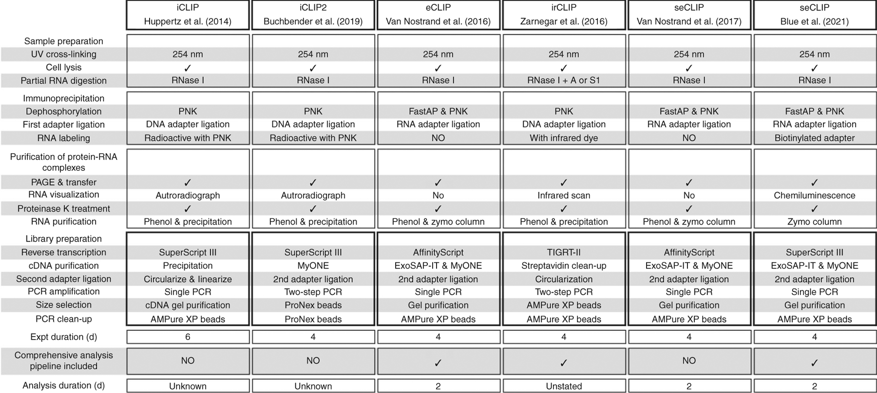
Comparison of seCLIP experimental and analysis workflow to iCLIP, iCLIP2, eCLIP, irCLIP and a previously published version of seCLIP. Expt, experiment; iCLIP, individual-nucleotide resolution cross-linking and IP; irCLIP, infrared-CLIP. Figure adapted with permission from ref.¹⁷, Elsevier.

Applications of the method

Most of the work using the standardized eCLIP and seCLIP methods has been performed in K562, HepG2 and HEK293T cell lines, but the highly adaptable nature of the method lends itself to many other cell types and tissues^9,29–34. Expanding seCLIP into new cell types or tissues often requires optimization, especially when it comes to RNA fragmentation. We have observed that for cell types or tissues that have moderate to high endogenous RNase activity (such as stem cells, neurons and many tissues), it is essential to add RNase inhibitor during the initial lysis step to prevent RNA over-fragmentation. In addition to timing, the amount of RNase inhibitor added may need to be increased, or RNase concentration decreased, for material with particularly high RNase activity. Lastly, the amount of overall RNA differs between cell types, and optimizing the RNase digestion enhances data quality.

In addition to identifying RNA-binding sites, CLIP has been used to study a number of epitranscriptomic modifications of RNA^35–37. Furthermore, eCLIP has been adapted to map RNA modifications such as N¹-methyladenosine (m1A) and N⁶-methyladenosine (m6A) in functional analyses of epitranscriptomic regulation by RBPs^38,39. Given the breadth of known RNA modifications and their connections to human disease, seCLIP has potential for exploring the mechanisms by which RBPs control these disease-related modification processes⁴⁰.

Experimental design

A description of the main steps in the seCLIP experimental protocol, including suggested and necessary controls, is provided below, and an overview is shown in Fig. 2.

Fig. 2 |. Overview of the seCLIP protocol.

a, UV cross-linking of cultured cells or tissue (Steps 1–4). b, Cells are lysed, and RNA is partially digested (Steps 8–11). c, The target protein is purified by using antibody-coupled magnetic beads (Step 12). d, RBP-RNA complexes are washed and dephosphorylated, enabling ligation of the 3′ linker (Steps 13–22). e, RBP-RNA complexes are denatured from beads and separated by SDS-PAGE, followed by transfer to nitrocellulose and PVDF membranes (Steps 23–27). IP success is visualized via western blot (Steps 28–31), and RBP-RNA complexes can be visualized via RNA biotinylation and streptavidin-HRP (Box 1). Western blot is used as a guide to isolate regions corresponding to RBP-bound RNA fragments. f, RNA is extracted from the membrane via proteinase digestion, SMInput RNA undergoes dephosphorylation and 3′ linker ligation and RNA is converted to cDNA by reverse transcription (Steps 32–56). g, RNA is degraded, and cDNA is purified (Steps 57–59). h, A UMI-containing linker is ligated to the 3′ end of cDNA molecules, followed by cleanup (Steps 60–65). i, cDNA libraries are quantified by qPCR, PCR-amplified and purified before quantification (Steps 66–82). j, Schematic of the final seCLIP library fragment. The unique molecular identifier is displayed in brown and labeled as UMI on the diagram.

UV cross-linking (Steps 1–4; Fig. 2a)

Cross-linking of cells and tissues with UV is generally straightforward. There is some flexibility when it comes to cell density during cross-linking, but we generally aim for 6 million cells/ml for suspension cells and 70–90% confluency for adherent cells. For tissues, cryogrinding and UV cross-linking frozen tissue powder has yielded successful eCLIP⁴¹, although great care must be taken to keep all tools chilled on dry ice or liquid nitrogen, because tools that have warmed will cause frozen tissue to thaw, making it hard to manipulate and encouraging RNA and protein degradation. Once irradiated, cell pellets or tissues can be kept at −80 °C without significant quality degradation.

For pilot experiments, we recommend preparing a non-irradiated control sample to run through the RNA visualization procedure (Box 1), which should show significantly decreased RNA (indicating cross-link dependency of the RBP-RNA interaction). Although libraries can be prepared from uncross-linked samples, the low RNA yield leads to poor library complexity, and thus we have found that libraries from SMInput samples are preferable for normalization.

Box 1 |. Cross-linked RNA visualization with biotin labeling 3 d.

RNA visualization can be used to verify three things: (i) that samples have been successfully cross-linked, (ii) that immunoprecipitated RNA migrates at the size of the RBP of interest in a high-RNase-digested sample and (iii) that the RNA present in the IP is cross-link-dependent. These steps can be done as a pilot experiment, done alongside the CLIP experiment if the overlapping workload is manageable or completed afterward.

Procedure.

1. In an RNase-free 1.5-ml microcentrifuge tube, mix the following reagents per sample:

   Component	Amount (μl)	Final
   H2O	9.6	-
   10× RNA ligase buffer (no DTT)	3.0	1.1×
   0.1 M ATP	0.3	1.1 μM
   100% DMSO	0.9	3.4%
   1% (vol/vol) Tween-20	0.6	0.022%
   50% (wt/vol) PEG 8000	9.0	17%
   Murine RNase inhibitor	0.4	0.8 U
   RNA ligase high-concentration enzyme	2.4	72 U
   Biotinylated cytidine (bis)phosphate	0.5	18.7 nM
   Total	26.7	-

2. Magnetically separate each reserved IP sample from Step 18, remove wash buffer and resuspend the beads in 26 μl of master mix.

3. Incubate samples at 16 °C with gentle shaking for 2 h or overnight (recommended).

4. Add 200 μl of cold high-salt wash buffer, mix, magnetically separate and remove the supernatant.

5. Add 500 μl of cold high-salt wash buffer, move on the magnet, add 500 μl of cold wash buffer and remove the supernatant.

6. Wash three times with 500 μl of cold wash buffer.

7. Resuspend in 20 μl of wash buffer.

8. Add 10.5 μl of denaturing mix for SDS-PAGE (7.5 μl of 4× LDS buffer and 3 μl of 1 M DTT).

9. Incubate at 70 °C, mixing at 1,200 rpm for 10 min.

10. Place tubes on ice for >1 min.

11. Magnetically separate samples and load 15 μl on a NuPAGE 4–12%, Bis-Tris, 10- or 12-well gel, reserving the other half at −20 °C as backup.

12. Run the gel at 150 V for 75 min.

13. Transfer to a nitrocellulose membrane at 30 V overnight.

14. Develop the membrane as follows by using the chemiluminescent nucleic acid detection module kit (cat. no. 89880):

    1. Slowly warm the blocking buffer and the 4× wash buffer to 37–50 °C in a water bath until all particulates are dissolved.
    2. Block the membrane by adding 10 ml of blocking buffer and incubate for 15 min with gentle shaking at room temperature (all further steps are done at room temperature).
    3. Prepare conjugate/blocking buffer solution by adding 31.25 μl of the stabilized streptavidin-HRP conjugate to 10 ml of blocking buffer.
    4. Decant blocking buffer from the membrane and add 10 ml to the conjugate/blocking solution. Incubate the membrane in the conjugate/blocking buffer solution for 15 min with gentle shaking.
    5. Prepare 1× wash solution by adding 40 ml of 4× wash buffer to 120 ml of water.
    6. Transfer the membrane to a new container and rinse briefly with 20 ml of 1× wash solution.
    7. Wash the membrane four times for 5 min each in 20 ml of 1× wash solution with gentle shaking.
    8. Transfer the membrane to a new container and add 30 ml of substrate equilibration buffer. Incubate the membrane for 5 min with gentle shaking.
    9. Prepare chemiluminescent substrate working solution by adding 2 ml of luminol/enhancer solution to 6 ml of stable peroxide solution. Note: Working solution is susceptible to damage via prolonged light exposure. Keep the solution in an amber bottle or keep it away from light.
    10. Remove the membrane from the substrate equilibration buffer and remove excess buffer. Place the membrane in a clean container or clean sheet of plastic wrap.
    11. Pour the substrate working solution onto the membrane so that it completely covers the surface. Incubate the membrane in the substrate solution for 5 min without shaking.
    12. Remove the membrane from the working solution and remove excess buffer. Do not allow the membrane to dry out.
    13. Wrap the membrane in plastic wrap, avoiding bubbles, and place in a film cassette. Obtain optimal signal by adjusting film exposure time or by exposing the membrane to multiple films simultaneously.

RNA fragmentation (Step 11; Fig. 2b)

Fragmentation of RNA transcripts is crucial for allowing precise mapping of RBP-binding sites after alignment, as well as limiting RNA-dependent co-purification of other RBPs. Our RNase conditions have proven to be applicable for many RBPs in multiple cancer cell lines, but we recommend doing a titration experiment as confirmation of optimal RNA fragment length (40–50 nt) for new cell lines or tissues of study, because over-digestion can lead to poor experimental yields and lack of peak signal^9,16. This optimization can be performed by digesting RNA from known amounts of lysed material with a range of RNase conditions and assessing fragment size distribution in a number of ways: (i) by using the RNA visualization method herein, (ii) radioactive labeling of fragments followed by electrophoresis and northern blotting and (iii) capillary electrophoresis such as a TapeStation or Bioanalyzer. It is recommended to use RBP-targeting antibodies that have already been profiled via (s)eCLIP when optimizing RNase digestion conditions in a new biological context, to mitigate uncertainty caused by using untested materials.

Immunoprecipitation of RBP complexes (Step 12; Fig. 2c,d)

This step is likely to require the most optimization and is critical to ensuring experimental success, especially if working with RBPs not previously profiled. Some key points to keep in mind include the following:

• Antibody selection. Traditional seCLIP relies on the use of an antibody capable of specifically and robustly reacting with its target protein in lysate. A simple IP-western test can be done to assess whether an antibody is capable of pulling down and detecting the protein of interest. Ideally, the same antibody would be useful for confirming IP success and efficiency via western blot, but in some cases a second antibody must be used at the western blot stage, because the initial antibody may not recognize both the native and denatured protein. Similarly, although monoclonal antibodies have high specificity for their targets and can result in lower background, polyclonal antibodies can be more likely to successfully immunoprecipitate because they bind to multiple epitopes on target proteins (but may require more careful validation with orthogonal experiments to ensure the lack of other co-immunoprecipitated RBPs).

• Controls. Paired control samples serve two purposes in seCLIP: to validate that the immunoprecipitated RNA is due to cross-linking to the RBP of interest and to provide a reference for quantitative identification of enriched regions. Paired samples in which the RBP of interest is knocked out provide the best control for the former, because they explicitly test whether the observed signal is dependent on the RBP of interest (however, we note that knockdown samples are typically not sufficient for this purpose, because immunoprecipitation of remaining expressed RBP may give lower overall RNA yield but often yield signal tracks similar to wild type after additional PCR amplification). CLIP using a nonspecific, isotype-matched (IgG) antibody can similarly be performed to determine the specificity of the RBP-specific CLIP. However, we have found that libraries made from these samples are often ill suited for quantification of enrichment because they can yield extremely low library yields (that are highly PCR-duplicated). We have found that using the SMInput instead captures similar information but provides sufficient yield to give informative read density tracks for normalization, and we recommend this as a standard control for every experiment.

SDS-PAGE and membrane transfer (Steps 23–27; Fig. 2e)

Performing SDS-PAGE on the RBP-RNA complexes is important for two reasons. First, it separates the target complexes from co-precipitated complexes that persist through the IP, enzymatic steps and washes. Second, the transfer to nitrocellulose membrane is posited to remove any free RNA molecules that likewise remain after the IP, enzymatic steps and washes¹⁶.

RNA pulldown visualization (Box 1; Fig. 2e)

In this protocol, protein-RNA complexes are visualized by ligation of a biotinylated oligo to bound RNA and then detected with an HRP-linked streptavidin. In this way, users can recapitulate the radioactive labeling of RNA found in previous CLIP protocols while avoiding the procedural challenges that accompany working with radioactivity (Fig. 2). By using high- and low-concentration RNase digestion and UV cross-linked and non-cross-linked cell pellets, users can confirm both RBP specificity and cross-link dependency of RNA binding in this single assay.

Library preparation and amplification (Steps 32–82; Fig. 2f–j)

After purification, RNA fragments undergo a series of enzymatic modifications in preparation for sequencing. Specifically, they are modified with adapters that enable reverse transcription (RT), allow for amplification and ultimately sequencing. The primary concerns during the library preparation process are (i) limiting degradation or loss of sample, (ii) reducing library overamplification and (iii) avoiding sample contamination.

To limit degradation by nucleases (particularly RNases), we recommend keeping tubes and bottles closed as much as possible and limiting airflow over tubes while they are open. Work surfaces should be cleaned routinely with an RNase-inactivating solution, and certified nuclease-free solutions and plasticware should be used throughout. Buffers should be remade often to ensure sterility, and any that are suspected of contamination should be discarded and replaced. Because seCLIP has many steps, the potential for cumulative sample loss cannot be ignored. Bead and column clean-up steps, although highly efficient, can lead to suboptimal sample recovery if not done carefully.

We use qPCR to determine the number of PCR cycles necessary to obtain a sequenceable library. This helps to ensure required amplification but avoid PCR artefacts caused by depletion of essential reagents that can lead to concatemer products and inaccurate library quantification. As might be expected, the optimal number of amplification cycles is highly RBP specific, where RBPs with lower cross-linked RNA yields will require more PCR cycles and have higher PCR duplication rates and fewer usable sequencing reads⁹.

Perhaps the most critical consideration for library preparation is avoiding sample contamination, particularly of adapter-containing PCR products. These contaminants are highly stable, and the introduction of even small amounts can lead to the identification of false-positive RBP binding sites on analysis. As such, we recommend having separate physical spaces for pre-amplification and post-amplification work in addition to doing frequent and regular cleanings of equipment and surfaces with 5–10% (vol/vol) bleach, followed by 70% (vol/vol) ethanol. Another type of potential contamination is from the accidental introduction of outside RNA molecules. RNA introduced before linker ligation can easily be carried through and can lead to false identification of RBP binding sites. The introduction of linker-containing RNA before RT can lead to a similar outcome. To identify this form of contamination and cross-contamination during large-scale experimentation, barcoded RNA linkers can be used to filter out RNA molecules not originating from a given experiment during analysis⁹.

Bioinformatic analysis

Once the (s)eCLIP library has been sequenced, bioinformatics analysis is used to quantify read enrichment, identify significant enriched peaks, and assess the overall quality of the experiment (Fig. 3). Below we outline several automated analyses as well as recommend quantitative metrics that can be used to assess the quality of an eCLIP dataset. For each step within the analyses, we define both the tool environment (i.e., software, version and dependencies) and the tool or workflow usage (i.e., command-line arguments and hardware requirements) by using Docker containers and Common Workflow Language (CWL), respectively. Docker is a container technology used here to simplify installation and deployment of required software, while CWL is a YALM (‘yet another markup language’)-based standard for defining how software is used within the context of an analysis pipeline.

Fig. 3 |. Overview of the eCLIP bioinformatics workflow.

a, Outline of steps used to call significantly enriched peaks from fastq files as well as derive quality control metrics such as the number of usable reads and entropy total across peaks. b, Intermediates taken from the peak calling workflow may be used to discover bound repetitive elements. c, Irreproducibility discovery rate (IDR) may be used to merge two replicate sets of peaks and compute rescue and self-consistency ratios to be used to evaluate irreproducibility.

Description of automated workflows

Basic analysis of eCLIP data can be described with three distinct workflows, which as designed will improve the robustness of our pipeline toward different experimental setups.

The first uses uniquely mapped reads to generate a list of candidate binding sites (peaks). We consider this the ‘core pipeline’ because this workflow serves as the starting point for most eCLIP analyses, using fastq files taken from the sequencer as the initial input. Briefly described, IP and SMInput reads generated from the seCLIP protocol are first extracted of their UMIs and adapter-trimmed to improve mappability. Reads are then mapped to a curated list of repeat elements, with only unmapped reads kept and mapped to a genome of interest. After mapping, PCR duplicates (defined as reads that map to the same location and have the same UMI sequence) are removed. The remaining ‘usable reads’ (uniquely mapped, PCR-deduplicated fragments) are used as inputs to a peak caller (CLIPper) to identify clusters of locally enriched read density. Reads originating from the IP are then compared to SMInput reads within these coordinates to identify peaks that are significantly enriched above background.

The second ‘merging replicates and assess irreproducibility’ pipeline uses replicate datasets to identify reproducible peaks. In this analysis, SMInput-normalized peaks from the first pipeline are ranked according to information content: $p_i*{\text{log}}_{\text{2}}\frac{p_i}{q_i}$ where p_i and q_i are the respective number of IP and SMInput reads within each peak divided by the corresponding total number of uniquely mapped non-PCR duplicate reads and are used as inputs to generate a single list of reproducible binding sites. This pipeline also computes rescue and self-consistency ratios, which are quantitative metrics that can be used to gauge reproducibility in both ChIP-seq and CLIP-seq experiments^29,42.

A third workflow was developed to use intermediates from the first pipeline to determine RBP enrichments at repeat families and other multi-copy elements¹¹. Designed as an orthogonal approach to peak calling, this pipeline maps trimmed fastq files to a set of 8,108 manually curated sequences belonging to distinct repeat families, including ribosomal RNAs (e.g., 18S, 28S, 5S, 5.8S and the 45S precursor), small nuclear RNAs (snRNAs; e.g., U1 and U2), small nucleolar RNAs (snoRNAs), tRNAs, Ro-associated Y RNAs (YRNAs) and repetitive elements (e.g., Alu, long interspersed nuclear elements and endogenous retroviruses (ERVs). It then merges these repeat-mapped reads with genome-mapped reads and performs its own PCR-deduplication step, resulting in a table of enriched binding sites within repeat families or unique genomic elements.

Description of QC metrics

Accurate-extrapolated cycle threshold (C_T) (a-eC_T).

Successful recovery of a significant number of unique RNA fragments in the final eCLIP library is a key benchmark of experimental success. Although a minimum for the number of unique RNA fragments recovered (reflected as the number of non-PCR duplicate reads) is empirically determined during data processing above, we developed the a-eC_T metric to estimate this recovery during the eCLIP experimental procedure itself. a-eC_T is defined as the number of PCR cycles necessary to obtain 100 fmol of amplified library (10 ul of 10 nM, a standard starting amount for sequencing) by using an experimentally derived 1.84-fold amplification per cycle²⁹. This metric enables rapid comparison of experimental yield versus negative controls (IgG isotype or RBP knockout samples) and can be used to estimate the total number of unique RNA molecules contained within the library with reasonable accuracy²⁹.

Minimum usable read number.

Although usable read number can depend on the number of sequenced reads and vary among successful eCLIP experiments, manual curation found that most passable ENCODE eCLIP datasets (439/446) contained ≥1.5 million usable read fragments, whereas non-passable datasets were several times more likely to contain less²⁹. As such, this cutoff can serve as a general recommendation for identifying likely unsuccessful experiments that should be subjected to careful inspection. However, we note that it is possible to generate high-quality data that do not meet this threshold (especially for RBPs with low abundance and a small number of targets).

Information content.

A high-quality eCLIP dataset should contain significantly enriched signal above SMInput. To quantify this, we defined the sum of relative information across all peaks as a metric that incorporates both the number of and enrichment at all peaks for an eCLIP dataset. This information content metric showed high accuracy, particularly indicating datasets with little enriched signal²⁹.

Reproducibility across replicates.

As good practice, we recommend that experimental designs include replicates to ensure that biological findings are minimally reproducible. To quantify this, we incorporated the irreproducible discovery rate (IDR) approach previously described for ChIP-seq data analysis, which uses downsampled pseudo-replicates to query whether the two replicates show better reproducibility than expected by chance⁴³. Using the same criteria as previously used for transcription factor ChIP-seq, we define a passing dataset as one where the rescue ratio and self-consistency ratios are both >2, a borderline dataset as one where only one of the two ratios is >2 and a failed dataset if both are <2. These criteria showed significant predictive power when tested on manually curated datasets²⁹ and enable a standard assessment of broad data reproducibility.

Expertise needed to implement the protocol

Although the seCLIP method incorporates a wide range of molecular biology techniques, it does not require any special expertise to perform. However, because this is an RNA-based method, general care must be taken to avoid sample degradation by RNases and cross-contamination, as outlined above. Sequencing of seCLIP libraries can be performed on Illumina high-throughput sequencing platforms (NextSeq, HiSeq or NovaSeq) with standard reagents and protocols.

We have provided a single instance implementation of our bioinformatics workflows that require only basic knowledge of running terminal commands and of Amazon’s EC2 services. However, we expect end users to have a technical understanding of their own computing environments because they may vary among institutions. This includes the ability to install the requisite software or the ability to run containers made available through Dockerhub or Singularity. In particular for scaled multi-instance high-performance computing (HPC) environments, end-users must install a framework (e.g., Toil⁴⁴) capable of submitting jobs to the system’s resource manager (e.g., Portable Batch System (PBS) and Slurm) on the pipeline’s behalf. Users must also ensure that their environment meets the storage and memory requirements, which are defined within each step of the provided CWL documents.

Limitations

The primary limitation with the seCLIP method is the availability of IP-grade antibodies, a common limitation of any IP-based approach. Profiling endogenous factors is always preferred, because exogenous expression levels of an RBP may disrupt the binding kinetics or stoichiometry of RNA binding. However, screening for suitable antibodies against one or more targets can be costly and is often met with irregular success. To facilitate this effort, we performed a large-scale screen in K562 cells to find RBP-specific, IP-compatible antibodies, ultimately identifying antibodies against 365 RBPs⁴⁵. However, many less well-characterized factors still have no commercially available antibodies. In these cases, the use of peptide tags (whether added to RBP open reading frame transgenes or integrated into the endogenous RBP loci via CRISPR–Cas9–mediated integration) can enable seCLIP studies to be performed, and IP-validated antibodies are commercially available for many standard tags³¹. However, in these cases, caution must be taken to validate that the tag does not interfere with RBP binding or function.

Materials

Biological materials

• Hep-G2 cell line (American Type Culture Collection, cat. no. HB-8065; RRID: CVCL_0027)

• K562 cell line (American Type Culture Collection, cat. no. CCL-243; RRID: CVCL_0004) The cell lines used in your research should be regularly checked to ensure that they are authentic and are not infected with mycoplasma.

Reagents

• Pure, nuclease- and nucleic acid–free water (such as MilliQ)

• Molecular biology grade water (Corning, cat. no. 46–000-CM)

• DMSO (Sigma-Aldrich, cat. no. D2650)

• Dulbecco’s PBS (DPBS), 1×, without calcium and magnesium (Corning, cat. no. 21–031-CV)

• Tris-HCl pH 7.4, 1 M stock solution (Teknova, cat. no. T1074)

• Sodium chloride, 5 M stock solution (Lonza, cat. no. 51202)

• Igepal CA-630 (Sigma-Aldrich, cat. no. I8896)

• SDS, 10% (wt/vol) solution (Lonza, cat. no. 51213)

• Sodium deoxycholate (Sigma-Aldrich, cat. no. D6750) Sodium deoxycholate powder is harmful if swallowed and irritating if inhaled. Use inside a fume hood.

• EDTA, 0.5 M solution (Sigma-Aldrich, cat. no. E7889)

• Magnesium chloride, 1 M solution (Invitrogen, cat. no. AM9530G)

• Tween-20, for seCLIP buffers (Sigma-Aldrich, cat. no. P9416)

• Tween-20, for TBST buffer (Sigma-Aldrich, cat. no. P1379)

• Ethanol, 100% and 80% (vol/vol) stocks (Sigma-Aldrich, cat. no. E7023) Ethanol is flammable.

• Isopropanol, 100% (Fisher Scientific, cat. no. A416–500)

• RLT buffer (Qiagen, cat. no. 79216)

• Hydrochloric acid, 1 N solution (Fisher Scientific, cat. no. SA48500) 1 N hydrochloric acid causes skin irritation.

• Sodium hydroxide, 1 N solution (Fisher Scientific, cat. no. S25549) 1 N sodium hydroxide causes skin irritation.

• Turbo DNase, 2 U/μl (Invitrogen, cat. no. AM2239)

• RNase I, 100 U/μl (Invitrogen, cat. no. AM2295)

• FastAP thermosensitive alkaline phosphatase, 1 U/μl (Thermo Scientific, cat. no. EF0652)

• RNase inhibitor, murine, 40 U/μl (New England BioLabs, cat. no. M0314L)

• T4 polynucleotide kinase, 10 U/μl (New England BioLabs, cat. no. M0201L)

• T4 RNA ligase 1 (ssRNA ligase, high concentration, 30 U/μl (New England BioLabs, cat. no. M0437M)

• Biotinylated cytidine (bis)phosphate (pCp-Biotin; Jena Bioscience, cat. no. NU-1706-BIO)

• Proteinase K, molecular biology grade, 0.8 U/μl (New England BioLabs, cat. no. P8107S)

• 5′ Deadenylase, 50 U/μl (New England BioLabs, cat. no. M0331S)

• Q5 high-fidelity 2× master mix (New England BioLabs, cat. no. M0492L)

• Protease inhibitor cocktail III (EMD Millipore, cat. no. 539134)

• SuperScript III reverse transcriptase, 200 U/μl (Invitrogen, cat. no. 18080044)

• ExoSAP-IT PCR product cleanup reagent (Applied Biosystems, cat. no. 78201.1.ML)

• Dynabeads M-280 sheep anti-rabbit IgG, 10 mg/ml (Invitrogen, cat. no. 11204D)

• Dynabeads M-280 sheep anti-mouse IgG, 10 mg/ml (Invitrogen, cat. no. 11202D)

• Dynabeads MyOne silane, 40 mg/ml (Thermo Fisher Scientific, cat. no. 37002D)

• PowerSYBR green PCR master mix (Applied Biosystems, cat. no. 4367659)

• Agencourt, AMPure XP (Beckman Coulter, cat. no. A63881)

• NuSieve GTG agarose (Lonza, cat. no. 50084)

• SYBR Safe DNA gel stain (Invitrogen, cat. no. S33102)

• 50-bp DNA ladder (Invitrogen, cat. no. 10416014)

• NuPAGE LDS sample buffer, 4× (Invitrogen, cat. no. NP0008)

• DL-Dithiothreitol (Sigma-Aldrich, cat. no. D9779)

• MOPS SDS running buffer, 20× (Invitrogen, cat. no. NP0001)

• NuPAGE transfer buffer, 20× (Invitrogen, cat. no. NP00061)

• NuPAGE 4–12%, Bis-Tris protein gels, 1.5 mm, 10 wells (Invitrogen, cat. no. NP0335BOX)

• NuPAGE 4–12%, Bis-Tris protein gels, 1.0 mm, 12 wells (Invitrogen, cat. no. NP0322BOX)

• Spectra multicolor broad-range protein ladder (Thermo Scientific, cat. no. 26623)

• Nonfat dry milk (Genesee Scientific, cat. no. 20–241)

• RNA-binding protein-targeting antibody, for immunoprecipitation (varies by experiment)

• Mouse TrueBlot ULTRA anti-mouse Ig HRP antibody (Rockland Immunochemical, cat. no. 18–8817-33; RRID: AB_2610851)

• Rabbit TrueBlot anti-rabbit Ig HRP antibody (Rockland Immunochemical, cat. no. 18–8816-33; RRID: AB_2610848)

• Anti-TIAL1 antibody (MBL International, cat. no. RN059PW; RRID: AB_10794609)

• Anti-PRPF39 antibody (Thermo Fisher Scientific, cat. no. PA5–21627; RRID: AB_11154431)

• 10× TBS, made from Trizma base (Sigma-Aldrich, cat. no. T6066) and sodium chloride (Fisher Scientific, cat. no. S271–10), pH 7.6 with hydrochloric acid (Fisher Scientific, cat. no. A144–212)

• D1000 ScreenTape (Agilent Technologies, cat. no. 5067–5582)

• D1000 reagents (Agilent Technologies, cat. no. 5067–5583)

RNA oligo

• InvRiL19: /5Phos/rArGrArUrCrGrGrArArGrArGrCrArCrArCrGrUrC/3SpC3/ (Order 100 nmol of RNA oligo, standard desalting; storage stock: 200 μM; working stock: 40 μM; final concentration: 1 μM (SMInput), 4 μM (CLIP).)

DNA oligos

• InvRand3Tr3: /5Phos/NNNNNNNNNNAGATCGGAAGAGCGTCGTGT/3SpC3/ (Order 100 nmol of DNA oligo, standard desalting; storage stock: 200 μM; working stock: 80 μM; final concentration: 3 μM.)

• InvAR17: CAGACGTGTGCTCTTCCGA (Order 25 nmol of DNA oligo, standard desalting; storage stock: 200 μM; working stock: 20 μM; final concentration: 0.5 μM.)

• D501_qPCR: AATGATACGGCGACCACCGAGATCTACACTATAGCCTACACTCTTTCCCTACACGACGCTCTTCCGATCT

• D701_qPCR: CAAGCAGAAGACGGCATACGAGATCGAGTAATGTGACTGGAGTTCAGACGTGTGCTCTTCCGATC (For qPCR use, we typically order these oligonucleotides without additional purification.)

PCR primers

For each, order 1 μmol, PAGE purification; storage stock: 100 μM; working stock: 20 μM; final concentration: 1 μM.

• PCR_F_D501: AATGATACGGCGACCACCGAGATCTACACTATAGCCTACACTCTTTCCCTACACGACGCTCTTCCGATCT

• PCR_F_D502: AATGATACGGCGACCACCGAGATCTACACATAGAGGCACACTCTTTCCCTACACGACGCTCTTCCGATCT

• PCR_F_D503: AATGATACGGCGACCACCGAGATCTACACCCTATCCTACACTCTTTCCCTACACGACGCTCTTCCGATCT

• PCR_F_D504: AATGATACGGCGACCACCGAGATCTACACGGCTCTGAACACTCTTTCCCTACACGACGCTCTTCCGATCT

• PCR_F_D505: AATGATACGGCGACCACCGAGATCTACACAGGCGAAGACACTCTTTCCCTACACGACGCTCTTCCGATCT

• PCR_F_D506: AATGATACGGCGACCACCGAGATCTACACTAATCTTAACACTCTTTCCCTACACGACGCTCTTCCGATCT

• PCR_R_D701: CAAGCAGAAGACGGCATACGAGATCGAGTAATGTGACTGGAGTTCAGACGTGTGCTCTTCCGATC

• PCR_R_D702: CAAGCAGAAGACGGCATACGAGATTCTCCGGAGTGACTGGAGTTCAGACGTGTGCTCTTCCGATC

• PCR_R_D703: CAAGCAGAAGACGGCATACGAGATAATGAGCGGTGACTGGAGTTCAGACGTGTGCTCTTCCGATC

• PCR_R_D704: CAAGCAGAAGACGGCATACGAGATGGAATCTCGTGACTGGAGTTCAGACGTGTGCTCTTCCGATC

• PCR_R_D705: CAAGCAGAAGACGGCATACGAGATTTCTGAATGTGACTGGAGTTCAGACGTGTGCTCTTCCGATC

• PCR_R_D706: CAAGCAGAAGACGGCATACGAGATACGAATTCGTGACTGGAGTTCAGACGTGTGCTCTTCCGATC

Equipment

• Tissue culture dishes (100 or 150 mm for culturing and cross-linking) and flasks (T225 for culturing)

• Conical tubes, 15 and 50 ml

• PCR tubes, 0.2 ml

• DNA LoBind microfuge tubes, 1.5 ml (Eppendorf, cat. no. 022431021)

• 384-well qPCR plates (Bio-Rad, cat. no. HSP3801)

• UV cross-linker (254 nm; CL-1000 from UVP/Analytik Jena)

• Centrifuge suitable for 15- and 50-ml conical tubes (to pellet cells)

• Freezers (−20 °C and −80 °C for storing enzymes, buffers, oligos and cell pellets)

• Metal block, sized to fit inside cross-linker (optional), for keeping cells cold during cross-linking

• Microcentrifuge (refrigerated)

• End-over-end microcentrifuge tube rotator

• Water bath sonicator (such as Bioruptor Plus, B01020004, from Diagenode)

• DynaMag-2 magnet (Thermo Scientific, cat. no. 12321D)

• 96-well magnetic separator (such as MagWell Separator 96; EdgeBio, cat. no. 57624)

• RNA clean and concentrator-5 kit (Zymo Research, cat. no. R1016)

• Chemiluminescent nucleic acid detection module (optional) (Thermo Scientific, cat. no. 89880)

• Pierce enhanced chemiluminescence (ECL) western blotting substrate (Thermo Scientific, cat. no. 32106)

• Darkroom with autoradiography film developer

• Autoradiography film (such as ProSignal blotting film; Genesee Scientific, cat. no. 30–810L)

• Cold room

• Physically separate locations for working with pre-amplification and post-amplification materials

• Vortex machine

• Benchtop rocker

• Plastic wrap

• Sheet protectors

• Autoradiography cassette

• Sterile razor blades

• Tweezers

• Western blotting trays

• Microscope slides, for chopping nitrocellulose membranes (such as cat. no. 12–550-343 from Fisher Scientific)

• Glass plate (optional) or other hard, cleanable surface for cutting out membrane slices

• Positive displacement pipette (optional) (such as MR-250 from Rainin)

• Temperature-controlled microcentrifuge tube shaker (such as Eppendorf ThermoMixer R or ThermoMixer C)

• Vertical gel electrophoresis apparatus (such as XCell SureLock Mini-Cell system, Thermo Scientific)

• Mini Trans-Blot cell blotter (Bio-Rad, cat. no. 17039300)

• PowerPac power supply (Bio-Rad, cat. no. 1645050 or 1645052)

• PowerPac adaptor (Bio-Rad, cat. no. 1645064)

• Nitrocellulose blotting membrane, 0.45 μm (GE Healthcare, cat. no. 10600007)

• PVDF blotting membrane, 0.45 μm (EMD Millipore, cat. no. IPFL00010)

• Whatman paper, 3MM grade (GE Healthcare, cat. no. 3030–917)

• Filter roll, for use as disposable sponges during western blotting (Grainger, cat. no. 6U592)

• Thermal cycler (such as the Bio-Rad T100)

• Access to a 384-well qPCR machine (such as the CFX384 Touch Real-Time PCR detection system; Bio-Rad, cat. no. 1855485)

• Horizontal gel electrophoresis apparatus (such as the Mini-Sub Cell GT electrophoresis system (Bio-Rad, cat. no. 1704466) or the Wide Mini-Sub Cell GT electrophoresis system (Bio-Rad, cat. no. 1704405))

• Blue light transilluminator (to visualize SYBR Safe–stained gels)

• MinElute gel extraction kit (Qiagen, cat. no. 28606)

• Agilent 2200 TapeStation (to quality check and quantify sequencing library)

• Access to high-throughput sequencing (the primers used in this protocol are designed to work for HiSeq & NovaSeq Illumina sequencing platforms)

• Access to at least one high-performance compute node running Linux with at least 8 cores and 32 GB of memory. All of our data processing is done on an HPC cluster, using 24 nodes each with 16 (2.6-GHz Intel Xeon E5–2670) processors and 126 Gb of memory, operating on Centos 7 and using PBS Torque job scheduling software.

Reagent setup

We prepare the following buffers by using nuclease-free buffer stock solutions previously listed in Reagents and bringing them up to the final volume by using molecular biology–grade water. Detergents (Tween-20, Igepal and sodium deoxycholate) are prepared as 5–10% stock solutions (Tween-20, vol/vol; Igepal, vol/vol; sodium deoxycholate, wt/vol) in molecular biology–grade water and diluted appropriately during buffer preparation. Avoiding nuclease and nucleic acid contamination of all buffers is essential, and replacement of buffers every few months is good practice to maintain quality.

Lysis buffer

Lysis buffer contains 50 mM Tris-HCl pH 7.4, 100 mM NaCl, 1% (vol/vol) Igepal CA-630, 0.1% (vol/vol) SDS and 0.5% (wt/vol) sodium deoxycholate. This buffer is stable at 4 °C for ≥6 months.

High-salt wash buffer

High-salt wash buffer contains 50 mM Tris-HCl pH 7.4, 1 M NaCl, 1% (vol/vol) Igepal CA-630, 1 mM EDTA, 0.1% (vol/vol) SDS and 0.5% (wt/vol) sodium deoxycholate. This buffer is stable at 4 °C for ≥6 months.

Wash buffer

Wash buffer contains 20 mM Tris-HCl pH 7.4, 10 mM MgCl₂, 0.2% (vol/vol) Tween-20 and 5 mM NaCl. This buffer is stable at 4 °C for ≥6 months.

RLTW buffer

RLTW buffer contains 1× RLT buffer and 0.025% (vol/vol) Tween-20. This buffer is stable at room temperature (20–25 °C) for ≥6 months.

10× PNK7 buffer

PNK buffer contains 700 mM Tris-HCl pH 7 and 100 mM MgCl₂. This buffer is stable at −20 °C for ≥6 months.

10× RNA ligase buffer (no DTT)

Ligase buffer without DTT contains 500 mM Tris-HCl pH 7.4 and 100 mM MgCl₂. This buffer is stable at −20 °C for ≥6 months.

PKS buffer

PKS buffer contains 100 mM Tris-HCl pH 7.4, 50 mM NaCl, 10 mM EDTA and 0.2% (vol/vol) SDS. This buffer is stable at room temperature for ≥6 months.

PCR elution buffer

PCR elution buffer contains 10 mM Tris-HCl pH 7.4, 20 mM NaCl and 0.1 mM EDTA. This buffer is stable at −20 °C for ≥6 months.

TT elution buffer

TT elution buffer contains 10 mM Tris-HCl pH 7.4, 0.1 mM EDTA and 0.01% (vol/vol) Tween-20. This buffer is stable at room temperature for ≥6 months.

Equipment setup

Software installation

Our pipeline (source code available at https://doi.org/10.5281/zenodo.5076591) is designed to run either on a single machine (locally or through a cloud provider such as Amazon Web Services) using the CWL reference implementation or any Toil-supported HPC (Torque, Grid Engine, Slurm or load-sharing facility (LSF)). In the Procedure, we provide instructions to implement all steps of the bioinformatics workflow (Steps 84–112). We also provide complete end-to-end tutorials (including installation) for running each pipeline (peak-calling, repeat family mapping, merging replicates and assessing irreproducibility) on the cloud via Amazon Web Services:

• Peak-calling pipeline (Steps 84–94)—GitHub: http://github.com/yeolab/eclip; tutorial: https://github.com/YeoLab/eclip/blob/master/documentation/Zero_to_peaks.pdf

• Repeat family mapping (Steps 95–99)—GitHub: https://github.com/yeolab/repetitive-element-mapping; tutorial: https://github.com/YeoLab/eclip/blob/master/documentation/Repeat_mapping.pdf

• Merging replicates and assessing irreproducibility (Steps 100–107)— GitHub: https://github.com/yeolab/merge_peaks; tutorial: https://github.com/YeoLab/eclip/blob/master/documentation/Reproducible_peaks.pdf

Procedure

Part 1: seCLIP

This protocol was developed as a part of the ENCORE (Encyclopedia of RNA Elements) project, which was designed to develop a map of functional RNA elements encoded in the human genome and their direct protein regulators. As such, the experimental setup outlined here was tailored to meet the guidelines and standards laid out by the consortium. Per ENCORE criteria, a full experiment includes four libraries: two seCLIP experiments on UV-cross-linked biological replicate samples and two SMInput control samples (taken from each of the cross-linked samples). The cell number and antibody/bead volumes used can be adjusted to fit experimental restrictions but may require optimization to ensure quality results.

Because this is an RNA-based assay, great care should be taken to avoid material degradation via nucleases, which can be achieved by wiping down work surfaces and equipment with 70% (vol/vol) ethanol and RNase decontamination solutions. In addition, DNase- and RNase-free consumables, good practices like closing tubes and bottles whenever possible and limiting breathing and moving over open tubes should be used throughout.

Sample preparation and UV cross-linking 1–2 hr

• 1For adherent cells, wash them once with DPBS and add enough cold DPBS to cover the cell monolayer. For suspension cells, spin down cells (200g for 5 min at room temperature) to pellet and aspirate the culture medium. Resuspend the cells in cold DPBS (3 ml for a 10-cm dish or 10 ml for a 15-cm dish) and transfer them to a clean dish. For frozen tissue, grind it well on liquid nitrogen and transfer the powder to a Petri dish on dry ice.
• 2Insert a shallow tray containing a layer of ice or a prechilled metal block into the cross-linker. Place the plates onto ice or a block and ensure that they are level. Remove the plate lids and cross-link the plates at 400 mJ/cm².

  For tissues, the plates and all tools should be kept on dry ice or liquid nitrogen throughout to prevent the tissue from thawing. Tissue should be cross-linked twice at 400 mJ/cm² with a brief redistribution of the powder between rounds.

• 3Once cross-linking is finished, transfer the cells from the plate to a conical tube or sterile bottle by pipetting suspension cells or scraping and then pipetting adherent cells. Wash each plate one time with DPBS to collect the remainder of the cross-linked cells and add them to the previously harvested cells. Tissue powder can be scooped directly into cold microcentrifuge tubes and kept at −80 °C until needed.
• 4Centrifuge harvested cells at 300g for 3 min at 4 °C. Aspirate the supernatant and resuspend the cell pellet in 1× DPBS to 20 million cells/ml or the desired concentration. Dispense the cell suspension into microcentrifuge tubes corresponding to the desired cell number and centrifuge at 300g for 3 min at 4 °C. Aspirate the supernatant and flash-freeze the cell pellets in liquid nitrogen.

  Cross-linked cells or tissue can be used immediately for lysis and IP or stored at −80 °C until use.

Bead preparation 1 h

• 5Chill lysis, high-salt wash and wash buffers in a cold room or on ice; all subsequent steps require chilled buffers. Distribute 125-μl aliquots, per IP replicate, of sheep anti-rabbit IgG or sheep anti-mouse IgG Dynabeads into clean microcentrifuge tubes.

  Make sure that the host species of your RBP-specific primary antibody matches the target species of the Dynabeads used (i.e., rabbit primary antibody with sheep anti-rabbit IgG Dynabeads).

• 6Magnetically separate the beads and remove the cleared supernatant, being careful not to disturb the bead pellet. Wash the beads two times in 500 μl of cold lysis buffer by moving the tube support rack to alternating sides of the magnet so that the beads move through the buffer. Avoid mixing by vortex because this may be too harsh. Remove the buffer and resuspend in 100 μl of lysis buffer per sample.
• 7Add 10 μg of RBP-specific antibody per IP sample to the washed beads and mix on an end-over-end tube rotator at room temperature for 45 min.

  10 μg is a suggested starting point appropriate for many antibodies, but the amount of antibody can be further optimized.

Cell lysis, RNase digestion and IP 3 h or overnight

• 8While the antibodies and beads are mixing, prepare lysis buffer by adding 5.5 μl of protease inhibitor cocktail III to 1 ml of cold lysis buffer per cell pellet being lysed.

  For tissues or cell types with high amounts of endogenous RNases, add 11 μl of murine RNase inhibitor per 1 ml of lysis buffer and protease inhibitor mixture. This works for embryonic stem cells, neuronal stem cells and many tissues but may need to be further increased for particularly difficult tissues (e.g., pancreas).

• 9Collect cross-linked cells from −80 °C storage and add 1 ml of cold lysis buffer + protease inhibitor mix to each pellet. Pipette up and down to resuspend until the pellet dissolves and the liquid is homogenous. Place tubes on ice and lyse for 5 min.
• 10Sonicate by using a Bioruptor on the low setting in a cold room for 5 min, cycling 30 s on and 30 s off. Place the tubes on ice.
• 11Dilute RNase I in DPBS at 1:25 on ice. To your lysed samples, add 5 μl of Turbo DNase and 10 μl of diluted RNase I, mix and immediately place in a Thermomixer preheated to 37 °C. Incubate for exactly 5 min, shaking at 1,200 rpm, and then place on ice. Immediately add 11 μl of murine RNase inhibitor (if added to lysis buffer earlier, ignore this). Centrifuge at 15,000g for 10 min at 4 °C.

  RNase I is sensitive to the SDS in the lysis buffer and loses activity after ~5 min, thus necessitating immediate incubation.

• 12While spinning down the lysates, wash the antibody + bead complexes from Step 7 two times in 500 μl of lysis buffer. After the final wash, spin down the tubes and then remove the remainder of the wash buffer. Transfer the cleared lysates to antibody-bound beads, being careful not to disturb the cellular debris pellet. Rotate at 4 °C for 2 h or overnight (recommended).

Dephosphorylation of IP samples 1 h

• 13Retrieve lysates from 4 °C and mix well by inversion. Transfer 20 μl of each lysate (including beads) into two clean tubes and store on ice until Step 23. These will serve as SMInput samples, one for the RNA preparatory gel and one for the diagnostic western blot. Optionally, you can also reserve 20 μl of ‘supernatant’ (magnetically cleared lysate) to assess the extent of target depletion during western blotting.
• 14Magnetically separate the remaining lysates and wash beads two times with 500 μl of high-salt wash buffer. Perform a transition wash by adding 500 μl of high-salt wash buffer, mixing and then adding 500 μl of wash buffer. Transition washes are done to minimize disruptions of antibody-RBP complexes due to abrupt changes in salt concentrations. Wash three times with 500 μl of wash buffer.
• 15
  Briefly spin the beads and remove residual wash buffer. Resuspend the beads in dephosphorylation master mix by gently flicking the tubes. Prepare the dephosphorylation mix in a microcentrifuge tube with the following components per sample:

  Component	Amount (μl)	Final
  H2O	38	-
  10× FastAP Buffer	5	1×
  Murine RNase inhibitor	2	80 U
  Turbo DNase	2	4 U
  FastAP enzyme	3	3 U
  Total	50	-

• 16
  Incubate the reaction in a Thermomixer at 37 °C, mixing at 1,200 rpm for 10 min. This step removes the 3′-cyclic phosphate group left behind by RNase I cleavage. While incubating, prepare the PNK master mix in a microcentrifuge tube with the following components per sample:

  Component	Amount (μl)	Final
  H2O	126	-
  10× PNK7 buffer	20	1×
  T4 PNK enzyme	4	40 U
  Total	150	-

• 17Without removing the dephosphorylation mix, add the PNK master mix and incubate the reaction in a Thermomixer at 37 °C, mixing at 1,200 rpm for 20 min. T4 PNK ensures that the RNA fragments are completely dephosphorylated on the 3′ end and are primed for 3′ adapter ligation.
• 18Add 200 μl of high-salt wash buffer, mix, magnetically separate beads and remove the supernatant. Transition to wash buffer by adding 500 μl of high-salt wash buffer, mix and add 500 μl of wash buffer. Remove the supernatant. Wash three times with 500 μl of wash buffer.

  (Optional) Before carrying out 3′ ligation in the next steps, reserve 10% of the IP samples for biotin labeling to visualize the RNA cross-linked to your RBP of interest (see Box 1 for further explanation).

3′ RNA adapter ligation of IP samples 2 h

• 19
  Prepare 3′ RNA adapter master mix in a microcentrifuge tube at room temperature with the following components per sample:

  Component	Amount (μl)	Final
  H2O	8.4	-
  10× RNA ligase buffer (no DTT)	3.0	1.2×
  0.1 M ATP	0.3	1.2 μM
  100% DMSO	0.9	3.6%
  1% (vol/vol) Tween-20	0.6	0.024%
  50% (wt/vol) PEG 8000	9.0	18%
  Murine RNase inhibitor	0.4	0.8 U
  T4 RNA ligase high-concentration enzyme	2.4	72 U
  Total	25	-

  The ligase buffer in this reaction contains no DTT, because we have observed that some antibodies are susceptible to presumed reduction by DTT, resulting in the loss of target RBP-RNA complexes. A positive displacement pipette, although optional, is very handy for pipetting viscous liquids like PEG 8000. Alternatively, pipette very slowly with a normal pipette tip.

• 20Briefly spin down beads from Step 18, add the 3′ RNA linker mix and 2.5 μl of InvRiL19 RNA adapter to each sample. Flick the tubes to mix, briefly centrifuge and incubate at room temperature, rotating end-over-end for 75 min.
• 21Wash beads in 500 μl of wash buffer, magnetically separate and remove the supernatant. Transition to high-salt wash buffer by adding 500 μl of wash buffer, mixing, adding 500 μl of high-salt wash buffer and mixing again. Magnetically separate and remove the supernatant, then add 500 μl of high-salt wash buffer and mix. Transition to wash buffer by removing the supernatant, adding 500 μl of high-salt wash buffer, mixing, adding 500 μl of wash buffer, mixing again and removing the supernatant. Wash two times with wash buffer.
• 22Remove the supernatant and briefly spin tubes. Remove the residual buffer, add 100 μl of wash buffer and mix. Transfer 20 μl from each bead sample to clean microcentrifuge tubes to serve as an IP sample for the diagnostic western blot. Magnetically separate the remainder of the beads, remove the supernatant, briefly spin and remove the remainder of the buffer. Add 20 μl of wash buffer to the beads, which will serve as the IP sample for the RNA preparatory gel.

SDS-PAGE and membrane transfers 3–4 h or overnight

• 23
  To each of your collected 20-μl SMInput and IP samples (two each of SMInputs and IPs for RNA gel, and two each of SMInputs and IPs for western blot), add a master mix of the following components:

  Component	Amount (μl)	Final (including sample)
  4× NuPAGE LDS buffer	7.5	0.98×
  1 M DTT	3.0	98 mM
  Total	10.5	-

• 24Flick each tube to mix, briefly spin and denature on a Thermomixer, shaking at 1,200 rpm at 70 °C for 10 min. Place on ice for >1 min.
• 25Briefly spin the SMInput and bead samples and magnetically separate them on ice. Load the supernatants on NuPAGE 4–12%, Bis-Tris, gels. We load half of the western blot samples and reserve the other half at −20 °C to be rerun, if needed.

  For RNA preparatory gels, load samples such that they are separated by a lane containing a small amount of protein ladder, which will serve as boundaries for cutting out membrane pieces after they are transferred. Western blot gels do not need these ladder boundaries.

• 26Run the gels in 1× MOPS SDS running buffer at 150 V at room temperature for 75 min, as per the manufacturer’s instructions. The run time may be adjusted on the basis of the size of the target protein.
• 27Transfer the RNA gels to a nitrocellulose membrane and western gels to methanol-activated PVDF by using a Bio-Rad mini trans-blot cell for 2 h at 200 mA or overnight at 30 V (preferred) in 1× MOPS transfer buffer containing 10% (vol/vol) methanol. PVDF is used for the western blot because that generally gives better imaging results than nitrocellulose. Nitrocellulose is used for the RNA gel because non-cross-linked RNA does not stick to the membrane and is washed away.

  Sponges and transfer buffer for the RNA gel are for one-time use and should be discarded to prevent contamination between experiments.

  It is often most convenient to allow the transfers to run overnight.

Western blot and RNA isolation 5–8 h

• 28Remove RNA membranes and briefly rinse with sterile 1× DPBS, wrap in plastic wrap and store at −20 °C while developing the western blot(s).
• 29Make 5% (wt/vol) milk in TBST and incubate the western blot(s) with rocking at room temperature for 30 min. Prepare primary antibodies by diluting your RBP-specific antibodies to 0.2–0.5 mg/ml in 5% (wt/vol) milk in TBST. Discard blocking milk and incubate western blots with corresponding primary antibodies at room temperature for 1 h.
• 30Wash the membranes three times with TBST, 5 min each. Prepare the secondary antibody by diluting species-specific TrueBlot HRP antibody 1:4,000 in 5% (wt/vol) milk in TBST and incubate with corresponding membrane rocking at room temperature for 1–3 h.

  TrueBlot HRP antibodies recognize only the native, undenatured form of IgG, reducing interfering signal attributable to the heavy and light chains of the immunoprecipitating antibody.

• 31Wash the membranes three times with TBST, 5 min each, at room temperature. Mix equal volumes (1 ml total per blot) of ECL reagents 1 and 2 and pipette onto the membrane(s), which have been removed from TBST. Rotate the membrane by hand and incubate for 1–2 min, ensuring that all parts of the membrane are covered with ECL. Develop the western blot to film with a few different exposure times (30 s–20 min) or multiple films stacked to get an optimal exposure.

  

• 32One at a time, retrieve the RNA membrane(s) from the freezer and place on a clean cutting surface. Using your developed western blot as a guide and the marker lanes as boundaries for each lane, cut out a region of membrane starting from the observed size of your protein and extending to ~75 kDa larger than the observed band size with a clean razor blade.
• 33With tweezers, carefully remove the top layer of plastic wrap from your membrane section and transfer the section to a clean microscope slide or other clean cutting surface. Try to avoid picking up the bottom layer of plastic wrap during the transfer.
• 34Dice the membrane slice into ~2 mm × 2 mm squares and transfer the pieces into a cold microcentrifuge tube by carefully sliding the sharp edge of the razor blade underneath the pieces and tapping them into the tube. Place the tubes on ice once all pieces have been collected.

  Membrane pieces have a tendency to jump around during collection, but working slowly and cautiously should minimize this.

• 35
  Once all membrane pieces have been excised and collected, prepare the proteinase K master mix with the following components per sample:

  Component	Amount (μl)	Final
  PKS buffer	120	-
  Proteinase K enzyme	30	24 U
  Total	150	-

• 36Add the master mix to each tube of membrane pieces and ensure that all pieces are submerged within the enzyme mix. Incubate tubes in a Thermomixer at 37 °C, shaking at 1,200 rpm for 20 min.
• 37After the initial incubation, turn the temperature on the Thermomixer up to 50 °C and incubate for an additional 20 min, shaking at 1,200 rpm.
• 38Transfer all liquid to clean microcentrifuge tubes. Add 55 μl of water to each tube of membranes, flick to mix and transfer all liquid to the corresponding previously harvested RNA tubes.
• 39
  Using an RNA Clean and Concentrator-5 kit:

  1. Add 400 μl (2× volumes) of RNA-binding buffer and mix well.
  2. Add 700 μl (3.5× starting volumes) of 100% ethanol and mix well.
  3. Transfer 650 μl of each sample into the provided spin columns and centrifuge at 5,000g for 30 s at room temperature (this applies to all kit spins, unless otherwise noted).
  4. Discard the flow-through and add the remaining RNA to their respective columns.
  5. Centrifuge and discard the flow-through.
  6. Add 400 μl of RNA prep buffer, centrifuge and discard the flow-through.
  7. Add 500 μl of RNA wash buffer (with ethanol added), centrifuge, discard the flow-through and repeat with another 500 μl of wash buffer.
  8. Add 200 μl of wash buffer, centrifuge at 9,000g for 1 min at room temperature and discard the flow-through.
  9. Centrifuge at 9,000g for an additional 2 min and transfer the columns to clean microcentrifuge tubes, being careful to avoid getting wash buffer on the columns.
• 40Add 10 μl of water to each column, incubate for 1 min and then centrifuge at 9,000g for 30 s at room temperature. Transfer the eluates back into their columns and repeat the elution for increased yield.

  All eluted RNA samples can be stored at −80 °C until you are ready to proceed with dephosphorylation of the SMInput samples and reverse transcription of the IP samples.

Dephosphorylation of SMInput samples 1 h

• 41
  Working with only the SMInput RNA samples, prepare the FastAP master mix with the following components per sample:

  Component	Amount (μl)	Final (including sample)
  H2O	6	-
  10× FastAP buffer	2	1×
  Murine RNase inhibitor	1	40 U
  FastAP enzyme	2	2 U
  Total	20	-

• 42
  Add FastAP master mix to each sample, flick to mix and incubate in the Thermomixer, shaking at 1,200 rpm at 37 °C for 20 min. While incubating, prepare the PNK master mix with the following components per sample:

  Component	Amount (μl)	Final (including sample)
  H2O	59.5	-
  10× PNK7 buffer	10.0	1.05×
  1 M DTT	0.5	5.26 mM
  Turbo DNase	1.0	2 U
  T4 PNK enzyme	4.0	40 U
  Total	75.0	-

• 43Upon completion of the FastAP incubation, add the PNK master mix to each sample (without removing the FastAP mix) and incubate in a Thermomixer, shaking at 1,200 rpm at 37 °C for 20 min.
• 44
  Using an RNA Clean and Concentrator-5 kit:

  1. Add 200 μl (2× volumes) of RNA-binding buffer and mix well.
  2. Add 300 μl (3.5× starting volumes) of 100% ethanol and mix well.
  3. Transfer all of each sample into the provided spin columns and centrifuge at 5,000g for 30 s at room temperature (this applies to all kit spins, unless otherwise noted).
  4. Add 400 μl of RNA prep buffer, centrifuge and discard the flow-through.
  5. Add 500 μl of RNA wash buffer, centrifuge, discard the flow-through and repeat with another 500 μl of wash buffer.
  6. Add 200 μl of wash buffer, centrifuge at 9,000g for 1 min at room temperature and discard the flow-through.
  7. Centrifuge at 9,000g for an additional 2 min and transfer the columns to clean microcentrifuge tubes, being careful to avoid getting wash buffer on the columns.
• 45Add 10 μl of water to each column, incubate for 1 min and then centrifuge at 9,000g for 30 s. Transfer the eluates back into their columns and repeat the elution for increased yield.

  Eluted SMInput samples can be stored at −80 °C until you are ready to proceed with 3′ RNA adapter ligation.

3′ RNA adapter ligation of SMInput samples 2 h

• 46To 5 μl of SMInput RNA samples (the remainder can be stored indefinitely at −80 °C as a backup), add 1.5 μl of 100% DMSO and 0.5 μl of InvRIL19 adapter. Incubate in a Thermomixer at 65 °C for 2 min (no shaking necessary) and then incubate on ice for >1 min.
• 47
  Prepare the SMInput RNA ligation master mix with the following components per sample:

  Component	Amount (μl)	Final (including sample)
  H2O	2.8	-
  10× RNA ligase buffer (from New England Biolabs)	2.0	0.976×
  0.1 M ATP	0.2	0.976 mM
  100% DMSO	0.6	2.93%
  1% (vol/vol) Tween-20	0.4	0.02%
  50% (wt/vol) PEG 8000	6.0	14.63%
  Murine RNase inhibitor	0.3	12 U
  T4 RNA ligase high-concentration enzyme	1.2	36 U
  Total	13.5	-

• 48Add 13.5 μl to each sample, flick to mix and incubate on an end-over-end rotator at room temperature for 60 min.
• 49Distribute 15-μl aliquots per sample of MyONE silane beads into a clean microcentrifuge tube and add 5× volume of RLT buffer. Mix gently, magnetically separate and remove the supernatant. Resuspend the beads in 62.5 μl of RLTW buffer per sample and mix well.
• 50Add 61 μl of beads + RLTW to each RNA sample and mix. Add 73 μl of 100% ethanol to each sample and flick to mix well. Incubate for 10 min at room temperature, gently mixing every 3–5 min to keep the beads suspended.
• 51Magnetically separate tubes and discard the supernatant. Add 1 ml of freshly made 80% (vol/vol) ethanol and gently mix. Magnetically separate and repeat the wash step two times more. Remove the supernatant, spin the tubes briefly, magnetically separate and remove the residual liquid.
• 52Dry the beads well (i.e., until they stop having a shiny appearance and do not move when the tubes are turned around in the magnet).

  Do not allow the beads to overly dry (i.e., when they change to an orange, rusty color). This can negatively affect recovery upon elution.

• 53Resuspend beads in 9.5 μl of TT elution buffer and incubate for 5 min. Magnetically separate and transfer the supernatants into strip tubes. Recoverable eluates will be ~9 μl.

Reverse transcription and cleanup of cDNA 1–2 h

• 54To each tube of RNA, add 1 μl of 5 μM InvAR17 RT primer and 1 μl of 10 mM dNTPs. Gently mix and briefly spin before incubating the samples at 65 °C for 2 min in a thermal cycler and then placing on ice (do not cool tubes down in the thermal cycler).
• 55
  Prepare reverse transcription master mix with the following components per sample:

  Component	Amount (μl)	Final (including sample)
  H2O	4.2	-
  5× first strand buffer	4.0	1×
  0.1 M DTT	1.0	5 mM
  Murine RNase inhibitor	0.2	8 U
  SuperScript III Enzyme	0.6	120 U
  Total	10.0	-

• 56Add 10 μl of the master mix to each sample, gently mix and incubate at 55 °C for 20 min in a preheated thermal cycler. To remove unincorporated RT primer and dNTPs and enrich for RNA/ cDNA hybrid molecules, add 2.5 μl of ExoSAP-IT to each sample, mix well and spin down. Incubate in a thermal cycler at 37 °C for 15 min. Add 1 μl of 0.5 M EDTA to each sample and gently mix.
• 57To degrade RNA strands and create single-stranded cDNA molecules, add 3 μl of 1 M sodium hydroxide and incubate at 70 °C for 10 min in a thermal cycler. Place tubes on ice and add 3 μl of 1 M hydrochloric acid to readjust sample pH.
• 58Distribute a 5-μl aliquot per sample of MyONE silane beads into a clean microcentrifuge tube, add 5× volume of RLT buffer and mix well. Magnetically separate and remove the supernatant. Resuspend the beads in 93 μl per sample of RLTW buffer.
• 59Add 90 μl of beads + RLTW to each cDNA sample and mix. Add 108 μl of 100% ethanol to each sample and flick to mix well. Incubate the tubes at room temperature for 10 min, pipetting up and down to mix every 5 min. Magnetically separate, remove the supernatant and add 200 μl of 80% (vol/vol) ethanol. Mix by moving the strip tube(s) back and forth on the magnet, separate beads and then remove the supernatant. Repeat this wash step two times more and remove the supernatant before spinning down and removing the residual liquid. Air-dry as described in Step 52.

5′ Adapter ligation of cDNA 30 min, then overnight incubation

• 60
  Prepare the 5′ adapter master mix with the following components per sample:

  Component	Amount (μl)	Final (in ligation reaction)
  TT elution buffer	1.1	-
  InvRand3Tr3 adapter (80 ^M)	0.6	4.66 uM
  100% DMSO	0.8	7.77%
  Total	2.5	-

• 61Add 2.5 μl of InvRand3Tr3 adapter master mix to the dried beads and flick to mix. Heat tubes at 70 °C for 2 min in a preheated thermal cycler and then place on ice for >1 min.
• 62
  Prepare ligation master mix with the following components per sample:

  Component	Amount (μl)	Final (including sample)
  H2O	1.4	-
  10× RNA ligase buffer (with DTT)	1.0	0.097×
  0.1 M DTT	0.2	1.94 mM
  0.1 M ATP	0.1	0.97 mM
  1% (vol/vol) Tween-20	0.2	0.019%
  50% (wt/vol) PEG 8000	3.6	17.48%
  T4 RNA ligase high-concentration enzyme	1.0	30 U
  5′ deadenylase enzyme	0.3	15 U
  Total	7.8	-

• 63Flick the master mix to mix, spin down briefly and add 7.8 μl to each sample while stirring with the pipette tip to mix the beads into solution. The beads and liquid should be homogenous. Incubate overnight at room temperature on an end-over-end rotator.

  It is often most convenient to allow the ligation reactions to incubate overnight.

Cleanup of cDNA and qPCR quantification 2–3 h

• 64To each sample, add 5 μl of TT elution buffer (for a total of 15 μl per sample). In a clean microcentrifuge tube, distribute 2.5-μl aliquots per sample of MyONE silane beads and add 5× volume of RLT buffer. Magnetically separate and remove the supernatant before resuspending the beads in 47 μl per sample of RLTW buffer.
• 65Add 45 μl of beads + RLTW and 45 μl of 100% ethanol to each sample and mix by pipetting up and down. Repeat bead binding and washing exactly as outlined in Step 59. Once the beads have dried, resuspend them in 25 μl per sample of TT elution buffer and incubate at room temperature for 5 min before transferring the supernatant to fresh tubes. These tubes contain your pre-amplification cDNA libraries.

  Make sure that the beads are as dry as possible before eluting. Carryover ethanol will significantly affect the results of qPCR quantification (see Anticipated results for further explanation).

• 66
  To determine the necessary number of PCR cycles to obtain a library capable of being sequenced for each library, a small amount of each sample is subjected to qPCR. Prepare the qPCR master mix with the following components per sample:

  Component	Amount (μl)	Final (including sample)
  H2O	3.6	-
  PowerSYBR green 2× master mix	5.0	1×
  qPCR primer mix (10 μM each D50_ and D70_)	0.4	0.4 μM each
  Total	9	-

• 67Dilute 1 μl of each cDNA sample 1:10 in H₂O and mix. Optionally, you can serially dilute the 1:10 samples 1:10 again for confirmation of your qPCR value accuracy, because the C_T values for these dilutions should theoretically be 3.3 cycles apart.
• 68Dispense the master mix into a 384-well qPCR plate and add 1 μl of each dilution of each sample before sealing the plate well and briefly vortexing to mix.
• 69Load the plate into the qPCR machine and program it with the following conditions: denature at 95 °C for 10 min; 30 cycles of a three-step program of 95 °C for 15 s, 60 °C for 60 s and take image. No melting curve is necessary.
• 70To calculate the number of PCR cycles for each sample, we use the automatically calculated C_T value for each 1:10 diluted sample and subtract 3–4 from the C_T values to account for that dilution (see Anticipated results for further explanation).

  

PCR amplification and cleanup of sequencing libraries 3–5 h

• 71
  Prepare your PCR reactions on ice with the following components per sample:

  Component	Amount (μl)	Final
  Q5 2× PCR master mix	20	1×
  Ligated cDNA sample from Step 65	16	-
  20 μM right primer (D50_)	2	1 μM
  20 μM left primer (D70_)	2	1 μM
  Total	40	-

  To be sequenced in the same lane, each sample must be assigned a unique pair of PCR primers. Both primers can be unique, or only one primer can be unique relative to the other samples—as long as the pairs between all samples are unique.

  In most cases, 18 PCR cycles will cause a significant proportion (30–50%) of IP libraries to be PCR duplicated, with this proportion increasing further with each additional cycle. Without prior knowledge of a given RBP’s binding profile, we generally consider 18 cycles to be the upper limit of PCR before data complexity and quality plateaus.

• 72
  Add the PCR reactions into a thermal cycler and program it with the following conditions:

  98 °C for 30 s, 68 °C for 30 s, 72 °C for 40 s (6 total cycles)

  98 °C for 15 s, 72 °C for 60 s (× total cycles; will vary across samples)

  72 °C for 60 s

  4 °C hold

  The initial three-step, six-cycle amplification is included in the total number of calculated PCR cycles for each sample, and the subsequent two-step amplification will bring each sample to its calculated target number of PCR cycles. For example, a sample with a calculated 14-cycle PCR will undergo the 6 initial cycles and then 8 cycles of the two-step program for the requisite total of 14 cycles.

• 73Incubate AMPureXP beads at room temperature for 15 min and mix well before use. Add 72 μl of AMPureXP beads into each PCR reaction and pipette mix well. Incubate at room temperature for 10 min, mixing two to three times throughout.
• 74Magnetically separate, remove the supernatant and wash the beads three times with fresh 80% (vol/vol) ethanol. Air-dry beads on the magnet, being careful not to over-dry (cracks will start to form in the bead pellet when it gets overly dry). Resuspend the beads in 20 μl of PCR elution buffer and incubate for 5 min at room temperature. Magnetically separate and transfer 18 μl of the supernatant to new tubes on ice.
• 75Prepare a 3% (wt/vol) low-melting-temperature agarose (NuSieve GTG) gel in 1× TBE. While mixing the TBE, very gradually add the agarose until it has all been added. Adding it all at once will cause it to form large clumps that are very difficult to dissolve. Microwave in short bursts to prevent boiling over until all agarose has melted into solution, let cool before mixing in SYBR Safe gel stain (at 1:10,000) and pour into the gel mold.
• 76Add 6 μl of 6× OrangeG loading buffer to each sample and mix. Prepare two lanes’ worth of 50-bp ladder by combining the following: 22.5 μl of H₂O, 6 μl of OrangeG and 1.5 μl of 50-bp ladder.
• 77Load samples on the gel, leaving an empty well between samples if needed and bookending the samples with the 50-bp ladder. Run the gel at 95 V for 50 min.
• 78Using a blue light illuminator and the 50-bp ladder as a guide, cut out gel pieces corresponding to 175–350 bp and place into 15-ml conical tubes. Keep cross-contamination to a minimum by using fresh razor blades between samples.

  Adapter dimers will show up as a sharp band at ~142 bp and will create reads during sequencing that are too short to map and will thus be wasted. Avoid excising these as much as possible. If necessary, run the gel longer to increase the separation between the adapter dimers and library.

  

• 79Using the Qiagen MinElute gel extraction kit components, weigh the gel-containing tubes and add 6× volume of Buffer QG (for 150 mg of gel, add 900 μl of Buffer QG) before allowing the gel to melt at room temperature on the benchtop. Once melted, add 1× volume of original gel weight of 100% isopropanol and mix well.
• 80Load 750 μl of each sample into MinElute columns and centrifuge at max speed for 30 s. Discard the flow-through and repeat until all the sample volumes have been run through. After all the samples have been spun through the columns, spin through 500 μl of Buffer QG.

  If the gel weight is >400 mg, wash once with 500 μl of Buffer QG after the fourth spin.

• 81Add 750 μl of Buffer PE (with ethanol added) and spin. Discard the flow-through and spin again for 2 min. Carefully move the columns to clean 1.5-ml tubes, avoiding any carryover of Buffer PE. Using a fine tip pipette, remove any remaining PE buffer from the rims of the columns. Air-dry the columns for 2–3 min, add 12.5 μl of Buffer EB (supplied with the kit) directly to the center of the membrane, incubate at room temperature for 2 min and then spin for 1 min. To increase yield, pipette the eluate back into the column and repeat the elution.

Library quantitation and sequencing 1–2 h

• 82Quantify your libraries by using a TapeStation system (or similar) by combining 1 μl of each of your samples with 3 μl of D1000 sample buffer in a PCR strip tube. Mix well, spin down and run on the machine. To correctly quantify your library, add a region to each sample and drag the region boundaries such that they include the entire library peak (i.e., any adapter dimers as well (see Anticipated results for further explanation)).

  

• 83Submit the samples for high-throughput sequencing. Consult with the sequencing facility in advance regarding sample submission requirements.

Part 2: bioinformatics workflow

To run the full pipeline for a single human sample, we recommend a minimum of 32 GB of memory due to the high memory requirements of STAR and umi_tools; however, this requirement may vary depending on assembly size and read depth. Job execution times are estimated on the basis of processing a single IP sample sequenced at 25 million reads and using one node.

Peak-calling pipeline 1 d

The following section provides documentation for the ‘core pipeline’, which will filter, map and call peaks from fastq files. Although the following steps describe seCLIP processing, our implementation is designed with the ability to process both seCLIP and eCLIP to account for variations in protocol (such as handling inline barcodes). Full examples of how to process each dataset type are found in the tutorials listed in Equipment setup.

Libraries should be sequenced single-ended on an Illumina machine capable of producing ≥20 million reads per sample. The following steps describe the processing pipeline that was written to identify enriched regions of binding for the RBP of interest. Steps 84–91 will be repeated for both the IP and the accompanying SMInput, which are both generated from the above protocol. Steps 92 and 93 are used to determine statistically significant regions of binding enriched above SMInput. Step 94 is an optional formatting and filtering step.

• 84
  Extract the UMIs from the read sequences and append them to the end of the read name. The number of N’s specified should be equal to the length of the UMI (typically 10).

  umi_tools extract \ 
  --random-seed 1 \ 
  --bc-pattern NNNNNNNNNN \ 
  --stdin rep1.IP.r1.fq.gz \ 
  --stdout rep1.IP.umi.r1.fq.gz \ 
  --log rep1.IP.-−−.−−.metrics
  

• 85
  Trim adapters by using Curadapt. The standard processing pipeline trims adapters off the 3′ end of each read by using a tiling strategy that segments the InvRil19 adapter and conservatively trims if any overlap (-O 1) is found.

  cutadapt -O 1 \
  -f fastq \ 
  --match-read-wildcards \ 
  --times 1 \
  -e 0.1 \
  --quality-cutoff 6 \
  -m 18 \
  -o rep1.IP.umi.r1.fqTr.fq.gz \
  -a AGATCGGAAGAGCAC \
  -a GATCGGAAGAGCACA \
  -a ATCGGAAGAGCACAC \
  -a TCGGAAGAGCACACG \
  -a CGGAAGAGCACACGT \
  -a GGAAGAGCACACGTC \
  -a GAAGAGCACACGTCT \
  -a AAGAGCACACGTCTG \
  -a AGAGCACACGTCTGA \
  -a GAGCACACGTCTGAA \
  -a AGCACACGTCTGAAC \
  -a GCACACGTCTGAACT \
  -a CACACGTCTGAACTC \
  -a ACACGTCTGAACTCC \
  -a CACGTCTGAACTCCA \
  -a ACGTCTGAACTCCAG \
  -a CGTCTGAACTCCAGT \
  -a GTCTGAACTCCAGTC \
  -a TCTGAACTCCAGTCA \
  -a CTGAACTCCAGTCAC \
  rep1.IP.umi.r1.fq.gz > rep1.IP.umi.r1.fqTr.metrics
  

• 86
  Trim outputs from Step 85 again by using the same parameters with one exception (-O 5) to ensure adapter dimers are properly trimmed.

  cutadapt \
  -O 5 \
  -f fastq \
  --match-read-wildcards \
  --times 1 \
  -e 0.1 \
  --quality-cutoff 6 \
  -m 18 \
  -o rep1.IP.umi.r1.fqTrTr.fq.gz \
  -a AGATCGGAAGAGCAC \
  -a GATCGGAAGAGCACA \
  -a ATCGGAAGAGCACAC \
  -a TCGGAAGAGCACACG \
  -a CGGAAGAGCACACGT \
  -a GGAAGAGCACACGTC \
  -a GAAGAGCACACGTCT \
  -a AAGAGCACACGTCTG \
  -a AGAGCACACGTCTGA \
  -a GAGCACACGTCTGAA \
  -a AGCACACGTCTGAAC \
  -a GCACACGTCTGAACT \
  -a CACACGTCTGAACTC \
  -a ACACGTCTGAACTCC \
  -a CACGTCTGAACTCCA \
  -a ACGTCTGAACTCCAG \
  -a CGTCTGAACTCCAGT \
  -a GTCTGAACTCCAGTC \
  -a TCTGAACTCCAGTCA \
  -a CTGAACTCCAGTCAC \
  rep1.IP.umi.r1.fqTr.fq.gz > rep1.IP.umi.r1.fqTrTr.metrics 
  

• 87
  Sort fastq files from Step 86 to preserve our pipeline’s deterministic properties.

  fastq-sort --id rep1.IP.umi.r1.fqTrTr.fq > rep1.IP.umi.r1.fqTrTr. sorted.fq

  (Optional) gzip resulting fastq files:

  gzip rep1.IP.umi.r1.fqTrTr.sorted.fq
  

• 88Outputs from Step 87 are mapped first to an index composed of repeat elements. Because the following steps use only the sequences uniquely mapped to the genome, we recommend this step to help explain the loss of reads that may be filtered because of multi-mapping. This is especially important when analyzing RBPs that may naturally bind repeat elements and will therefore not provide many uniquely mapped reads for peak calling. Repeat sequences will vary depending on the species, although we generally recommend starting with RepBase, which contains sets of common repeat elements for several species⁴⁶. If this database is inaccessible or inadequate for your species of interest, you may start with rRNA and tRNA because they tend to be the dominant RNA species that drive multiple mapping in eCLIP libraries. In addition, you may need to BLAST non-uniquely mapped sequences to see whether any species-specific repeat elements are enriched and need to be appended to your repeat index.
  Generate the repeat index:

  STAR \
  --runThreadN 8 \
  --runMode genomeGenerate \ 
  --genomeDir repbase_STARindex \ 
  --genomeFastaFiles repeat-elements.fa \ 
  --sjdbOverhang 99;
  

  Run alignment:

  STAR \
  --alignEndsType EndToEnd \
  --genomeDir repbase_STARindex \
  --genomeLoad NoSharedMemory \
  --outBAMcompression 10 \
  --outFileNamePrefix rep1.IP.umi.r1.fqTrTr.sorted.STAR \ 
  --outFilterMultimapNmax 30 \ 
  --outFilterMultimapScoreRange 1 \ 
  --outFilterScoreMin 10 \
  --outFilterType BySJout \
  --outReadsUnmapped Fastx \
  --outSAMattrRGline ID:foo \
  --outSAMattributes All \
  --outSAMmode Full \
  --outSAMtype BAM Unsorted \
  --outSAMunmapped Within \
  --outStd Log \
  --readFilesIn rep1.IP.umi.r1.fqTrTr.sorted.fq \ 
  --runMode alignReads \
  --runThreadN 8
  

• 89Reads that failed to map to repeat elements are mapped to the genome. At this step, we map only reads that align uniquely with the parameter (--outFilterMultimapNmax). Genome generation may be done with STAR --genomeGenerate by using an optional GTF file to define known splice junctions.
  Generate the genome index:

  STAR \
  --runThreadN 8 \
  --runMode genomeGenerate \
  --genomeDir genome_STARindex \
  --sjdbGTFfile ENCFF159KBI.gtf \
  --genomeFastaFiles GRCh38_no_alt_analysis_set_GCA_000001405.15.fasta \ 
  --sjdbOverhang 99;
  

  Run alignment:

  STAR \
  --alignEndsType EndToEnd \
  --genomeDir genome_STARindex \
  --genomeLoad NoSharedMemory \
  --outBAMcompression 10 \
  --outFileNamePrefix rep1.IP.umi.r1.fq.genome-mapped \ 
  --outFilterMultimapNmax 1 \ 
  --outFilterMultimapScoreRange 1 \
  --outFilterScoreMin 10 \
  --outFilterType BySJout \
  --outReadsUnmapped Fastx \
  --outSAMattrRGline ID:foo \
  --outSAMattributes All \
  --outSAMmode Full \
  --outSAMtype BAM Unsorted \
  --outSAMunmapped Within \
  --outStd Log \
  --readFilesIn rep1.IP.umi.r1.fq.repeat-unmapped.sorted.fq \ 
  --runMode alignReads \
  --runThreadN 8
  

• 90
  Sort uniquely mapped reads from Step 89 twice to ensure read order. This increases the chance that ties are broken the same way and thus improves reproducibility.

  samtools \
  sort \
  -n \
  -o rep1.IP.umi.r1.fq.genome-mappedSo.bam \ 
  rep1.IP.umi.r1.fq.genome-mapped.bam 
  samtools \
  sort \
  -o rep1.IP.umi.r1.fq.genome-mappedSoSo.bam \ 
  rep1.IP.umi.r1.fq.genome-mappedSo.bam
  

• 91
  Remove PCR duplicates from the sorted output from Step 90. In this step, we use umi_tools, which will recognize and compare UMI tags placed within the read headers at Step 84. This step is memory intensive and may take several hours to finish. This is due partially to the length of the UMI and sequencing depth, which contribute to the total number of unique UMI tags. For very deeply sequenced runs, you may skip the ‘--output-stats’ option to reduce memory consumption⁴⁷. Output from this step is used in peak-finding Step 92 and SMInput-normalization calculation Step 93.

  umi_tools dedup \
  --random-seed 1 \
  -I rep1.IP.umi.r1.fq.genome-mappedSoSo.bam \
  --method unique \
  --output-stats IP.umi.r1.fq.genome-mappedSoSo \
  -S rep1.IP.umi.r1.fq.genome-mappedSoSo.rmDup.bam 
  samtools \
  sort \
  -o rep1.IP.umi.r1.fq.genome-mappedSoSo.rmDupSo.bam \ rep1.IP.umi.r1.fq.genome-mappedSoSo.rmDup.bam
  

• 92
  Perform ‘peak cluster’ calling on outputs from Step 91 with CLIPper. Because CLIPper uses multiple threads and take several hours to run, we recommend running this step by using the maximum allowed processors on your machine. The following options are allowable following the --species parameter: hg19, GRCh38_v29e (which adheres to Gencode v29 annotations found on encodeproject.org), mm9, mm10, rn6, ce10 and dm3.

  clipper \
  --species \
  GRCh38_v29e \
  --bam rep1.IP.umi.r1.fq.genome-mappedSoSo.rmDupSo.bam \
  --outfile rep1.IP.umi.r1.fq.genome-mappedSoSo.rmDupSo.peakClusters. bed
  

  To avoid failure, it is important to ensure that the chromosomes used to align are the same as what exists in CLIPper’s internal database. To check valid chromosomes within CLIPper, we recommend looking at the <species>.AS.STRUCTURE.COMPILED.gff files found within https://github.com/YeoLab/clipper/tree/master/clipper/data:

  cut -f1 GRCh38.AS.STRUCTURE.COMPILED.gff | sort -u
  

• 93Our processing pipeline includes two custom Perl (overlap_peakfi_with_bam.pl and compress_l2foldenrpeakfi_for_replicate_overlapping_bedformat.pl) scripts that (i) use the PCR duplicate–removed IP and SMInput reads from Step 91 and the BED file from Step 92 to determine which clusters are enriched above the SMInput background and (ii) ‘compress’ overlapping clusters such that peaks do not overlap each other.
  The first script requires a file containing the number of mapped reads for both IP and SMInput, which can be counted with samtools:

  samtools view -cF 4 rep1.IP.umi.r1.fq.genome-mappedSoSo.rmDupSo.bam> ip_mapped_readnum.txt
  samtools view -cF 4 rep1.IN.umi.r1.fq.genome-mappedSoSo.rmDupSo.bam > input_mapped_readnum.txt
  

  Once these are generated, we have all the requisite files to run the normalization script.

  perl overlap_peakfi_with_bam.pl \ 
  rep1.IP.umi.r1.fq.genome-mappedSoSo.rmDupSo.bam \ 
  rep1.IN.umi.r1.fq.genome-mappedSoSo.rmDupSo.bam \ 
  rep1.IP.umi.r1.fq.genome-mappedSoSo.rmDupSo.peakClusters.bed \ 
  ip_mapped_readnum.txt \
  input_mapped_readnum.txt \ rep1.IP.umi.r1.fq.genome-mappedSoSo.rmDupSo.peakClusters.normed.bed
  

  Use a custom script to merge overlapping peaks:

  perl compress_l2foldenrpeakfi_for_replicate_overlapping_bedformat.pl \ 
  rep1.IP.umi.r1.fq.genome-mappedSoSo.rmDupSo.peakClusters.normed.bed \ 
  rep1.IP.umi.r1.fq.genome-mappedSoSo.rmDupSo.peakClusters.normed. compressed.bed
  

  The output from this step (rep1.IP.umi.r1.fq.genome-mappedSoSo.rmDupSo.peakClusters.normed. compressed.bed) will be a BED6-formatted file with the following columns: chromosome, start, end, -log10(pvalue), log2(fold enrichment), strand. For each peak, we recommend instituting a filter for both -log10(pvalue) and log2(fold enrichment) to be 3 or greater (pvalue ≤ 0.001 and fold enrichment ≥ 8). Note that this step will also produce a ‘.full’ file that will contain additional information corresponding to each peak. The columns are described from left to right for each CLIPper peak cluster:

  • Chromosome
  • Start
  • End
  • Peak name
  • Number of IP-aligned reads in peak
  • Number of SMInput-aligned reads in peak
  • Fisher-exact or chi-square P value
  • Chi-value (if chi-square test used) or (F)isher exact test or depleted (DEPL) if IP-aligned reads < SMInput-aligned reads
  • Test applied: (C)hi-square test or (F)isher exact test
  • ‘enriched’ if IP-aligned reads > SMInput-aligned reads; ‘depleted’ otherwise
  • -pvalue
  • fold enrichment
    Hashing behavior after Perl versions 5.18 differs from the provided environment (Perl 5.10.1), which may result in slightly more random tie-breaking but does not affect the overall result.
• 94To generate normalized density files, we use a wrapper script (makebigwigfiles) that (i) generates a bedgraph file containing reads per million (RPM)-normalized densities for both positive- and negative-stranded alignments and (ii) converts bedgraph files to bigwig format. This script also requires a tab separated ‘chrom.sizes’ file containing the chromosome number and chromosome length. This file exists as part of the STAR genome index as genome_STARindex/chrNameLength. txt but may also be downloaded (an example chrom.sizes file for hg19 may be found at http://hgdownload.cse.ucsc.edu/goldenPath/hg19/bigZips/hg19.chrom.sizes).
  Run the makebigwigfiles wrapper, which will generate bedgraph intermediates inside the same folder as each SMInput BAM file, as well as the two stranded bigwig files (defined with --bw_pos and --bw_neg). These files can be viewed on a genome browser such as the Integrative Genomics Viewer (IGV) or the the UC Santa Cruz (UCSC) genome browser.

  makebigwigfiles\
  --bw_pos rep1.IP.umi.r1.fq.genome-mappedSoSo.rmDupSo.norm.pos.bw \ 
  --bw_neg rep1.IP.umi.r1.fq.genome-mappedSoSo.rmDupSo.norm.neg.bw \ 
  --bam rep1.IP.umi.r1.fq.genome-mappedSoSo.rmDupSo.bam \
  --genome chrNameLength.txt
  makebigwigfiles\
  --bw_pos rep1.IN.umi.r1.fq.genome-mappedSoSo.rmDupSo.norm.pos.bw\ 
  --bw_neg rep1.IN.umi.r1.fq.genome-mappedSoSo.rmDupSo.norm.neg.bw\ 
  --bam rep1.IN.umi.r1.fq.genome-mappedSoSo.rmDupSo.bam \
  --genome chrNameLength.txt
  

Repeat family mapping 4–12 h

• 95
  This workflow requires intermediate outputs from the peak-calling pipeline. To map reads to repeat families, Steps 95–99 must be run on both IP and SMInput reads. The following files are thus required: Trimmed fastq files from Step 87:

  rep1.IP.umi.r1.fqTrTr.sorted.fq.gz 
  rep1.IN.umi.r1.fqTrTr.sorted.fq.gz
  

  Pre-PCR deduped genome-mapped BAM files (this pipeline will independently collapse PCR duplicates from Step 90):

  rep1.IP.umi.r1.fq.genome-mappedSoSo.bam 
  rep1.IN.umi.r1.fq.genome-mappedSoSo.bam
  

  Run the script that aligns fastq reads to repeat families with Bowtie2.

  parse_bowtie2_output_realtime_includemultifamily_SE.pl \
  rep1.IP.umi.r1.fqTrTr.sorted.fq.gz \ 
  /bowtie_reference/MASTER_filelist.wrepbaseandtRNA.fa.fixed.fa.Updated-SimpleRepeat \
  rep1.IP.umi.r1.fqTrTr.fq.Rep.sam \
  MASTER_filelist.wrepbaseandtRNA.enst2id.fixed.UpdatedSimpleRepeat. wmiRs.tsv
  

• 96
  Split the repeat-mapped SAM file from Step 95 by using the 2-nt prefix taken from UMIs embedded into each read, resulting in 25 smaller files corresponding to all 2-mer combinations (AA, AC, …, NN). This is done to reduce memory consumption during PCR duplicate removal because each smaller file may be processed separately.

  split_bam_to_subfiles_SEorPE.pl \ 
  rep1.IP.umi.r1.fqTrTr.fq.Rep.sam \
  SE
  

  This script assumes that the UMIs were extracted as directed in Step 84 and that each UMI has been appended to the end of each read name.

• 97
  Split the genome-mapped BAM file from Step 90 by using the 2-nt prefix taken from UMIs embedded into each read, resulting in 25 smaller files corresponding to all 2-mer combinations (AA, AC, …, NN). This is done to reduce memory consumption during PCR duplicate removal because each smaller file may be processed independently.

  split_bam_to_subfiles_SEorPE.pl \ 
  rep1.IP.umi.r1.fq.genome-mappedSoSo.bam \ 
  SE
  

  This script assumes that the UMIs were extracted as directed in Step 84 and that each UMI has been appended to the end of each read name.

• 98
  Merge repeat-mapped SAM files with genome-mapped BAM files. Multi-mapped and PCR-duplicated reads will be collapsed for each of the 25 files created from the previous two Steps 96 and 97. An example command corresponding to the AA prefix is shown below.

  duplicate_removal.pl \
  AA.rep1.IP.umi.r1.fqTrTr.fq.Rep.sam.tmp \ 
  AA.rep1.IP.umi.r1.fq.genome-mappedSoSo.bam.tmp \
  SE \
  gencode.v19.chr_patch_hapl_scaff.annotation.gtf \ 
  gencode.v19.chr_patch_hapl_scaff.annotation.gtf.parsed_ucsc_table-format.tsv \
  UniqueGenomicElements.bed \ 
  MASTER_filelist.wrepbaseandtRNA.enst2id.fixed.UpdatedSimpleRepeat. wmiRs.tsv
  

  The above command will result in four files:

  AA.rep1.IP.umi.r1.fqTrTr.fq.Rep.sam.tmp.combined_w_uniquemap.rmDup.sam: a SAM-like (similar to SAM format with information provided in extra tab-separated columns) file containing PCR-deduplicated reads mapped to repeat families or unique genomic positions AA.rep1.IP.umi.r1.fqTrTr.fq.Rep.sam.tmp.combined_w_uniquemap.pre-rmDup.sam: a SAM-like (similar to SAM format with information provided in extra tab-separated columns) file containing all reads mapped to repeat families or unique genomic positions AA.rep1.IP.umi.r1.fqTrTr.fq.Rep.sam.tmp.combined_w_uniquemap.rmDup.sam.parsed: a summary table that provides the number and fraction of reads that mapped to each repeat family, element or unique genomic position

  AA.rep1.IP.umi.r1.fqTrTr.fq.Rep.sam.tmp.combined_w_uniquemap.rmDup.sam.parsed.done: a small file indicating a completed script that can be used to debug or track progress.

• 99
  Concatenate all 25 ‘.parsed’ files from processing IP data and all 25 ‘.parsed’ files from processing SMInput data into two summary files with the following commands:

  merge_multiple_parsed_files.simplified_20191022.pl \ 
  rep1.IP.umi.r1.fqTrTr.fq.Rep.sam.tmp.combined_w_uniquemap.rmDup.sam.parsed \ 
  *.rep1.IP.umi.r1.fqTrTr.fq.Rep.sam.tmp.combined_w_uniquemap.rmDup.sam.parsed merge_multiple_parsed_files.simplified_20191022.pl \ 
  rep1.INPUT.umi.r1.fqTrTr.fq.Rep.sam.tmp.combined_w_uniquemap.rmDup.sam.parsed \ 
  *.rep1.INPUT.umi.r1.fqTrTr.fq.Rep.sam.tmp.combined_w_uniquemap.rmDup. sam.parsed
  

  The resulting compiled ‘.parsed’ files will provide a summary of repeat elements and repeat families to which your RBP binds.

  The first four lines in this file are headers prefixed with ‘#READINFO’ and will indicate:

  AllReads: total number of post-trimmed reads processed

  UsableReads: total number of PCR-deduped reads mapped to either a repeat (e.g., tRNA) or unique genomic element (e.g., unique_CDS)

  GenomicReads: total number of PCR-deduped reads mapped to a unique genomic element RepFamilyReads: total number of PCR-deduped reads mapped to a repeat family Lines following the header will be tabbed and begin with either ‘TOTAL’ or ‘ELEMENT’ to indicate the repeat family or repeat element mapping information, respectively.

  Lines beginning with ‘TOTAL’ contain the following columns (left to right):

  Repeat family name

  Number of mapped reads

  Number of mapped reads per million

  ‘ELEMENT’ lines contain the following columns (left to right):

  Repeat family name

  Number of mapped reads

  Number of mapped reads per million

  Family1||transcriptID1|transcriptID2|transcriptID3 (where transcriptID 1/2/3 are all members of Family1)

  Transcript names

Merging replicates 1 h

• 100Once the core pipeline is successfully run on replicates, you may run the following steps to identify a final stringent set of reproducible peaks (reproducible_peaks.bed). The following files are required:
  PCR-deduped genome-mapped BAM files for both IP and its corresponding SMInput from Step 91:

  rep1_clip.bam: rep1.IP.umi.r1.fq.genome-mappedSoSo.rmDupSo.bam
  rep2_clip.bam: rep2.IP.umi.r1.fq.genome-mappedSoSo.rmDupSo.bam 
  rep1_input.bam: rep1.IN.umi.r1.fq.genome-mappedSoSo.rmDup.bam 
  rep2_input.bam: rep2.IN.umi.r1.fq.genome-mappedSoSo.rmDup.bam
  CLIPper peak clusters from Step 92:
  rep1_peaks.bed: rep1.IP.umi.r1.fq.genome-mappedSoSo.rmDupSo.peakClusters.bed 
  rep2_peaks.bed: rep2.IP.umi.r1.fq.genome-mappedSoSo.rmDupSo.peakClusters.bed
  

  Normalize IP over SMInput (this step also produces the. full files needed for the next step):

  samtools view -c -F 4 rep1_clip.bam > rep1_clip.readnum 
  samtools view -c -F 4 rep2_clip.bam > rep2_clip.readnum 
  samtools view -c -F 4 rep1_input.bam > rep1_input.readnum 
  samtools view -c -F 4 rep2_input.bam > rep2_input.readnum 
  overlap_peakfi_with_bam.pl \
  rep1_clip.bam \
  rep1_input.bam \
  rep1_peaks.bed \
  rep1_clip.readnum \
  rep1_input.readnum \
  rep1_normed_peaks.bed
  overlap_peakfi_with_bam.pl \
  rep2_clip.bam \
  rep2_input.bam \
  rep2_peaks.bed \
  rep2_clip.readnum \
  rep2_input.readnum \
  rep2_normed_peaks.bed
  

• 101
  Compress peaks (overlapping regions are merged, and neighboring peaks are kept separate):

  compress_l2foldenrpeakfi_for_replicate_overlapping_bedformat_outputfull.pl \
  rep1_normed_peaks.bed.full \ 
  rep1_normed_peaks.compressed.bed \ 
  rep1_normed_peaks.compressed.bed.full 
  compress_l2foldenrpeakfi_for_replicate_overlapping_bedformat_outputfull.pl \
  rep2_normed_peaks.bed.full \ 
  rep2_normed_peaks.compressed.bed \ 
  rep2_normed_peaks.compressed.bed.full
  

• 102
  Compute entropy for each peak:

  make_informationcontent_from_peaks.pl \ 
  rep1_normed_peaks.compressed.bed.full \ 
  rep1_clip.readnum \
  rep1_input.readnum \ 
  rep1_normed_peaks.compressed.bed.entropy.full \ 
  rep1_normed_peaks.compressed.bed.entropy.excessreads 
  make_informationcontent_from_peaks.pl \ 
  rep2_normed_peaks.compressed.bed.full \ 
  rep2_clip.readnum \
  rep2_input.readnum \ 
  rep2_normed_peaks.compressed.bed.entropy.full \ 
  rep2_normed_peaks.compressed.bed.entropy.excessreads full_to_bed.py \
  --input rep1_normed_peaks.compressed.bed.entropy.full \ 
  --output rep1_normed_peaks.compressed.bed.entropy.bed full_to_bed.py \
  --input rep2_normed_peaks.compressed.bed.entropy.full \ 
  --output rep2_normed_peaks.compressed.bed.entropy.bed
  

• 103
  Run IDR on peaks by using entropy to rank.

  idr \
  --samples \ 
  rep1_normed_peaks.compressed.bed.entropy.bed \ 
  rep2_normed_peaks.compressed.bed.entropy.bed \ 
  --input-file-type bed \
  --rank 5 \
  --peak-merge-method max \
  --plot \
  -o 01v02.idr.out
  parse_idr_peaks.pl \
  01v02.idr.out \ 
  rep1_normed_peaks.compressed.bed.entropy.full \ 
  rep2_normed_peaks.compressed.bed.entropy.full \ 
  01v02.idr.out.bed
  

  This step may fail if IDR finds <20 reproducible peaks, which usually indicates that either the replicates are not reproducible or that replicates lack the requisite number of peaks needed to run this workflow.

• 104
  Normalize IP over SMInput by using redefined IDR regions. This step also produces the 01v02.IDR. out.0102merged.0*.full files required for the next step.

  overlap_peakfi_with_bam.pl \ 
  rep1_clip.bam \ 
  rep1_input.bam \ 
  01v02.idr.out.bed \ 
  rep1_clip.readnum \ 
  rep1_input.readnum \ 
  01v02.IDR.out.0102merged.01.bed 
  overlap_peakfi_with_bam.pl \ 
  rep2_clip.bam \ 
  rep2_input.bam \ 
  01v02.idr.out.bed \ 
  rep2_clip.readnum \ 
  rep2_input.readnum \ 
  01v02.IDR.out.0102merged.02.bed
  

• 105
  Resolve differences between original binding candidates and redefined IDR regions (the IDR software internally merges neighboring peaks as part of the calculation of reproducible regions, which we want to resolve back to CLIPper-identified peaks).

  get_reproducing_peaks.pl \ 
  01v02.IDR.out.0102merged.01.bed.full \ 
  01v02.IDR.out.0102merged.02.bed.full \ 
  reproducible_peaks.01.bed.full \ 
  reproducible_peaks.02.bed.full \ 
  reproducible_peaks.bed \ 
  reproducible_peaks.custombed \ 
  rep1_normed_peaks.compressed.bed.entropy.full \ 
  rep2_normed_peaks.compressed.bed.entropy.full \ 
  01v02.idr.out
  

Calculating reproducibility across replicates 1–2 d

The following steps outline the workflows used to generate pseudo-replicates for computing rescue-ratio and self-consistency statistics, which are metrics first described by the IDR approach to gauge the reproducibility of your true replicates. Steps 106–109 will merge alignments from each replicate into one BAM file, which is then randomly split, resulting in two pseudo-replicates, which are then used to produce one set of pseudo-reproducible peaks. Steps 110–112 are to be performed on each replicate, meaning that each replicate is split, resulting in four internal replicates and two sets of reproducible internal peaks. Outputs describe the metrics used to assess irreproducibility between replicates by using the true reproducible peaks from Step 105 and the pseudo/internal peaks from this workflow.

• 106The following files are required:
  PCR-deduped genome-mapped BAM files for both IP and its corresponding SMInput from Step 91 (Fig. 4a):

  rep1.IP.umi.r1.fq.genome-mappedSoSo.rmDupSo.bam 
  rep2.IP.umi.r1.fq.genome-mappedSoSo.rmDupSo.bam 
  rep1.IN.umi.r1.fq.genome-mappedSoSo.rmDupSo.bam 
  rep2.IN.umi.r1.fq.genome-mappedSoSo.rmDupSo.bam
  

  CLIPper peak clusters from Step 92:

  rep1.IP.umi.r1.fq.genome-mappedSoSo.rmDupSo.peakClusters.bed 
  rep2.IP.umi.r1.fq.genome-mappedSoSo.rmDupSo.peakClusters.bed
  

  Merge the replicate BAM files from Step 91 together (if you followed the seCLIP protocol, use this extension: *.rmDupSo.bam; for eCLIP, use: *.merged.r2.bam) into one and randomly split this merged file such that each contains the same number of mapped reads (Fig. 4b).

  samtools merge merged.bam \ 
  rep1.IP.umi.r1.fq.genome-mappedSoSo.rmDupSo.bam \ 
  rep2.IP.umi.r1.fq.genome-mappedSoSo.rmDupSo.bam
  

• 107
  Run these commands in sequence to generate two random subsets of the merged bam file. Each file should contain half the number of mapped reads (HALFNLINES) of merged.bam.

  NLINES=$(samtools view -cF 4 merged.bam)
  HALFNLINES=$(($NLINES / 2))
  samtools view merged.bam | shuf | split -d -l ${HALFNLINES} – merged.bam 
  samtools view -H merged.bam | cat - merged.bam00 | samtools view -bS - > merged00.bam
  samtools view -H merged.bam | cat - merged.bam01 | samtools view -bS - > merged01.bam
  samtools sort merged00.bam \
  -o IP.merged.umi.r1.fq.genome-mappedSoSo.rmDupSo.split0.bam samtools sort merged01.bam \
  -o IP.merged.umi.r1.fq.genome-mappedSoSo.rmDupSo.split1.bam
  

  Depending on the experimental design, each replicate may be normalized over its own size-matched SMInput, or they may both be normalized over a single SMInput dataset (Fig. 4c):

  • Two replicate IPs, two SMInputs: Merge both inputs together and use the combined file for both rep1_input.bam and rep2_input.bam.
  • Two replicate IPs, one SMInput: Nothing needs to be done; use the single SMInput for both rep1_input.bam and rep2_input.bam.
• 108
  Then, run CLIPper to generate pseudo-peaks:

  clipper \
  –-species GRCh38_v29e \
  --bam IP.merged.umi.r1.fq.genome-mappedSoSo.rmDupSo.split0.bam \ 
  –-save-pickle \
  -–outfile IP.merged.umi.r1.fq.genome-mappedSoSo.rmDupSo.split0. peakClusters.bed
  clipper \
  –-species GRCh38_v29e \
  --bam IP.merged.umi.r1.fq.genome-mappedSoSo.rmDupSo.split1.bam \ 
  –-save-pickle \
  -–outfile IP.merged.umi.r1.fq.genome-mappedSoSo.rmDupSo.split1. peakClusters.bed
  

• 109
  Follow the ‘merging replicates’ pipeline as described in Steps 100–105, substituting ‘rep1’ and ‘rep2’ with the appropriate pseudo-replicates generated in this step. This yields one set of pseudo-reproducible peaks.

  rep1_clip.bam: IP.merged.umi.r1.fq.genome-mappedSoSo.rmDupSo.split0.bam 
  rep2_clip.bam: IP.merged.umi.r1.fq.genome-mappedSoSo.rmDupSo.split1.bam 
  rep1_input.bam: IN.merged.umi.r1.fq.genome-mappedSoSo.rmDupSo.split0.bam 
  rep2_input.bam: IN.merged.umi.r1.fq.genome-mappedSoSo.rmDupSo.split1.bam 
  rep1_peaks.bed: IP.merged.umi.r1.fq.genome-mappedSoSo.rmDupSo.split0. peakClusters.bed
  rep2_peaks.bed: IP.merged.umi.r1.fq.genome-mappedSoSo.rmDupSo.split1. peakClusters.bed
  

• 110
  Run the following commands sequentially to split each replicate BAM file randomly into pseudo-replicates (Fig. 4d). SMInput datasets may be used as is and do not require splitting.

  NLINES=$(samtools view -cF 4 rep1.IP.umi.r1.fq.genome-mappedSoSo. rmDupSo.bam)
  HALFNLINES=$(($NLINES / 2))
  samtools view rep1.IP.umi.r1.fq.genome-mappedSoSo.rmDupSo.bam | shuf |
  split -d -l ${HALFNLINES} – rep1.IP.umi.r1.fq.genome-mappedSoSo. rmDupSo.bam
  samtools view -H rep1.IP.umi.r1.fq.genome-mappedSoSo.rmDupSo.bam | 
  cat – rep1.IP.umi.r1.fq.genome-mappedSoSo.rmDupSo.bam00 | samtools 
  view -bS - > rep1.IP.umi.r1.fq.genome-mappedSoSo.rmDupSo.split0.bam 
  samtools view -H rep1.IP.umi.r1.fq.genome-mappedSoSo.rmDupSo.bam | 
  cat – rep1.IP.umi.r1.fq.genome-mappedSoSo.rmDupSo.bam01 | samtools 
  view -bS - > rep1.IP.umi.r1.fq.genome-mappedSoSo.rmDupSo.split1.bam 
  samtools sort rep1.IP.umi.r1.fq.genome-mappedSoSo.rmDupSo.split0.bam \ 
  -o rep1.IP.umi.r1.fq.genome-mappedSoSo.rmDupSo.split0.sorted.bam 
  samtools sort rep1.IP.umi.r1.fq.genome-mappedSoSo.rmDupSo.split1.bam \ 
  -o rep1.IP.umi.r1.fq.genome-mappedSoSo.rmDupSo.split1.sorted.bam
  

• 111
  Run CLIPper to call peak clusters on each pseudo-replicate.

  clipper \
  –-species GRCh38_v29e \
  --bam rep1.IP.umi.r1.fq.genome-mappedSoSo.rmDupSo.split0.sorted.bam \ 
  –-save-pickle \
  -–outfile rep1.IP.umi.r1.fq.genome-mappedSoSo.rmDupSo.split0.sorted. peakClusters.bed
  clipper \
  –-species GRCh38_v29e \
  --bam rep1.IP.umi.r1.fq.genome-mappedSoSo.rmDupSo.split1.sorted.bam \ 
  –-save-pickle \
  -–outfile rep1.IP.umi.r1.fq.genome-mappedSoSo.rmDupSo.split1.sorted. peakClusters.bed
  

• 112
  Follow the ‘merging replicates’ pipeline as described in Steps 100–105, substituting ‘rep1’ and ‘rep2’ with the appropriate internal replicates generated in this step:

  rep1_clip.bam: rep1.IP.umi.r1.fq.genome-mappedSoSo.rmDupSo.split0.bam 
  rep2_clip.bam: rep1.IP.umi.r1.fq.genome-mappedSoSo.rmDupSo.split1.bam 
  rep1_input.bam: rep1.IN.umi.r1.fq.genome-mappedSoSo.rmDupSo.split0.bam 
  rep2_input.bam: rep1.IN.umi.r1.fq.genome-mappedSoSo.rmDupSo.split1.bam 
  rep1_peaks.bed: rep1.IP.umi.r1.fq.genome-mappedSoSo.rmDupSo.split0.sorted. peakClusters.bed
  rep2_peaks.bed: rep1.IP.umi.r1.fq.genome-mappedSoSo.rmDupSo.split1.sorted. peakClusters.bed
  

Fig. 4 |. Overview of files required to assess irreproducibility statistics.

a and b, Beginning from PCR-duplicate-removed alignments from Step 91, files are merged and then split into pseudo-replicates (a), and peaks are called with CLIPper as described in Steps 107 and 108, respectively (b). c, Alignments from Step 8 are also individually shuffled and split to produce internal pseudo-replicate alignments and peaks as described in Steps 110 and 111, respectively. d, Depending on the experimental setup, PCR-duplicate-removed alignments for SMInputs may be merged if there are replicates available or left alone if there is only one. e, Outputs from a–d are color-coded to match pairs of replicates and pseudo-replicates. IDR is performed as described in Steps 100–105 on each pair to obtain the number of peaks (N) required to compute the rescue ratio $\frac{\text{max(}Np,Nt\text{)}}{\text{min(}Np,Nt\text{)}}$ and self-consistency ratio $\frac{\text{max(}N1,N2\text{)}}{\text{min(}N1,N2\text{)}}$ described in Steps 106–109 and Steps 110–112, respectively.

Troubleshooting

Troubleshooting advice can be found in Table 1.

Table 1 |.

Troubleshooting table

Step	Problem	Possible reason	Solution
31	No RBP-specific band in the IP lane of the western blot	Failed or inefficient IP-western	Use more antibody for IP
			Use a different antibody, either for IP or for western
			Use less stringent wash buffers (may increase RNA background)
			Use a more sensitive western detection reagent
	Bands of unexpected size in the IP lane of the western blot	The antibody is pulling down and detecting non-specific proteins	Increase wash stringency
			Use a different antibody, either for IP or for western
70	qPCR values do not correlate with serial dilution	Residual ethanol/PE buffer in column before eluting cDNA libraries	This is usually not a cause for concern; use the value from the most dilute sample to calculate PCR cycles. This may result in overamplification
	Calculated PCR cycles are >18 for IPs	Not enough starting material	Use more starting material
		Degradation or loss of material	Take great care to avoid RNase contamination
78 and 82	PCR products (typically ~175–350 bp) are larger than expected (~400–700 bp)	The PCR cycle number was too high, and/or insufficient primers were used in PCR	Redo PCR with the remaining sample and reduce PCR cycles
			Add additional primers and perform one to two more PCR cycles
	No library present on gel and/or TapeStation	The PCR cycle number was too low	Do one to three more PCR cycles by using the same PCR primers (if below 18-cycle threshold)
	Library shows mostly short (<175 nt) fragments	Degradation or loss of RNA material	Optimize RNase fragmentation conditions and inhibition of endogenous RNases to increase recovery of >20-nt RNA fragments
	Adapter dimers make up >10% of the sample	Insufficient degradation of RT primer	Perform gel extraction again and cut conservatively to avoid the adapter dimer band (follow by two to three additional PCR cycles if necessary)

Timing

Day 1

Steps 1–4, sample harvest and UV cross-linking: usually takes 1–2 h, but duration increases with scale

Day 2

Steps 5–7, bead preparation: 1 h

Steps 8–12, sample lysis, RNase digestion and IP setup: 3 h or overnight

Day 3

Steps 13–18, washes and dephosphorylation of bound RNA: 1 h

Steps 19–22, 3′ adapter ligation of IP samples and washes: 2 h

Steps 23–26, setup and running of SDS-PAGE gels: 2 h

Step 27, transfer of RNA and western blot gels: usually takes 1–2 h to set up the transfers but can increase with large-scale experiments; transfers can be extended overnight

Day 4

Steps 28–31, development of western blot: 3–5 h (time varies on the basis of your discretion with incubation times)

Steps 32–40, RNA isolation: 2–3 h (usually takes 2 h but can increase due to scale or comfort with membrane cutting)

Day 5

Steps 41–45, dephosphorylation of SMInput RNA: 1 h usually but may take a little longer with larger scale

Steps 46–53, 3′ adapter ligation of SMInput samples and bead cleanup: 2 h

Steps 54–59, RT and cDNA cleanup: 1–2 h

Steps 60–63, 5′ adapter ligation of cDNA: 30 min setup, then overnight incubation

Day 6

Steps 64–70, ligation cleanup and setup/running of qPCR: 2–3 h

Steps 71–74, PCR amplification and bead cleanup: 2 h

Steps 75–81, gel extraction of PCR products: 2 h

Step 82, library quantification: usually <1 h, though highly dependent on the number of samples being quantified

Step 83, sample preparation for sequencing submission: 1–2 h, depending on scale

Day 7 and beyond: bioinformatics analysis

Computational job execution times are estimated on the basis of processing a single IP sample with 25 million reads by using one node as described in Equipment.

Step 84, UMI extraction: 10–15 min

Steps 85 and 86, adapter trimming: 1–2 h

Step 87, sorting of unaligned reads: 5 min

Step 88, repeat element filtering: 10 min

Step 89, genome mapping: 1–3 h for genome indexing, 15–30 min for read mapping

Step 90, sorting of aligned reads: 5–10 min

Step 91, removing PCR duplicates: may take several hours; highly dependent on sequencing depth and duplication rate (number of unique UMIs)

Step 92, peak calling: may take several hours; highly dependent on depth and number of available cores Step 93, input normalization: typically <30 min

Step 94, RPM-normalized bigwig generation: 15–30 min

Step 95, mapping repeat families: may take several hours; highly dependent on the number of reads mapping to repeats

Steps 96 and 97, splitting of aligned BAM/SAM files into manageable subsets: 5–10 min

Steps 98 and 99, removing PCR duplicates from repeat-family and genome-aligned reads and re-concatenation of PCR-deduped subsets: 5–10 minutes per prefix, or ~4–8 h in total (25 prefixes for IP and SMInput)

Steps 100–105, merging two replicates with IDR: usually <1 h

Steps 106–112, computing rescue and self-consistency ratios: 1–2 d, because CLIPper must be run several times on each pseudo-replicate. Processing each pseudo-replicate in parallel will dramatically reduce execution time, depending on the number of nodes available.

Anticipated results

The potential success of seCLIP experiments can be assessed at a few key steps.

SDS-PAGE/western blotting (Step 31)

Western blotting analysis of samples collected at Steps 13 and 22 is useful in determining the success of RBP IP. Although not essential, this step provides assurance that your protein of interest and its target RNAs are being enriched and is therefore highly recommended, especially when working with previously untested starting material. This validation can be done by using a simplified IP protocol before starting a CLIP, but we have observed a small number of antibodies that work initially but then fail to withstand the increased stringency and variable conditions of the CLIP.

Biotin-labeled RNA blot (Box 1)

Though ultimately optional, visualizing the RNA bound by your RBP of interest can be helpful for three reasons: (i) to assess whether there is RNA cross-linked to and pulled down with your RBP, (ii) to confirm that highly digested RNA migrates close to the expected size of the target RBP and (iii) to verify that the RBP-RNA interaction is cross-link dependent. Traditionally, this is done by ligating a radioactively labeled linker to the RNA, a technically demanding and limiting procedure. Instead, with the use of our modified method, RNA is visualized by ligating it to a biotinylated oligo and performing gel electrophoresis, a membrane transfer and then incubation with HRP-conjugated streptavidin. With ideal CLIP samples, we expect to see a diffuse signal starting from the expected size of the RBP and extending upward on the membrane, which resolves down to a band near the expected RBP size in a paired sample treated with an increased concentration of RNase (Fig. 5). In this way, we are able to (i) evaluate the extent to which RNA is cross-linked to our immunoprecipitated RBP, (ii) assess the overall size distribution of bound RNA by using defined RNase digestion conditions and (iii) confirm that the IP is specific to our RBP of interest if using a high-RNase condition.

Fig. 5 |. Comparative visualization of biotin-labeled RNA detected by streptavidin-HRP and radiolabeled RNA.

Biotin- and ³²P-based RNA labeling after TIAL1-specific IP (using RN059PW antibody) in HepG2 cells. Three samples underwent IP: UV cross-linked cells (XL) with standard (40 U) RNase (+), cross-linked cells with high (333 U) levels of RNase (++) and non-cross-linked (NXL) cells with either standard or high RNase. RNA was then either labeled with T4 RNA ligase and pCp-biotin followed by chemiluminescent imaging with streptavidin-bound HRP or radiolabeled with T4 PNK and [γ−³²P]-ATP followed by autoradiographic imaging. Markers represent molecular weight in kilodaltons. Figure adapted with permission from ref.¹¹, BioMed Central.

qPCR quantification (Steps 65 and 70)

By first quantifying the cDNA yield of each library by qPCR, we aim to determine the least amount of amplification necessary to yield sufficient material to proceed with sequencing. Using the theoretical 3.3 PCR cycles needed for tenfold amplification, we extrapolate that the PCR cycle number required to obtain enough material to sequence is three to four cycles less than the C_T value obtained for 1:10 diluted libraries. Because the PowerSYBR mix used for qPCR is highly inhibited by residual ethanol, we recommend also running a 1:100 dilution of your libraries to ensure an accurate quantification. For example, significant residual ethanol will often cause 1:10 diluted samples to have a higher C_T value than 1:100 diluted samples, and having only a 1:10 dilution can thus cause significant PCR cycle overestimation. If this is the case, it is best to use your 1:100 dilution C_T value to estimate the necessary PCR cycle number to perform by subtracting 6–7 from the C_T.

With regard to setting up the PCR amplification, six PCR cycles is considered the minimum number necessary to obtain enough molecules containing the Illumina NGS-compatible primers to be able to sequence the library. Therefore, if some of your samples (SMInput samples, in particular) have calculated PCR cycle numbers <6, you should reduce the amount of cDNA sample that you add to the PCR reaction twofold for each calculated cycle <6 and make up the volume difference with H₂O. For example, if your calculated PCR cycle number for a given sample is 3, you should add only 2 μl of ligated cDNA and 14 μl of H₂O to that reaction and use six cycles.

Gel electrophoresis of amplified libraries (Step 78)

Beyond cleaning up your amplified libraries, the gel electrophoresis and extraction step serves to evaluate them on the basis of the following criteria: (i) PCR product quality and size and (ii) the presence of undesirable PCR products.

Product quality and size

The ideal amplified seCLIP library will appear only as a diffuse smear ranging from ~175 to 350 bp in length after gel electrophoresis (Fig. 6a). The presence of discrete bands may suggest a preferential amplification of specific products.

Fig. 6 |. Representative expected results from an seCLIP experiment and analysis.

a, Example of PCR-amplified seCLIP cDNA libraries (PRPF39 IP in HepG2) from SMInput and IP samples after gel electrophoresis. Red dotted rectangles indicate excision window for sample purification, the blue arrow indicates unwanted adapter dimer and green arrows indicate unincorporated PCR primers. b, Example of TapeStation output traces corresponding to samples. The region selected in light green (150–700 bp) is used to calculate sample concentration, and samples are free of adapter dimer and unincorporated PCR primers after gel extraction. c, Example of a ‘skyscraper’-shaped peak (left), which should be flagged as a potential artefact and filtered. Examples of true binding signals (right) exhibit a more gradual increase of reads and are shaped like peaks rather than skyscrapers. chr, chromosome; FU, fluorescence units.

When it comes to library sufficiency, as a general rule, as long as there are products readily visible on the gel under blue light illumination, you are advised to proceed with library excision. Libraries that have been either inefficiently or under-amplified will either be very faint or not visible. These probably will not have enough material to sequence, and your options are to (i) extract the expected library size region and do two to three more PCR cycles by using the same PCR primers or (ii) redo the PCR by using the remaining unamplified cDNA, adding two to three more PCR cycles plus one more to compensate for the cDNA volume difference. These suggestions apply only if your total number of PCR cycles remains under ~12 cycles for SMInputs and ~18 for IPs.

Undesirable PCR products

At times, you may see a bright, distinct band run at ~147 bp during the gel electrophoresis step (Fig. 6a), which is a result of carryover of unincorporated 3′ RNA adapter during the post-ligation silane bead cleanup. Even tiny amounts of RNA adapter can then be primed during the RT reaction and will probably be carried through the entire library preparation. These products are referred to as ‘adapter dimers’ throughout this protocol. Unfortunately, there is no way to know the extent of adapter dimerization in each sample until gel electrophoresis, but careful and conservative excision of libraries at this stage will probably rectify the issue.

Quantification of amplified libraries (Step 82)

After analysis on the TapeStation, the sample traces should look essentially the same as they did during the gel extraction step (i.e., an evenly distributed smear, though with a significant reduction in any adapter dimers that may have been present (Fig. 6b)). To accurately quantify your libraries, create a region and drag the boundaries to encompass the entirety of each sample’s trace (generally ~150–500 bp). If there is a small amount of adapter dimer remaining, include it in the region, because these dimers will take up sequencing reads and should be accounted for while pooling samples. If the remaining adapter dimer comprises >10% of the total integrated area of a given sample, we will usually gel-extract this sample again, cutting a bit higher to avoid the dimer band, to minimize sequencing read waste.

Occasionally, you may see a secondary diffuse smear ranging from ~400 to 700 bp on analysis on the TapeStation or Bioanalyzer. These larger products are generally the result of a lack of remaining primer during the reannealing step of PCR amplification, which leads to annealing between distinct library molecules due to the constant adapter regions. These products will sequence properly (because they are resolved by denaturation during clustering on Illumina sequencing platforms), but their partially single-stranded, partially double-stranded nature will cause them to migrate more slowly in electrophoretic systems such as the TapeStation, thereby significantly affecting sample quantification and subsequent pooling. The suggested remedy for this is to do a single extra PCR cycle on the already amplified material (using the same PCR primers) followed by gel extraction, which should allow the products to realign properly and be quantified accurately.

Evaluation of data

Once the data have been processed by using the recommended bioinformatics workflow, it is important to evaluate the following quality control (QC) metrics.

a-eC_T

This can be obtained from the formula: [PCR cycle number] $-{\text{log}}_{\text{1}.84}\left(\frac{\left[\mathit{\text{Library}}\mathit{\text{concentration}}innM\right]}{10}\right)$ Expected values for the a-eC_T metric for input samples will typically range from ~4 to 12, often averaging about 6 or 7, whereas those for IP samples will typically range between ~10 and 18, often averaging about 12 or 13. Experimental a-eC_T values outside these range maxima correlate with higher PCR duplication rates, which are generally indicative of lower unique RNA molecule recovery and reduced chances of experimental success.

Minimum usable read number

This can be obtained from the UsableReads column inside the ‘parsed’ files from Step 99. The ‘mapped_readnum’ files from Step 93 may also be used to check that the number of uniquely mapped reads pass recommended thresholds.

Information content

We have provided a helper script that returns a text file containing the relative information sum across peaks by using the ‘full’ files from Step 93.

calculate_entropy.py \
--full rep1.IP.umi.r1.fq.genome-mappedSoSo.rmDupSo.peakClusters.normed. bed.full \
--ip_mapped ip_mapped_readnum.txt \
--input_mapped input_mapped_readnum.txt \
--output entropynum.txt

Rescue ratio

This is calculated as $\frac{(Np,Nt)}{(Np,Nt)}$ where N_t is the number of true reproducible peaks from Step 106, and N_P is the number of reproducible peaks from pseudo-replicates from Step 109 (Fig. 4e).

Self-consistency ratio

This is calculated as $\frac{N1}{N2}$ where N1, N2 are the number of reproducible peaks from internal replicates from Step 112 (Fig. 4e).

In most cases, a successful experiment will exhibit sufficient usable reads mapped (1.5 million) and information content (0.44) and be quantitatively reproducible per rescue ratio (≤2) and self-consistency (≤2) statistics. In addition, it is highly recommended to manually evaluate peaks on a genome browser to ensure that peaks are generally in line with prior expectations.

Read density and peak browser tracks for your viewer of choice can be generated by using the RPM-normalized bigwig files and the reproducible bed files produced from Steps 94 and 105, respectively. Although peak shape, length and location may vary depending on the RBP (e.g., the known RBP family of IMP (insulin-like growth factor 2 messenger RNA-binding) proteins in human embryonic stem cells show broad enrichment across 3′ untranslated regions, wheras the RBP RBFOX2 may exhibit more specific enrichment near its canonical binding motif^10,30), it is important to look for any potential artefacts (i.e., non-biologically relevant signal) among top hits by fold change. These artefacts, due to either PCR deduplication failure or nonspecific binding, are typically manifested as ‘skyscrapers’ or large piles of reads mapping to the same locations (Fig. 6c) and thus should be filtered. Finally, we recommend using domain knowledge or expertise in evaluating top hits, if possible. For example, reproducible stem-loop binding protein (SLBP) peaks should generally be found at the 3′ untranslated region of histone transcripts because this RBP is known to bind stem loop structures within histone RNA transcripts⁴⁸.

Data availability

ENCODE3 eCLIP data can be found through the ENCODE portal (encodeproject.org) by using the search term ‘eCLIP’ and have been published previously^11,29. seCLIP data referenced in Fig. 4 are available through GEO under the accession number GSE180686.

References

- 1.Gerstberger S, Hafner M & Tuschl T A census of human RNA-binding proteins. Nat. Rev. Genet 15, 829–845 (2014). [DOI] [PMC free article] [PubMed] [Google Scholar]
- 2.Hentze MW, Castello A, Schwarzl T & Preiss T A brave new world of RNA-binding proteins. Nat. Rev. Mol. Cell Biol 19, 327–341 (2018). [DOI] [PubMed] [Google Scholar]
- 3.Lukong KE, Chang K, Khandjian EW & Richard S RNA-binding proteins in human genetic disease. Trends Genet. 24, 416–425 (2008). [DOI] [PubMed] [Google Scholar]
- 4.Nussbacher JK, Batra R, Lagier-Tourenne C & Yeo GW RNA-binding proteins in neurodegeneration: Seq and you shall receive. Trends Neurosci. 38, 226–236 (2015). [DOI] [PMC free article] [PubMed] [Google Scholar]
- 5.Brinegar AE & Cooper TA Roles for RNA-binding proteins in development and disease. Brain Res. 1647, 1–8 (2016). [DOI] [PMC free article] [PubMed] [Google Scholar]
- 6.Conlon EG & Manley JL RNA-binding proteins in neurodegeneration: mechanisms in aggregate. Genes Dev. 31, 1509–1528 (2017). [DOI] [PMC free article] [PubMed] [Google Scholar]
- 7.Lee FCY & Ule J Advances in CLIP technologies for studies of protein–RNA interactions. Mol. Cell 69, 354–369 (2018). [DOI] [PubMed] [Google Scholar]
- 8.Ule J et al. CLIP identifies Nova-regulated RNA networks in the brain. Science 302, 1212–1215 (2003). [DOI] [PubMed] [Google Scholar]
- 9.Van Nostrand EL et al. Robust transcriptome-wide discovery of RNA-binding protein binding sites with enhanced CLIP (eCLIP). Nat. Methods 13, 508–514 (2016). [DOI] [PMC free article] [PubMed] [Google Scholar]
- 10.Van Nostrand EL et al. Robust, cost-effective profiling of RNA binding protein targets with single-end crosslinking and immunoprecipitation (seCLIP). Methods Mol. Biol 1648, 177–200 (2017). [DOI] [PMC free article] [PubMed] [Google Scholar]
- 11.Van Nostrand EL et al. Principles of RNA processing from analysis of enhanced CLIP maps for 150 RNA binding proteins. Genome Biol. 21, 90 (2020). [DOI] [PMC free article] [PubMed] [Google Scholar]
- 12.Shah A, Qian Y, Weyn-Vanhentenryck SM & Zhang C CLIP Tool Kit (CTK): a flexible and robust pipeline to analyze CLIP sequencing data. Bioinformatics 33, 566–567 (2017). [DOI] [PMC free article] [PubMed] [Google Scholar]
- 13.Haberman N et al. Insights into the design and interpretation of iCLIP experiments. Genome Biol. 18, 7 (2017). [DOI] [PMC free article] [PubMed] [Google Scholar]
- 14.Wheeler EC, Van Nostrand EL & Yeo GW Advances and challenges in the detection of transcriptome-wide protein-RNA interactions. Wiley Interdiscip. Rev. RNA 9, 397–414 (2018). [DOI] [PMC free article] [PubMed] [Google Scholar]
- 15.Zarnegar BJ et al. irCLIP platform for efficient characterization of protein–RNA interactions. Nat. Methods 13, 489–492 (2016). [DOI] [PMC free article] [PubMed] [Google Scholar]
- 16.Huppertz I et al. iCLIP: protein-RNA interactions at nucleotide resolution. Methods 65, 274–287 (2014). [DOI] [PMC free article] [PubMed] [Google Scholar]
- 17.Buchbender A et al. Improved library preparation with the new iCLIP2 protocol. Methods 178, 33–48 (2020). [DOI] [PubMed] [Google Scholar]
- 18.Kaczynski T, Hussain A & Farkas M Quick-irCLIP: interrogating protein-RNA interactions using a rapid and simple cross-linking and immunoprecipitation technique. MethodsX 6, 1292–1304 (2019). [DOI] [PMC free article] [PubMed] [Google Scholar]
- 19.Martin M Cutadapt removes adapter sequences from high-throughput sequencing reads. EMBnet J. 17, e10 (2011). [Google Scholar]
- 20.Dobin A et al. STAR: ultrafast universal RNA-seq aligner. Bioinformatics 29, 15–21 (2013). [DOI] [PMC free article] [PubMed] [Google Scholar]
- 21.Smith T, Heger A & Sudbery I UMI-tools: modeling sequencing errors in Unique Molecular Identifiers to improve quantification accuracy. Genome Res. 27, 491–499 (2017). [DOI] [PMC free article] [PubMed] [Google Scholar]
- 22.Merkel D Docker: lightweight Linux containers for consistent development and deployment. Linux J. 2014, 81–84 (2014). [Google Scholar]
- 23.Kurtzer GM, Sochat V & Bauer MW Singularity: scientific containers for mobility of compute. PLoS One 12, e0177459 (2017). [DOI] [PMC free article] [PubMed] [Google Scholar]
- 24.Crusoe MR Methods included: standardizing computational reuse and portability with the Common Workflow Language. Preprint at 10.48550/arXiv.2105.07028 (2021). [DOI] [Google Scholar]
- 25.Köster J & Rahmann S Snakemake—a scalable bioinformatics workflow engine. Bioinformatics 28, 2520–2522 (2012). [DOI] [PubMed] [Google Scholar]
- 26.Di Tommaso P et al. Nextflow enables reproducible computational workflows. Nat. Biotechnol 35, 316–319 (2017). [DOI] [PubMed] [Google Scholar]
- 27.Voss K, Van der Auwera G & Gentry J Full-stack Genomics Pipelining with GATK4 + WDL + Cromwell [version 1; not peer reviewed]. F1000Res https://f1000research.com/slides/6-1381 (2017). [Google Scholar]
- 28.Deelman E et al. Pegasus, a workflow management system for science automation. Future Gener. Comput. Syst 46, 17–35 (2015). [Google Scholar]
- 29.Van Nostrand EL et al. A large-scale binding and functional map of human RNA-binding proteins. Nature 583, 711–719 (2020). [DOI] [PMC free article] [PubMed] [Google Scholar]
- 30.Conway AE et al. Enhanced CLIP uncovers IMP protein-RNA targets in human pluripotent stem cells important for cell adhesion and survival. Cell Rep. 15, 666–679 (2016). [DOI] [PMC free article] [PubMed] [Google Scholar]
- 31.Van Nostrand EL et al. CRISPR/Cas9-mediated integration enables TAG-eCLIP of endogenously tagged RNA binding proteins. Methods 118–119, 50–59 (2017). [DOI] [PMC free article] [PubMed] [Google Scholar]
- 32.Krach F et al. Transcriptome-pathology correlation identifies interplay between TDP-43 and the expression of its kinase CK1E in sporadic ALS. Acta Neuropathol. 136, 405–423 (2018). [DOI] [PMC free article] [PubMed] [Google Scholar]
- 33.Di Stefano B et al. The RNA helicase DDX6 controls cellular plasticity by modulating P-body homeostasis. Cell Stem Cell 25, 622–638.e13 (2019). [DOI] [PMC free article] [PubMed] [Google Scholar]
- 34.Xu Q et al. Enhanced crosslinking immunoprecipitation (eCLIP) method for efficient identification of protein-bound RNA in mouse testis. J. Vis. Exp 2019, e59681 (2019). [DOI] [PubMed] [Google Scholar]
- 35.Ke S et al. A majority of m6A residues are in the last exons, allowing the potential for 3′ UTR regulation. Genes Dev. 29, 2037–2053 (2015). [DOI] [PMC free article] [PubMed] [Google Scholar]
- 36.Linder B et al. Single-nucleotide-resolution mapping of m6A and m6Am throughout the transcriptome. Nat. Methods 12, 767–772 (2015). [DOI] [PMC free article] [PubMed] [Google Scholar]
- 37.Patil DP, Pickering BF & Jaffrey SR Reading m6A in the transcriptome: m6A-binding proteins. Trends Cell Biol. 28, 113–127 (2018). [DOI] [PMC free article] [PubMed] [Google Scholar]
- 38.Li X et al. Base-resolution mapping reveals distinct m1A methylome in nuclear- and mitochondrial-encoded transcripts. Mol. Cell 68, 993–1005.e9 (2017). [DOI] [PMC free article] [PubMed] [Google Scholar]
- 39.Roberts JT, Porman AM & Johnson AM Identification of m6A residues at single-nucleotide resolution using eCLIP and an accessible custom analysis pipeline. RNA 27, 527–541 (2021). [DOI] [PMC free article] [PubMed] [Google Scholar]
- 40.Kadumuri RV & Janga SC Epitranscriptomic code and its alterations in human disease. Trends Mol. Med 24, 886–903 (2018). [DOI] [PMC free article] [PubMed] [Google Scholar]
- 41.Tran SS et al. Widespread RNA editing dysregulation in brains from autistic individuals. Nat. Neurosci 22, 25–36 (2019). [DOI] [PMC free article] [PubMed] [Google Scholar]
- 42.Landt SG et al. ChIP-seq guidelines and practices of the ENCODE and modENCODE consortia. Genome Res. 22, 1813–1831 (2012). [DOI] [PMC free article] [PubMed] [Google Scholar]
- 43.Li Q, Brown JB, Huang H & Bickel PJ Measuring reproducibility of high-throughput experiments. Ann. Appl. Stat 5, 1752–1779 (2011). [Google Scholar]
- 44.Vivian J et al. Toil enables reproducible, open source, big biomedical data analyses. Nat. Biotechnol 35, 314–316 (2017). [DOI] [PMC free article] [PubMed] [Google Scholar]
- 45.Sundararaman B et al. Resources for the comprehensive discovery of functional RNA elements. Mol. Cell 61, 903–913 (2016). [DOI] [PMC free article] [PubMed] [Google Scholar]
- 46.Bao W, Kojima KK & Kohany O Repbase Update, a database of repetitive elements in eukaryotic genomes. Mob. DNA 6, 11 (2015). [DOI] [PMC free article] [PubMed] [Google Scholar]
- 47.Smith T & Sudbery I FAQ. UMI-tools. https://umi-tools.readthedocs.io/en/latest/faq.html (2020). [Google Scholar]
- 48.Wang ZF, Whitfield ML, Ingledue TC, Dominski Z & Marzluff WF The protein that binds the 3′ end of histone mRNA: a novel RNA-binding protein required for histone pre-mRNA processing. Genes Dev. 10, 3028–3040 (1996). [DOI] [PubMed] [Google Scholar]
- 49.Yee B, Domissy A & Crusoe MR YeoLab/eclip. https://github.com/yeolab/eclip (2021).
Associated Data
This section collects any data citations, data availability statements, or supplementary materials included in this article.
Supplementary Materials
Data Availability Statement