Vibration‐based monitoring of a small‐scale wind turbine blade under varying climate conditions. Part I: An experimental benchmark

Summary

Structural health monitoring (SHM) has been increasingly exploited in recent years as a valuable tool for assessing performance throughout the life cycle of structural systems, as well as for supporting decision‐making and maintenance planning. Although a great assortment of SHM methods has been developed, only a limited number of studies exist serving as reference basis for the comparison of different techniques. In this paper, the vibration‐based assessment of a small‐scale wind turbine (WT) blade is experimentally investigated, with the aim of establishing a benchmark case study for the SHM community. The structure under consideration, provided by Sonkyo Energy as part of the Windspot 3.5 kW WT model, is tested in both healthy and damaged states under varying environmental, that is, temperature, conditions as imposed by means of a climatic chamber. This study offers a thorough documentation of the configuration of this experimental benchmark, including the types of deployed sensors, the nature of excitation and available measurements, and the investigated damage scenarios and environmental variations enforced. Lastly, an overview of the raw and processed measurement data, made available to researchers via an open access Zenodo repository, is herein provided.

1. INTRODUCTION

In last decades, structural health monitoring (SHM) has emerged as an effective means for performance assessment of structural and mechanical systems, aiming to substitute the traditional time‐based maintenance philosophy with a cost‐effective condition‐based strategy. Within such context, the condition of structures is to be assessed with the aid of a monitoring system which measures a number of response quantities and is subsequently able to diagnose damage or irregularity, thereby notifying the operator on occurrence of faults and the necessity to undertake action. Although such strategies may prove significantly more efficient than traditional ones, the challenge of materialization consists in the requirement for more sophisticated data processing techniques that will allow to distill the measured information and extract a set of robust and condition‐sensitive indicators. Some early works on this concept date back to the 70s, when Vandiver ¹ and Kenley and Dodds ² investigated the changes of vibrational properties in order to track damage on platform structures; however, it is only in the middle and late 90s that vibration‐based SHM consolidated itself as a research discipline, ³ , ⁴ , ⁵ , ⁶ with a number of remarkable studies, such as the ones by Sohn et al., ⁷ Farrar and Worden, ⁸ Sohn, ⁹ Worden et al., ¹⁰ and Deraemaeker and Worden ¹¹ to name a few, following since then.

Among the various application fields of SHM, wind turbines (WTs) receive a constantly increasing attention, and despite the technical ¹² , ¹³ and commercial ¹⁴ challenges associated with testing and vibration monitoring of in‐operation WTs, SHM has well established itself in the industry of wind energy. This is reflected through the huge assortment of research contributions in that respect, which aim to ensure reliability and availability of the machine, extend the structural lifetime, and ultimately minimize the levelized cost of energy (LCOE). An early review on the different approaches associated with condition monitoring (CM) and fault detection (FD) on such systems is provided by Hameed et al. ¹⁵ in terms of both methodologies and algorithms, while the reader is referred to Wymore et al. ¹⁶ for a complementary and more recent component‐based study on the existing monitoring systems and to Antoniadou et al. ¹⁷ for aspects related to offshore installations. The major challenges though characterizing both onshore and offshore systems lie in the influence of environmental and operational effects, ¹⁸ which exert a strong impact on the dynamic properties of WTs, leading oftentimes to resonance phenomena. ¹⁹ It is essentially due to these effects, and specifically due to the operational harmonics, that the application of standardized tools, such as operational modal analysis (OMA), becomes a rather meticulous and intricate task in fully operating turbines, ¹² , ²⁰ in contrast with assessment carried out in parked or idling conditions ²¹ where implementation is straightforward.

To address theses hurdles, researchers are inevitably directed to more sophisticated methodologies and advanced sensing technologies that will allow to extract the sought for condition indicators. In what follows, we offer an overview of the state of the art in monitoring and assessment of WT components with the aim to underline the necessity of a benchmark that serves as platform for validation of proposed schemes. A representative review summarizing both methods and technologies falling in the aforementioned class is carried out by Martinez‐Luengo et al., ²² through the perspective of a statistical pattern recognition problem. In view of this course and in order to overcome the applicability limits characterizing OMA methods, Bogoevska et al. ²³ devised a condition assessment strategy able to account for the non‐stationary response of operating WTs and the temporal variability characterizing their modal parameters. The proposed strategy is based on a completely data‐driven approach and can serve as a powerful tool for automated condition assessment of structures exposed to a wide range of environmental and operational conditions. Closely related to this approach is the work of Avendaño‐Valencia et al., wherein the authors followed an analogous hierarchical course, based though on Gaussian processes (GPs) in place of polynomial chaos expansion (PCE). ²⁴ , ²⁵ In a similar context, Dervilis et al. ²⁶ examined the applicability of several neural network (NN) techniques for online fatigue monitoring of WT blades, while in the more recent work of Dao et al., ²⁷ the authors adopted a co‐integration‐based approach to analyze nonlinear data trends and effectively detect system abnormalities. Apart from the broad spectrum of newly proposed methodologies, considerable advancements have also been noticed in the discipline of sensing instruments dedicated to WTs. ²⁸ As an illustration, Cairns et al. ²⁹ examined the possibility of incorporating sensors into composite materials and laminates, whereas Song et al. ³⁰ proposed the utilization of piezoceramic‐based wireless sensors for health monitoring of blades. To detect cracks on operating turbines, Kim et al. ³¹ adopted a vibro‐acoustic modulation approach, and LeBlanc et al. ³² highlighted the possibility of identifying and localizing damage on blade surface using digital image correlation.

As design trends are directed towards rapid growth in the size of WTs, foundations are called to largely extend their operating and ultimate limits in order to assume the increasingly higher tower‐base overturning moments. Within such a context, the condition assessment of foundation becomes an essential issue for the assurance of system stability and integrity, which is addressed by a number of recent contributions. Namely, Currie et al. ³³ measured the vertical displacements of an onshore WT concrete foundation, with the aim of highlighting the importance of a structural integrity monitoring (SIM) system on such components. Along the same lines, Bai et al. ³⁴ devised a monitoring plan capable of detecting the early‐age cracks on inserted can foundations and managed to capture not only the gradual crack growth but also the fluctuations due to wind speed variations. In an attempt to shed light on the uncertainty associated with concrete's performance, Perry et al. ³⁵ employed a dense thermocouple network in order to monitor the strength development on a reinforced‐concrete foundation of an onshore WT, whereas Rubert et al. ³⁶ measured the strains developed in the reinforcement of an operational concrete foundation using fiber Bragg gratings (FBGs). Even though onshore systems may be easily accessible and instrumented, offshore WTs are undoubtedly characterized by more challenging and complex dynamics, ³⁷ becoming thus more attractive for the research community. In view of these challenges, Weijtjens et al. ³⁸ highlighted the key problems of an SHM approach for the foundation of an offshore installation, including issues related to operational and environmental variability of the structural properties among others. As an extension, Weijtjens et al. ³⁹ proposed the extrapolation of fatigue measurements to the entire wind farm by instrumenting only a limited number of representative WTs, the so‐called fleet leaders, while in a more recent contribution, Iliopoulos et al. ⁴⁰ combined the measurement data of a WT tower with a multi‐band modal expansion in order to assess the fatigue life of a single monopile foundation, and Mylonas et al. ⁴¹ investigated the implementation of variational auto‐encoders (VAE) as a means of condition monitoring and uncertainty quantification for wind farms.

With their share of cost amounting to more than one third of the overall WT costs, towers constitute an essential component of WT systems and are in recent years inevitably driven to larger heights by the current industry trends. Among the various contributions dedicated to WT systems, a number of them are exclusively focused on towers per se. In particular, Avendaño‐Valencia and Fassois ⁴² addressed the modeling of non‐stationarity appearing on tower accelerations by examining a number of parametric and non‐parametric methods. Van der Male and Lourens ⁴³ employed a joint input‐state estimator ⁴⁴ for real‐time tracking of fatigue damage accumulation on the NREL 5 MW ⁴⁵ jacket structure and based on the same reference turbine, Tatsis and Lourens ⁴⁶ carried out a comparative study of two Kalman‐type filters which were used to extrapolate the measured response to critical underwater locations. Within the same context, the work of Maes et al. ⁴⁷ was focused on the comparison of filtering and modal expansion algorithms for strain estimation on offshore monopiles, and Tatsis et al. ⁴⁸ , ⁴⁹ fused a Bayesian filter with a substructure approach in order to tackle the problem of response estimation and fatigue damage at unmeasured tower locations. In more recent works, Oliveira et al. ⁵⁰ developed and implemented a monitoring scheme based on tower‐only measurements, capable of capturing the evolution of modal parameters across the entire spectrum of operating conditions while Zuo et al. ⁵¹ investigated the effect of soil–structure interaction on tower vibrations using a high fidelity numerical model of the NREL 5 MW turbine.

The last and most important large‐scale structural component of WT systems is blades which are responsible for converting wind energy into mechanical power. Exposed to several risks, ⁵² their failure is associated with considerable financial losses calling thus for the implementation of an SHM strategy that can efficiently support preventive and predictive maintenance actions. An early grasp of these facts is owed to Ghoshal et al. ⁵³ who entered into damage detection of blades using transmittance functions, resonant comparison, operational deflection shapes, and wave propagation techniques as well as to Sørensen et al. ⁵⁴ who demonstrated the technical and economical potential of sensing technologies on blades. Since then, a series of studies exploring different aspects has been proposed, with Tsai et al. ⁵⁵ focusing on wavelet‐based approaches for damage detection, Dervilis et al. ⁵⁶ dealing with novelty detection using NNs, and a couple of them related to acoustic emission (AE) approaches. ⁵⁷ , ⁵⁸ , ⁵⁹ , ⁶⁰ , ⁶¹ In 2013, Yang et al. ⁶² presented a survey on testing, inspecting, and monitoring technologies, and Yang et al. ⁶³ delved into the challenges and potential solutions pertaining to the application of SHM on blades. In the work of Larsen et al., ⁶⁴ the authors reported the effect of damage on modal parameters of a blade tested in experimental conditions while Lorenzo et al. ⁶⁵ deployed these findings and followed the opposite course to numerically and experimentally detect cracks using OMA. Finally, Ou et al. ⁶⁶ established an experimental set‐up to identify damage on a small‐scale blade and address the variability owed to operating conditions. ⁶⁷

Although condition monitoring of the fundamental structural components provides long‐term integrity and reliability, machine availability is primarily related to mechanical parts at the level of nacelle. Therefore, reliable monitoring for detection, diagnosis, and prediction of faults arising on such parts is of great importance. An insightful review on the technical challenges related to nacelles is conducted by Islam et al., ⁶⁸ while Shin et al. ⁶⁹ determined the machine degradation by means of the capacity factor (CF), via the identification of nacelle transfer function, and Helsen et al. ⁷⁰ captured grid loss events through the investigation of drivetrain vibrations. A special category of contributions in this discipline comprises studies on gearboxes and components interacting therewith. As an illustration, the work of Feng et al. ⁷¹ reports the typical failure modes occurring in gearboxes and provides a review of appropriate monitoring approaches. Astolfi et al. ⁷² established a fault diagnosis framework for gearboxes, by fusing temperature and vibration measurements obtained from the Supervisory Control and Data Acquisition (SCADA) with an artificial neural network, and Liu and Shao ⁷³ studied the vibrations of rotor bearing systems (RBSs) which play a valuable role in gearbox performance and proposed a new modeling approach for dynamics analysis of RBSs.

Despite the large assortment of studies related to WTs, the SHM community is proved to be lacking an actual baseline, which will enable the straightforward and quantitative evaluation of various identification methods. To this end, the present study establishes an experimental benchmark problem on WT blades, which is intended to bridge this gap and consolidate the recent advances in the field, while addressing the rather important aspect of environmental variability. It should be noticed that benchmarking is not a new idea in the discipline of SHM, since a number of standardized problems are already available for performance evaluation. The earliest contribution in that respect dates back to 1994, when Farrar et al. ⁷⁴ performed a dynamic testing on the I‐40 bridge. An equally well‐known benchmark using a bridge as test bed is the one by Maeck and De Roeck, ⁷⁵ whereby a series of damage scenarios was imposed to Z24 concrete bridge, offering the ground for validation and development of detection, localization, and quantification methods. Within the same context, the Steelquake project ⁷⁶ aimed at establishing an experimental benchmark point for damage detection, using a composite steel‐concrete two‐story frame. In more recent years, a full‐scale bridge benchmark was set up by the Center of Structural Monitoring and Control at Harbin Institute of Technology, ⁷⁷ a benchmark using data from the Case Western Reserve University (CWRU) Bearing Data Center was established by Smith and Randal, ⁷⁸ and a test bed for high‐rate approaches was offered by Joyce et al. ⁷⁹ Apart from experimental problems, a couple of remarkable simulation‐based studies is also available, with the most influential conducted by the IASC‐ASCE SHM Task group, ⁸⁰ which essentially constitutes the numerical counterpart of the experimental benchmark delivered by Dyke et al. ⁸¹ Such studies are not only limited to linear systems, but they are well extended to more challenging and complex nonlinear dynamics, like the one proposed by Tiso and Noël. ⁸² Finally, only a limited number of benchmark studies are available for WT applications, as the one proposed by Odgaard et al. ⁸³ which comprises a system‐level WT simulation model for fault detection and accommodation.

This paper introduces a new experimental benchmark for damage detection on WT blades, where on top of the artificially induced damage effects, the influence of varying environmental parameters (EPs) is taken into account via use of a climatic chamber. The first section deals with the report of dynamic testing facility, describing the benchmark specimen, the supporting frame, and the climate chamber, in which the whole series of tests was conducted. In the second section, the employed instrumentation is reported in terms of available response measurements while the third section is focused on the examined damage scenarios and the workflow followed during the execution of experiments. Finally, the fourth section illustrates the provided data sets in terms of time and frequency domain plots, as well as through the identified modal parameters across different temperatures and damage scenarios.

2. DYNAMIC TESTING FACILITY

2.1. The benchmark WT blade

The present benchmark study is based on the blade of a Windspot 3.5 kW WT model, ⁸⁴ provided by Sonkyo Energy. Figure 1 shows a picture of the structure in operation, and Table 1 summarizes the main mechanical and structural properties of the WT. The considered blade is 1.75 m long with a total mass of 5.0 kg and is manufactured as a three‐layered sandwich model. The outer shell of the structure consists of a 0.93 mm thickness double‐layered composite material, which comprises (i) a plain‐weave fabric and (ii) a chopped strand mat (CSM) made of E‐glass fibers. The two layers are stitched together using a sew thread to form the product coded as WR500M300 and referred to as combi mat. Finally, the inner part of the blade is filled with a low‐stiffness core of polyurethane (PU) foam. The layout of a representative cross‐section at the root of the blade is illustrated in Figure 2 along with a schematic representation of the geometrical structure of the woven material.

FIGURE 1.

Sonkyo Windspot 3.5 kW (source: Sonkyo Energy)

TABLE 1.

Properties of the Windspot 3.5 kW wind turbine

Rating	3.5 kW
Type	Upwind horizontal axis
Rotor diameter	4.05 m
Hub height	12, 14, and 18 m
Cut‐in wind speed	3 m/s
Rated wind speed	12 m/s
Cut‐out wind speed	30 m/s
Rated rotor speed	250 rpm
Rotor mass	185 kg

FIGURE 2.

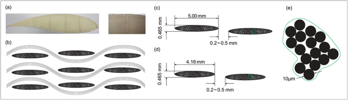
Geometry of the blade cross‐section; (a) root cross‐section shape; (b) woven geometry model of surface shell; (c) weft‐direction fiber bundles; (d) warp‐direction fiber bundles; and (e) fiber diameter

Another prominent feature of the blade is shown in Figure 2a,b. This pertains to the four vertically placed elements among the foam, attached to the lower and top surface laminates of the blade. These are referred to as the shear webs and extend from the fixation point at the root of blade up to almost the first third of the length of the blade. They are made out of the same composite material used for the outer shell, and their main function is to provide the blade with additional rigidity in the root region so as to avoid buckling problems.

2.2. Supporting frame

To represent the actual boundary conditions of the blade, in analogy to those applied on the Windspot 3.5 kW WT, a fix‐free set‐up was implemented during the dynamic testing. This was materialized with the aid of a steel frame, bolted on the ground via three concrete columns, whereon the blade is firmly clamped at one end through four bolts. To mitigate noise disturbance occurring from adjacent laboratory operations during the testing process, rubber absorbers were additionally placed between the specimen and the frame. A detailed layout of the experimental installation is depicted in Figure 3.

FIGURE 3.

The supporting steel frame: (a) top view, (b) front view, (c) bottom view, and (d) side view

2.3. Climate chamber

For the precise control of environmental conditions, the tests were conducted in a climate chamber where both temperature and humidity were controlled. Although humidity may, at high temperature conditions, have a considerable effect on air density ⁸⁵ and subsequently on global WT loads and energy production, herein it is not considered as an influential parameter for the structural properties of the experimental specimen. For the consistency though of the study, the relative humidity in the chamber was maintained constant, to a value of 60%, throughout the prosecution of the experiments. The blade was tested under varying temperature conditions, from −15°C to +40°C using a step of 5°C, with the aim of monitoring the temperature‐dependent material properties in both low ⁸⁶ and high ⁸⁷ regimes. A picture of the experimental installation in the climate chamber is shown in Figure 4a, including the climate controller, the shaker device, and the deployed measurement instruments.

FIGURE 4.

(a) Overview of the experimental set‐up in the climate chamber; (b) climate controller; (c) shaker with insulation foam box; (d) strain gauges s ₁ and s ₂ on low‐pressure side; (e) strain gauges s ₂₃ and s ₂₄ on high‐pressure side; (f) climate sensor; (g) cracks 1 and 2; and (h) crack 3

3. INSTRUMENTATION

3.1. Layout

A schematic representation of the deployed instrumentation is shown in Figure 5, where the entire arrangement consists of the input and output modules. The testing process initiates in Node 1 via creation of the excitation signal with the aid of a signal generator. The signal is transferred to the shaker device through a power amplifier and then imparted to the specimen via the small stringer. The ambient measurements along with the signals from the strain gauges are transmitted to the NI 9235 unit, part of the NI cDAQ‐9188 Data Acquisition (DAQ) system, and subsequently guided to Node 2. A slightly different path is followed for force and acceleration signals, since the former are first forwarded to an amplifier device and the latter are transmitted to a signal conditioner module. Both types of signals are then guided to the NI 9239 unit of the DAQ and finally rendered into retrievable data through Node 2, in conjunction with the stain and climate measurements.

FIGURE 5.

Workflow in data acquisition system

3.2. Humidity and temperature

Two humidity and temperature sensors have been installed on the downwind side of the specimen, as shown in Figure 6, in order to ensure that not only the ambient temperature but also the one on the blade surface has reached the target value. The sensitivity of humidity channels is 10 V/RH, which implies that Volt signals of humidity are transformed to relative humidity (RH) measurements according to $RH=10\ast H_{\mathrm{v}}$, where H _v is the humidity signal in Volts. On the other hand, the sensitivity of temperature sensors is 10 V/°C, while they are further characterized by an offset of 20°C. Therefore, the temperature signal T in degrees Celsius is obtained as follows: $T=10\ast T_{\mathrm{v}}-20$, where T _v is the measured temperature signal in Volts.

FIGURE 6.

Sensor configuration on the tested specimen (a) and on the specimen for temperature compensation (b)

3.3. Excitation

For the dynamic excitation of the specimen, a small electromechanical shaker device (Data Physics SignalForce V4) was utilized. The signals produced by the shaker were first transferred to the blade through a small stringer and then measured with a force sensor attached on the low‐pressure surface of the blade, as schematically shown in Figure 5. To ensure the smooth operation of the shaker along the entire temperature range of the experiments and to protect this against extreme conditions, the device was enclosed in an insulation box. An electrical bulb was also included in the box, to further assist in maintaining the specified operational regime of the shaker during low‐temperature tests.

Using this setting, two disparate types of excitation, both with duration of 120 s, were implemented for the dynamic testing of the blade, namely, (a) a white noise signal with effective frequency bandwidth between 0 and 400 Hz and (b) a sine sweep with frequencies ranging from 1 to 300 Hz. It should be noted that the frequency range of the latter was determined on the basis of a prototype finite element analysis, with the aim of stimulating at least the first six resonance frequencies ⁸⁸ of the structure.

3.4. Force sensor

Although the excitation is imparted to the blade via the shaker device and therefore it can be measured through the amplifier current output, it is not always the case that force and current are tracking together. For this reason, a force transducer (DYTRAN model 5860B, sensitivity 23.7 mV/N) has been deployed with the aim to keep track of the actual input signal sensed by the blade. This was mounted on the high‐pressure side of the specimen using a threaded adhesive base, at the exact location of the loading position, as shown in Figure 6.

3.5. Accelerometers

Accelerometers constitute a conventional and well‐established sensing technology in the context of SHM applications, appropriate for vibration‐based global damage detection methods. As such, a grid of eight accelerometers (PCB Piezotronics) with working range ±10 g and sensitivities reported in Table 2 was installed on the blade under consideration. These are indicated in Figure 6a by a _x , with x denoting the number of each specific sensor, and placed at fixed positions on the downwind side. These positions were determined upon analyzing the modal properties of the specimen using the reference finite element model.

TABLE 2.

Sensitivity of acceleration and force sensors

Channel	a 1	a 2	a 3	a 4	a 5	a 6	a 7	a 8	f 1
Sensitivity (mV/unit a )	51.4	51.7	51.8	52.0	52.2	52.6	51.4	52.6	23.7

^a Unit is m/s ² for accelerometers and N for the force sensor.

3.6. Strain gauges

Likewise, strain measurements are widely used for damage detection ⁸⁹ , ⁹⁰ and localization ⁹¹ on structural and mechanical systems, with numerous applications on WT blades. ⁹² Herein, a network of 18 strain gauges is deployed, comprising two types of devices: unidirectional strain gauges (HBM 1‐LY48‐20/120) and rosettes (HBM 1‐RY88‐6/120) with three measuring grids arranged at an angle of 0°/45°/90°. The strain gauges were attached on the structure using two different configurations, as schematically shown in Figure 6a. Their locations were determined again through a prototype finite element modal analysis, with the aim of rendering observable all vibration modes, in the frequency range of interest [0–200 Hz]. A set of common measurement grids denoted by s _x , with subscript x indicating the number of channel, was utilized for both configurations, while an additional set of configuration‐specific strain grids denoted by $s_x^{(y)}$, with superscript y indicating the number of set‐up, was employed. The difference between the two layouts consists in the orientation of the deployed unidirectional gauges; namely, the first layout corresponds to the unidirectional gauges aligned with the z‐axis, while the second one aims at monitoring the strain along the y direction and therefore gauges are brought into alignment with y‐axis. It should be noted that channels s ₁ and s ₂ on the low‐pressure side as well as channels s ₂₃ and s ₂₄ on the upwind side were kept aligned with Z‐axis in both configurations so as to enable the estimation of bending moment at the root of the blade.

Due to the execution of experiments under varying environmental conditions, strain measurements need to be corrected in order to account for the effect of temperature. The latter is not only dependent on the thermal properties of the test specimen but additionally on the characteristics of the strain gauges as such. Since two different types of gauges were employed in the present study, the sensitivity of each type on temperature variability was separately tested on the unloaded specimen, with the two devices demonstrating identical response. As a result, temperature corrections on strain measurements were based on the register of a single uniaxial strain gauge, that is, sensor s ₁₆ , attached on a duplicate of the specimen, as shown in Figure 6b, and subjected to the same environmental variations.

4. DAMAGE SCENARIOS AND EXPERIMENTAL PROCEDURE

4.1. Damage scenarios

Apart from the initially healthy state, two distinct families of damages of varying severity are studied in the same range of temperature conditions. It should be underlined at this point that damage is not considered as an exclusively degrading or destructive effect but may encompass any change introduced into a system that can affect the structural performance thereof. Within this context, the first group of damage scenarios attempts to simulate icing accretion, which constitutes a rather typical phenomenon in structures located at cold climate areas and may affect various aspects of a WT system when occurring on blades. ⁹³ Icing primarily affects aerodynamic performance, which is significantly disturbed by the increased roughness on the blade surface and leads to either reduced power production or overloading on stall‐regulated WTs. Moreover, all turbine components are exposed to increased loads, induced by the additional ice mass, while the lifetime of the structure may be significantly shortened due to the imbalance between blades. Although icing is characterized as a distributed phenomenon, herein it is represented by adhering a set of lumped masses on specific locations, as shown in Figure 6a. Such a representation is not intended to reproduce the real mechanism as such but to merely provide a basis for testing the various SHM methods on damage detection, localization, and quantification.

The second group of damage scenarios focuses on the investigation of cracks of varying characteristics, that is, length and location, which are physically introduced on the structure as surface cuts. The location of these cracks was determined on the basis of existing experimental ⁹⁴ and simulation‐based ⁹⁵ contributions concerning damage on WT blades, reporting positions where flaws are most likely to occur. ⁹⁶ , ⁹⁷ Based on the findings of these established works, three different locations were selected at 17%, 30%, and 50% of the blade's longitudinal axis, as depicted in Figure 6a, with the effect of each crack investigated for lengths of 5, 10, and 15 cm, all with the same depth and width of 4 and 1.5 mm, respectively. This results in a combination of nine cracked scenarios, which are documented in Table 3 along with the first group.

TABLE 3.

List of experimental cases and number of tests conducted for each case

Case label	Description			Number of experiments
R	Healthy state			21 per temperature per set‐up
A	Added mass 1 × 44 g			6 per temperature per set‐up
B	Added mass 2 × 44 g			6 per temperature per set‐up
C	Added mass 3 × 44 g			6 per temperature per set‐up
D	Crack 1: l 1  = 5 cm			6 per temperature per set‐up
E	Crack 1: l 1  = 5 cm,	Crack 2: l 2  = 5 cm		6 per temperature per set‐up
F	Crack 1: l 1  = 5 cm,	Crack 2: l 2  = 5 cm,	Crack 3: l 3  = 5 cm	6 per temperature per set‐up
G	Crack 1: l 1  = 10 cm,	Crack 2: l 2  = 5 cm,	Crack 3: l 3  = 5 cm	6 per temperature per set‐up
H	Crack 1: l 1  = 10 cm,	Crack 2: l 2  = 10 cm,	Crack 3: l 3  = 5 cm	6 per temperature per set‐up
I	Crack 1: l 1  = 10 cm,	Crack 2: l 2  = 10 cm,	Crack 3: l 3  = 10 cm	6 per temperature per set‐up
J	Crack 1: l 1  = 15 cm,	Crack 2: l 2  = 10 cm,	Crack 3: l 3  = 10 cm	6 per temperature per set‐up
K	Crack 1: l 1  = 15 cm,	Crack 2: l 2  = 15 cm,	Crack 3: l 3  = 10 cm	6 per temperature per set‐up
L	Crack 1: l 1  = 15 cm,	Crack 2: l 2  = 15 cm,	Crack 3: l 3  = 15 cm	6 per temperature per set‐up

4.2. Test process

The experimental cases reported in Table 3 are tested for all combinations of excitations, temperature conditions, and sensor configurations. Initially, the healthy specimen is mounted on the steel frame, and the temperature in the climate chamber is adjusted at the minimum value of interest, that is, −15°C, until the temperature sensors attached on the blade reach the specified value. With the strain sensors arranged according to the first configuration, the blade is first tested using a sine sweep excitation, and subsequently, a set of 20 tests is conducted using white noise input. The strain gauges are then switched to the second configuration, and the blade is tested again using a sine sweep and 20 white noise input signals. The same workflow is then followed for all temperature values of the healthy structure. The process is finally repeated for all damaged scenarios, with the difference that only 5 instead of 20 tests are carried out using white noise excitation.

For the sake of brevity, each experimental case is referred to as X _y with label X denoting the model state as defined in Table 3, that is, Healthy, Damage A, Damage B, and so forth, and subscript y indicating the testing temperature. With the exception of the healthy state, which is assigned as the basis of reference and labeled with R, each damaged scenario is marked using a letter notation from A to L, according to the notation documented in Table 3. Therefore, the abbreviation R ₋₁₅ is henceforth adopted when referring to the healthy case tested in −15°C and similarly, L ₊₄₀ insinuates the test performed in 40°C for the model noted as Damage L in Table 3.

5. DATA PROFILE

The entire data set produced from the experiments is publicly available through Zenodo, and in what follows, a set of indicative measurement signals is graphically represented in both time and frequency domain. To provide a holistic view of the study and available data, the selected signals do not only pertain to response measurements, that is, strains and accelerations, but also to excitation signals and ambient indices. In order to further afford an insightful picture of the investigated damage scenarios, the signals to be presented are acquired from the three extremities of the experimental spectrum, that is, the nominal state R, the test with three added masses C, and the most excessively cracked case L. Moreover, the variation of system dynamic properties across all temperature points and damage scenarios is presented in terms of the identified frequencies, mode shapes, and mode shape curvatures.

5.1. Data in time domain

The time histories of temperature and relative humidity in the climate chamber during execution of test R ₊₃₀ are shown in Figure 7a–d, so as to highlight the actual ambient conditions sensed by the blade. Figure 7e–h depicts the sine sweep excitation imparted to the specimen during test case R ₋₁₅ , in conjunction with the white noise input utilized for experiment R ₊₄₀ . The acceleration measurements obtained from these tests are shown in Figure 8a,b and c,d for channels a ₁ and a ₈ , respectively. Accordingly, Figure 8e,f and g,h present the strain response measured at channels s ₁ and s ₂₁ when cases R ₋₁₅ and R ₊₄₀ are tested with the input signals of Figure 7e,f and g,h, respectively.

FIGURE 7.

Time history of temperature (orange), humidity (green), and input force (blue) measurements; (a, b) temperature for test case R ₊₃₀ ; (c, d) humidity for test case R ₊₃₀ ; (e, f) sine sweep excitation for test case R ₋₁₅ ; and (g, h) white noise excitation for test case R ₊₄₀

FIGURE 8.

Time history of acceleration (red) and strain (yellow) measurements; (a, b) channel a ₁ for test case R ₋₁₅ excited by sine sweep; (c, d) channel a ₈ for test case R ₊₄₀ excited by white noise; (e, f) channel s ₁ for test case R ₋₁₅ excited by sine sweep; and (g, h) channel s ₂₁ for test case R ₊₄₀ excited by white noise

5.2. Data in frequency domain

The response measurements of some representative channels are visualized in the frequency domain as well, through their respective power spectral density (PSD) plots. In so doing, the measured signals were first sampled at 833 Hz, upon down‐sampling from 1666 Hz, and thereafter low‐pass filtered with a cut‐off frequency of 380 Hz, to yield a signal of 10,000 samples, which corresponds to a duration of 12 s.

Figure 9a,b illustrates the PSD of channels a ₃ and a ₈ , respectively, (Figure 6) obtained from the experimental cases R ₊₂₅ , C ₊₂₅ , and L ₊₂₅ using white noise excitation. The PSD is calculated using the Welch's segment averaging estimator with Hanning window applied in segments of 16,384 samples. Accordingly, Figure 9c,d shows the PSD of channels s ₉ and s ₁₄ , respectively, using the same settings of Welch's estimator, with measurements from experimental cases R ₊₂₅ , C ₊₂₅ , and L ₊₂₅ stimulated by sine sweep input. The regions of the peaks corresponding to the flapwise and torsional modes for all three cases R ₊₂₅ , C ₊₂₅ , and L ₊₂₅ are highlighted in Figure 9 by the gray zones, with the first three containing the flapwise modes and the last two representing the first and second torsional modes. Based on the width of each region, it can be observed that the effect of cracks is more pronounced on the torsional modes than on the bending modes in flapwise direction.

FIGURE 9.

Power spectral density of channels a ₃ (a), a ₈ (b), s ₉ (c), and s ₁₄ (d) from cases R ₊₂₅ , C ₊₂₅ , and L ₊₂₅ tested with sine sweep excitation

5.3. Dynamic properties

The experimental tests are in this section presented by means of the identified dynamic properties across the examined environmental spectrum and damage conditions. It should be noted that due to the curved geometry of the blade surface, the measurement axis of acceleration sensors is not well aligned with the x‐axis of the coordinate system defined in Figure 6. As such, not only flapwise and torsional modes are observable with the adopted set‐up but also the ones in edgewise direction. This can be verified by the PSD plots of acceleration channels a ₃ and a ₈ , as depicted in Figure 9, in which the first edgewise modes are slightly distinguishable between the first and second flapwise modes, at around 14 and 50 Hz, respectively. Due to this faint contribution, which is owed to the small projection of edgewise vibration response on the measurement direction, edgewise modes cannot be accurately identified using only accelerations.

5.3.1. Natural frequencies and vibration modes

The natural frequencies and vibration modes are identified using the covariance‐based stochastic subspace identification (SSI‐Cov), for which acceleration signals a ₁ , a ₂ , a ₃ , a ₅ , a ₆ , a ₇ , and a ₈ are utilized. The variability of the first three natural frequencies with respect to temperature is illustrated in the left‐hand column of Figure 10, where an almost linear dependency law is observed. In order to offer the possibility of dealing with nonlinear environmental effects, which are often encountered in such composite structures, ⁸⁷ the reader is referred to the numerical companion paper which assumes an exponential dependency of the material properties on temperature. It should be also noted that the corresponding modes of the frequencies reported in Figure 10, which represent bending behavior in flapwise direction, remain unaffected from temperature variations. This is owed to the fact that the specimen is subjected to a uniform temperature field while the inner foam, which could trigger such changes due to the different temperature‐dependency law, has negligible structural contribution.

FIGURE 10.

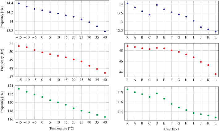
Variation of the first three flapwise natural frequencies; left column depicts the effect of temperature to the reference case (R); right column depicts the influence of damage at 25°C temperature

Accordingly, the right‐hand column of Figure 10 depicts the values of the first three natural frequencies with respect to the damage scenarios, which are extracted from tests at 25°C. It can be seen that the attachment of additional mass on the blade has a consistent effect on the reduction of natural frequencies, which is owed to the fact that both the position and amount of mass are well controlled. On the other hand, the introduction of cracks is practically impossible to control in laboratory conditions, creating thus a non‐regular trend as evidenced by the variation between cases D and L. This non‐quantifiable effect is addressed in the numerical counterpart of this paper, where the amount and location of damage are rigorously defined on a finite element (FE) model of the specimen. The effect of damage on the modes is presented in Figure 11, which depicts the first three flapwise modes as identified by acceleration sensors a ₁ , a ₃ , a ₅ , and a ₇ .

FIGURE 11.

Variation of the first (a), second (b), and third (c) vibration mode with respect to damage scenarios involving cracks

5.3.2. Mode shape curvature

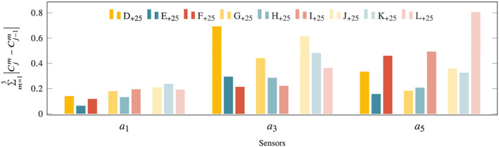
Although the frequencies and mode shapes undergo noticeable changes due to the introduced cracks, the localization of damage is not possible using only these features. As such, the use of mode shape curvature for damage localization is further demonstrated, since it is reported to be one of the most sensitive modal‐based indicators. ⁹⁸ , ⁹⁹ The calculation of such feature is straightforward as soon as the vibration modes are identified, and it should be further noted that a collinear configuration of the measurement points is required in order to preserve its physical interpretability. Indicatively, the mode shape curvature is calculated for all three flapwise modes of models R, D, E, F, G, H, I, J, K, L at temperature 25°C, and an indication of damage location is obtained as the sum of absolute difference between the mode shape curvatures of two different system states. For instance, if ${\mathrm{C}}_{{\mathrm{D}}_{+25}}^m$ and ${\mathrm{C}}_{{\mathrm{R}}_{+25}}^m$ denote the mth mode curvature of test cases D ₊₂₅ and R ₊₂₅ , respectively, an indication of the damage location is obtained by summing all terms $\left|{\mathrm{C}}_{{\mathrm{D}}_{+25}}^m-{\mathrm{C}}_{{\mathrm{R}}_{+25}}^m\right|$ for $m=1,\dots ,n_{\mathrm{m}}$, where n _m is the number of identified modes.

In order for the measurement points to be collinear, the vibration modes are initially identified using accelerometers a ₁ , a ₃ , a ₅ , and a ₇ , and the curvature is subsequently computed at a ₁ , a ₃ , and a ₅ . The successive change of curvature from test case R ₊₂₅ to L ₊₂₅ , excluding test cases A, B, and C, is illustrated in Figure 12, where x‐axis refers to the measurement points a ₁ , a ₃ , and a ₅ , while y‐axis represents the change of curvature between each test and its previous one. Therefore, the red bar at a ₁ corresponds to the curvature change between cases F ₊₂₅ and E ₊₂₅ at the location of accelerometer a ₁ , while the yellow bars represent the curvature changes between states D ₊₂₅ and R ₊₂₅ . It is seen that all three locations of cracks are more noticeably traced at a ₃ and a ₅ than at a ₁ , which is owed to the fact that the latter is always between the cracked region and the support. Moreover, it can be consistently observed that the cracks introduced between sensors a ₁ and a ₃ , either at 0.17 or at 0.30 L, have a more pronounced signature on the curvature change at a ₃ , while the cracks at 0.5 L are mainly reflected by the curvature changes at a ₅ .

FIGURE 12.

Sum of the absolute change of mode shape curvature using the first three flapwise vibration modes for the test cases involving cracks (D–L) at 25°C temperature

6. CONCLUSIONS

The operational and environmental variations on WT structures comprise one of the main challenges for deploying SHM methodologies on in‐service blades. Besides the varying boundary conditions and the exposure to non‐uniform thermal gradients, ¹⁰⁰ it is reported that fluctuations in ambient temperatures exert a strong impact on the vibration features of WT blades ¹⁰¹ and therefore damage‐induced structural changes may often be masked by changes due to ambient temperature effects. With numerous WTs operating in harsh and highly varying climate conditions, it is thus imperative that temperature effects be further and more exhaustively investigated so that their influences are eliminated.

This contribution constitutes a benchmark study on a small‐scale WT blade, with the aim of establishing a common baseline for performance assessment, verification, and validation of the broad‐spectrum methodologies on the realm of SHM. A main challenge in the design of these tests lies in experimentally producing the desired system conditions, which are intended to represent the actual SHM challenges. Here, we focus on the aspect of environmental variability by conducting a series of tests under pristine and damaged conditions on the small‐scale blade within a climatic chamber. Although conducted on a WT blade, the study deals with issues of universal interest in the SHM community:

• effect of environmental conditions, that is, temperature, on vibration features;

• investigation of typical damage scenarios with varying degree of severity and multiple locations; and

• implementation of mixed sensor grids, including accelerometers, strain gauges, and temperature sensors;

and may well serve as a breeding ground for the investigation of techniques intended not only for damage detection, localization, and quantification but also for modal identification algorithms, model updating approaches, and optimal sensor placement schemes. The vibration data from the conducted experiments are made available at Zenodo.

Ou Y, Tatsis KE, Dertimanis VK, Spiridonakos MD, Chatzi EN. Vibration‐based monitoring of a small‐scale wind turbine blade under varying climate conditions. Part I: An experimental benchmark. Struct Control Health Monit. 2021;28:e2660. 10.1002/stc.2660

REFERENCES

- 1. Vandiver JK. Detection of structural failure on fixed platforms by measurement of dynamic response. In: Proceedings of the 7th Offshore Technology Conference. Houston, USA; 1975:243‐252. [Google Scholar]
- 2. Kenley RM, Dodds CJ. West Sole WE Platform: detection of damage by structural response measurements. In: Proceedings of the 12th Offshore Technology Conference. Houston, USA; 1980:111‐118. [Google Scholar]
- 3. James G, Mayes R, Carne T, Garth R. Damage detection and health monitoring of operational structures. SAND‐94‐1181C; CONF‐941142‐22, Albuquerque NM, Sandia National Laboratories; 1994. [Google Scholar]
- 4. James G. Development of structural health monitoring techniques using dynamics testing. SAND‐96‐0810, Albuquerque NM, Sandia National Laboratories; 1996. [Google Scholar]
- 5. Doebling SW, Farrar CR, Prime MB, Shevitz DW. Damage identification and health monitoring of structural and mechanical systems from changes in their vibration characteristics: a literature review. LA‐13070‐MS, Los Alamos NM: Los Alamos National Laboratory; 1996. [Google Scholar]
- 6. Doebling SW, Farrar CR, Prime MB. A summary review of vibration‐based damage identification methods. Shock Vib. 1998;30(2):91‐105. 10.1177/058310249803000201 [DOI] [Google Scholar]
- 7. Sohn H, Farrar CR, Hemez FM, et al. A review of structural health monitoring literature. tech. rep. LA‐13976‐MS, Los Alamos, NM: Los Alamos National Laboratory; 2004. [Google Scholar]
- 8. Farrar CR, Worden K. An introduction to structural health monitoring. Philos Trans Royal Soc A. 2007;365:303‐315. 10.1098/rsta.2006.1928 [DOI] [PubMed] [Google Scholar]
- 9. Sohn H. Effects of environmental and operational variability on structural health monitoring. Philos Trans Royal Soc A Math Phys Eng Sci. 2007;365(1851):539‐560. 10.1098/rsta.2006.1935 [DOI] [PubMed] [Google Scholar]
- 10. Worden K, Farrar CR, Jonathan H, Michael T. A review of nonlinear dynamics applications to structural health monitoring. Struct Control Health Monitor. 2008;15:540‐567. 10.1002/stc [DOI] [Google Scholar]
- 11. Deraemaeker A, Worden K. New Trends in Vibration Based Structural Health Monitoring. Vol 39. Udine: Springer; 2008. [Google Scholar]
- 12. Tcherniak D, Chauhan S, Hansen MH. Applicability limits of operational modal analysis to operational wind turbines. In: Conference Proceedings of the Society for Experimental Mechanics Series. Jacksonville, Florida USA; 2010:317‐327. [Google Scholar]
- 13. Ozbek M, Meng F, Rixen DJ. Challenges in testing and monitoring the in‐operation vibration characteristics of wind turbines. Mech Syst Signal Process. 2013;41(1‐2):649‐666. 10.1016/j.ymssp.2013.07.023 [DOI] [Google Scholar]
- 14. Yang W, Tavner PJ, Crabtree CJ, Feng Y, Qiu Y. Wind turbine condition monitoring: technical and commercial challenges. Wind Energy. 2014;17:673‐693. 10.1002/we [DOI] [Google Scholar]
- 15. Hameed Z, Hong YS, Cho YM, Ahn SH, Song CK. Condition monitoring and fault detection of wind turbines and related algorithms: a review. Renew Sustain Energy Rev. 2009;13(1):1‐39. 10.1016/j.rser.2007.05.008 [DOI] [Google Scholar]
- 16. Wymore ML, Van Dam JE, Ceylan H, Qiao D. A survey of health monitoring systems for wind turbines. Renew Sustain Energy Rev. 2015;52(1069283):976‐990. 10.1016/j.rser.2015.07.110 [DOI] [Google Scholar]
- 17. Antoniadou I, Dervilis N, Papatheou E, Maguire AE, Worden K. Aspects of structural health and condition monitoring of offshore wind turbines. Philos Trans Royal Soc A Math Phys Eng Sci. 2015;373(2035):20140075‐20140075. 10.1098/rsta.2014.0075 [DOI] [PMC free article] [PubMed] [Google Scholar]
- 18. Hu WH, Thöns S, Rohrmann RG, Said S, Rücker W. Vibration‐based structural health monitoring of a wind turbine system Part II: environmental/operational effects on dynamic properties. Eng Struct. 2015;89:273‐290. 10.1016/j.engstruct.2014.12.035 [DOI] [Google Scholar]
- 19. Hu WH, Thöns S, Rohrmann RG, Said S, Rücker W. Vibration‐based structural health monitoring of a wind turbine system. Part I: resonance phenomenon. Eng Struct. 2015;89:260‐272. 10.1016/j.engstruct.2014.12.034 [DOI] [Google Scholar]
- 20. Carne TG, James GH. The inception of OMA in the development of modal testing technology for wind turbines. Mech Syst Sig Process. 2010;24(5):1213‐1226. 10.1016/j.ymssp.2010.03.006 [DOI] [Google Scholar]
- 21. Devriendt C, Magalhães F, Weijtjens W, De Sitter G, Cunha Á, Guillaume P. Structural health monitoring of offshore wind turbines using automated operational modal analysis. Struct Health Monitor. 2014;13(6):644‐659. 10.1177/1475921714556568 [DOI] [Google Scholar]
- 22. Martinez‐Luengo M, Kolios A, Wang L. Structural health monitoring of offshore wind turbines: a review through the Statistical Pattern Recognition Paradigm. Renew Sustain Energy Rev. 2016;64:91‐105. 10.1016/j.rser.2016.05.085 [DOI] [Google Scholar]
- 23. Bogoevska S, Spiridonakos M, Chatzi E, Dumova‐Jovanoska E, Höffer R. A data‐driven diagnostic framework for wind turbine structures: a holistic approach. Sensors (Switzerland). 2017;17(4):720. 10.3390/s17040720 [DOI] [PMC free article] [PubMed] [Google Scholar]
- 24. Avendaño‐Valencia LD, Chatzi EN, Koo KY, Brownjohn JMW. Gaussian process time‐series models for structures under operational variability. Front Built Environ. 2017;3:1‐19. 10.3389/fbuil.2017.00069 [DOI] [Google Scholar]
- 25. Avendaño‐Valencia LD, Fassois SD. Damage/fault diagnosis in an operating wind turbine under uncertainty via a vibration response Gaussian mixture random coefficient model based framework. Mech Systems Sig Process. 2017;91:326‐353. 10.1016/j.ymssp.2016.11.028 [DOI] [Google Scholar]
- 26. Dervilis N, Choi M, Taylor SG, et al. On damage diagnosis for a wind turbine blade using pattern recognition. J Sound Vib. 2014;333(6):1833‐1850. 10.1016/j.jsv.2013.11.015 [DOI] [Google Scholar]
- 27. Dao PB, Staszewski WJ, Barszcz T, Uhl T. Condition monitoring and fault detection in wind turbines based on cointegration analysis of SCADA data. Renew Energy. 2018;116:107‐122. 10.1016/j.renene.2017.06.089 [DOI] [Google Scholar]
- 28. Moradi M, Sivoththaman S. MEMS multisensor intelligent damage detection for wind turbines. IEEE Sens J. 2015;15(3):1437‐1444. 10.1109/JSEN.2014.2362411 [DOI] [Google Scholar]
- 29. Cairns DS, Palmer N, Ehresman J. Embedded sensors for composite wind turbine blades. In: AIAA/ASME/ASCE/AHS/ASC Structures: Structural Dynamics and Materials Conference. Orlando, Florida USA; 2010. [Google Scholar]
- 30. Song G, Li H, Gajic B, Zhou W, Chen P, Gu H. Wind turbine blade health monitoring with piezoceramic‐based wireless sensor network. Int J Smart Nano Mater. 2013;4(3):150‐166. 10.1080/19475411.2013.836577 [DOI] [Google Scholar]
- 31. Kim S, Adams DE, Sohn H, et al. Crack detection technique for operating wind turbine blades using Vibro‐Acoustic Modulation. Struct Health Monitor. 2014;13(6):660‐670. 10.1177/1475921714553732 [DOI] [Google Scholar]
- 32. LeBlanc B, Niezrecki C, Avitabile P, Chen J, Sherwood J. Damage detection and full surface characterization of a wind turbine blade using three‐dimensional digital image correlation. Struct Health Monitor. 2013;12(5‐6):430‐439. 10.1177/1475921713506766 [DOI] [Google Scholar]
- 33. Currie M, Saafi M, Tachtatzis C, Quail F. Structural integrity monitoring of onshore wind turbine concrete foundations. Renew Energy. 2015;83:1131‐1138. 10.1016/j.renene.2015.05.006 [DOI] [Google Scholar]
- 34. Bai X, He M, Ma R, Huang D. Structural condition monitoring of wind turbine foundations. Energy. 2017;170:116‐134. 10.1680/jener.16.00012 [DOI] [Google Scholar]
- 35. Perry M, Fusiek G, Niewczas P, Rubert T, McAlorum J. Wireless concrete strength monitoring of wind turbine foundations. Sensors (Switzerland). 2017;17(12):1‐22. 10.3390/s17122928 [DOI] [PMC free article] [PubMed] [Google Scholar]
- 36. Rubert T, Id MP, Fusiek G, et al. Field demonstration of real‐time wind turbine foundation strain monitoring. Sensors (Switzerland). 2018;18(1):1‐23. 10.3390/s18010097 [DOI] [PMC free article] [PubMed] [Google Scholar]
- 37. Weihnacht B, Frankenstein B, Gaul T, Neubeck R, Schubert L. Monitoring of welded seams on the foundations of offshore wind turbines. Insight Non‐Destruct Testing Cond Monitor. 2017;59(2):72‐76. 10.1784/insi.2017.59.2.72 [DOI] [Google Scholar]
- 38. Weijtjens W, Verbelen T, Sitter GD, Devriendt C. Foundation structural health monitoring of an offshore wind turbine—a full‐scale case study. Struct Health Monitor. 2016;15(4):389‐402. 10.1177/1475921715586624 [DOI] [Google Scholar]
- 39. Weijtens W, Noppe N, Verbelen T, Iliopoulos A, Devriendt C. Offshore wind turbine foundation monitoring, extrapolating fatigue measurements from fleet leaders to the entire wind farm. J Phys Conf Ser. 2016;753(9):092018. 10.1088/1742-6596/753/9/092018 [DOI] [Google Scholar]
- 40. Iliopoulos A, Weijtjens W, Van Hemelrijck D, Devriendt C. Fatigue assessment of offshore wind turbines on monopile foundations using mulit‐band modal expansion. Wind Energy. 2017;20:1463‐1479. 10.1002/we [DOI] [Google Scholar]
- 41. Mylonas C, Abdallah I, Chatzi EN. Deep unsupervised learning for condition monitoring and prediction of high dimensional data with application on windfarm SCADA data. In: Proceedings of the 37th IMAC Conference and Exposition on Structural Dynamics: Predictive Modeling for Engineering Design and Decision Making (IMAC XXXVII 2019). Orlando, Florida USA; 2019:189. [Google Scholar]
- 42. Avendaño‐Valencia LD, Fassois SD. Stationary and non‐stationary random vibration modelling and analysis for an operating wind turbine. Mech Syst Sig Process. 2014;47:263‐285. [Google Scholar]
- 43. Van der Male P, Lourens E. Operational vibration‐based response estimation for offshore wind lattice structures. In: Conference Proceedings of the Society for Experimental Mechanics Series. Cham; 2015:83‐96. [Google Scholar]
- 44. Gillijns S, De Moor B. Unbiased minimum‐variance input and state estimation for linear discrete‐time systems with direct feedthrough. Automatica. 2007;43(5):934‐937. 10.1016/j.automatica.2006.11.016 [DOI] [Google Scholar]
- 45. Jonkman BJ. TurbSim User's Guide. NREL/TP‐500‐46198. Battelle, CO, USA: NREL; 2009. [Google Scholar]
- 46. Tatsis K, Lourens E. A comparison of two Kalman‐type filters for robust extrapolation of offshore wind turbine support structure response. In: Proceedings of the Fifth International Symposium on Life‐Cycle Civil Engineering (IALCCE 2016). Delft, The Netherlands; 2016:209‐216. [Google Scholar]
- 47. Maes K, Iliopoulos A, Weijtjens W, Devriendt C, Lombaert G. Dynamic strain estimation for fatigue assessment of an offshore monopile wind turbine using filtering and modal expansion algorithms. Mech Syst Sign Process. 2016;76‐77:592‐611. 10.1016/j.ymssp.2016.01.004 [DOI] [Google Scholar]
- 48. Tatsis K, Dertimanis V, Abdallah I, Chatzi E. A substructure approach for fatigue assessment on wind turbine support structures using output‐only measurements. Proced Eng. 2017;199:1044‐1049. 10.1016/j.proeng.2017.09.285 [DOI] [Google Scholar]
- 49. Tatsis K, Chatzi E, Lourens EM. Reliability prediction of fatigue damage accumulation on wind turbines support structures. In: Proceedings of the 2nd International Conference on Uncertainty Quantification in Computational Sciences and Engineering. Rhodes Island, Greece; 2017:76‐89. [Google Scholar]
- 50. Oliveira G, Magalhães F, Cunha Á, Caetano E. Continuous dynamic monitoring of an onshore wind turbine. Eng Struct. 2018;164:22‐39. 10.1016/j.engstruct.2018.02.030 [DOI] [Google Scholar]
- 51. Zuo H, Bi K, Hao H. Dynamic analyses of operating offshore wind turbines including soil‐structure interaction. Eng Struct. 2018;157:42‐62. 10.1016/j.engstruct.2017.12.001 [DOI] [Google Scholar]
- 52. Lindsay G, Connor R, Crosthwaite S, et al. Summary of wind turbine accident data to 31 December 2016. tech. rep., Caithness Windfarm Information Forum; 2016.
- 53. Ghoshal A, Sundaresan MJ, Schulz MJ, Frank Pai P. Structural health monitoring techniques for wind turbine blades. J Wind Eng Ind Aerodyn. 2000;85(3):309‐324. 10.1016/S0167-6105(99)00132-4 [DOI] [Google Scholar]
- 54. Sørensen BF, Lading L, Sendrup P, et al. Fundamentals for remote structural health monitoring of wind turbine blades—a preproject. tech. rep. No. 1336. Roskilde: Risø National Laboratory; 2002. [Google Scholar]
- 55. Tsai CS, Hsieh CT, Huang SJ. Enhancement of damage‐detection of wind turbine blades via CWT‐based approaches. IEEE Trans Energy Conv. 2006;21(3):776‐781. 10.1109/TEC.2006.875436 [DOI] [Google Scholar]
- 56. Dervilis N, Choi M, Antoniadou I, et al. Novelty detection applied to vibration data from a CX‐100 wind turbine blade under fatigue loading. J Phys Conf Ser. 2012;382(1):012047. 10.1088/1742-6596/382/1/012047 [DOI] [Google Scholar]
- 57. Pang YR, Lv ZH, Liang XM, et al. Acoustic emission attenuation and source location of resin matrix for wind turbine blade composites. Adv Mater Res. 2014;912‐914:36‐39. 10.4028/www.scientific.net/amr.912-914.36 [DOI] [Google Scholar]
- 58. Bouzid OM, Tian GY, Cumanan K, Moore D. Structural health monitoring of wind turbine blades: acoustic source localization using wireless sensor networks. J Sens. 2015;2015. 10.1155/2007/73624 [DOI] [Google Scholar]
- 59. Tang J, Soua S, Mares C, Gan TH. An experimental study of acoustic emission methodology for in service condition monitoring of wind turbine blades. Renew Energy. 2016;99:170‐179. 10.1016/j.renene.2016.06.048 [DOI] [Google Scholar]
- 60. Muñoz CQG, Márquez FPG. A new fault location approach for acoustic emission techniques in wind turbines. Energies. 2016;9(1):40. 10.3390/en9010040 [DOI] [Google Scholar]
- 61. Bo Z, Yanan Z, Changzheng C. Acoustic emission detection of fatigue cracks in wind turbine blades based on blind deconvolution separation. Fatigue Fract Eng Mater Struct. 2017;40(6):959‐970. 10.1111/ffe.12556 [DOI] [Google Scholar]
- 62. Yang B, Sun D. Testing, inspecting and monitoring technologies for wind turbine blades: a survey. Renew Sustain Energy Rev. 2013;22:515‐526. 10.1016/j.rser.2012.12.056 [DOI] [Google Scholar]
- 63. Yang W, Peng Z, Wei K, Tian W. Structural health monitoring of composite wind turbine blades: challenges, issues and potential solutions. IET Renew Power Gener. 2017;11(4):411‐416. 10.1049/iet-rpg.2016.0087 [DOI] [Google Scholar]
- 64. Larsen G, Berring P, Tcherniak D, Nielsen P, Branner K. Effect of a damage to modal parameters of a wind turbine blade. In: Proceedings of the 7th European Workshop on Structural Health Monitoring EWSHM. Nantes, France; 2014:261‐269. [Google Scholar]
- 65. Lorenzo ED, Petrone G, Manzato S, Peeters B, Desmet W, Marulo F. Damage detection in wind turbine blades by using operational modal analysis. Struct Health Monitor. 2016;15(3):289‐301. 10.1177/1475921716642748 [DOI] [Google Scholar]
- 66. Ou Y, Chatzi EN, Dertimanis VK, Spiridonakos MD. Vibration‐based experimental damage detection of a small‐scale wind turbine blade. Struct Health Monitor. 2017;16(1):79‐96. 10.1177/1475921716663876 [DOI] [PMC free article] [PubMed] [Google Scholar]
- 67. Ou Y, Dertimanis VK, Chatzi EN. Experimental damage detection of a wind turbine blade under varying operational conditions. In: Proceedings of the International Conference on Noise and Vibration Engineering 2016 (ISMA 2016) and International Conference on Uncertainty in Structural Dynamics (USD 2016). Leuven, Belgium; 2016:4183‐4198. [Google Scholar]
- 68. Islam MR, Guo Y, Zhu J. A review of offshore wind turbine nacelle: technical challenges, and research and developmental trends. Renew Sustain Energy Rev. 2014;33:161‐176. 10.1016/j.rser.2014.01.085 [DOI] [Google Scholar]
- 69. Shin D, Kim H, Ko K. Analysis of wind turbine degradation via the nacelle transfer function. J Mech Sci Technol. 2015;29(9):4003‐4010. 10.1007/s12206-015-0846-y [DOI] [Google Scholar]
- 70. Helsen J, Devriendt C, Weijtjens W, Guillaume P. Experimental dynamic identification of modeshape driving wind turbine grid loss event on nacelle testrig. Renew Energy. 2016;85:259‐272. 10.1016/j.renene.2015.06.046 [DOI] [Google Scholar]
- 71. Feng Y, Qiu Y, Crabtree CJ, Long H, Tavner PJ. Monitoring wind turbine gearboxes. Wind Energy. 2013;16:728‐740. 10.1002/we [DOI] [Google Scholar]
- 72. Astolfi D, Scappaticci L, Terzi L. Fault diagnosis of wind turbine gearboxes through temperature and vibration data. Int J Renew Energy. 2017;7(2):965‐976. [Google Scholar]
- 73. Liu J, Shao Y. Dynamic modeling for rigid rotor bearing systems with a localized defect considering additional deformations at the sharp edges. J Sound Vib. 2017;398:84‐102. 10.1016/j.jsv.2017.03.007 [DOI] [Google Scholar]
- 74. Farrar CR, Baker WE, Bell TM, et al. Dynamic characterization and damage detection in the I‐40 bridge over the Rio Grande. LA‐12767‐MS, Los Alamos, NM: Los Alamos National Laboratory; 1994. [Google Scholar]
- 75. Maeck J, De Roeck G. Description of Z24 benchmark. Mech Systems Signal Process. 2003;17(1):127‐131. 10.1006/mssp.2002.1548 [DOI] [Google Scholar]
- 76. Molina FJ, Pascual R, Golinval JC. Description of the steelquake benchmark. Mech Syst Signal Process. 2003;17(1):77‐82. 10.1006/mssp.2002.1542 [DOI] [Google Scholar]
- 77. Li S, Li H, Lan C, Zhou W, Ou J.. SMC structural health monitoring benchmark problem using monitored data from an actual cable‐stayed bridge. Struct Control Health Monitor. 2014;21:156‐172. 10.1002/stc [DOI] [Google Scholar]
- 78. Smith WA, Randall RB. Rolling element bearing diagnostics using the Case Western Reserve University data: a benchmark study. Mech Syst Signal Process. 2015;64‐65:100‐131. 10.1016/j.ymssp.2015.04.021 [DOI] [Google Scholar]
- 79. Joyce B, Dodson J, Laflamme S, Hong J. An experimental test bed for developing high‐rate structural health monitoring methods. Shock Vib. 2018;2018. 10.1155/2018/3827463 [DOI] [Google Scholar]
- 80. Johnson EA, Lam HF, Katafygiotis LS, Beck JL. Phase I IASC‐ASCE structural health monitoring benchmark problem using simulated data. J Eng Mech. 2004;130(1):3‐15. 10.1061/(ASCE)0733-9399(2004)130:1(3) [DOI] [Google Scholar]
- 81. Dyke S, Bernal D, Beck J, Ventura CE. Experimental phase II of the structural health monitoring benchmark problem. In: Proceedings of the 16th ASCE Engineering Mechanics Conference. Seattle, USA; 2003:1‐7. [Google Scholar]
- 82. Tiso P, Noël JP. A new, challenging benchmark for nonlinear system identification. Mech Syst Signal Process. 2017;84:185‐193. 10.1016/j.ymssp.2016.08.008 [DOI] [Google Scholar]
- 83. Odgaard PF, Stoustrup J, Kinnaert M. Fault tolerant control of wind turbines: a benchmark model. In: Proceedings of the 7th IFAC Symposium on Fault Detection, Supervision and Safety of Technical Processes. Barcelona, Spain; 2009:155‐160. [Google Scholar]
- 84. Sonkyo . WINDSPOT 1.5 KW/3.5 KW Owner's Manual. Camargo, Spain: Sonkyo Energy; 2015. [Google Scholar]
- 85. Yue W, Xue Y, Liu Y. High humidity aerodynamic effects study on offshore wind turbine airfoil/blade performance through CFD analysis. Int J Rotating Mach. 2017;2017:1‐15. [Google Scholar]
- 86. Walsh RP, McColskey JD, Reed RP. Low temperature properties of a unidirectionally reinforced epoxy fibreglass composite. Cryogenics. 1995;35(11):723‐725. 10.1016/0011-2275(95)90899-Q [DOI] [Google Scholar]
- 87. Guo ZS, Feng J, Wang H, Hu H, Zhang J. A new temperature‐dependent modulus model of glass/epoxy composite at elevated temperatures. J Compos Mater. 2012;47(26):3303‐3310. [Google Scholar]
- 88. Ou Y, Grauvolg B, Spiridonakos M, Dertimanis V, Chatzi E, Vidal J. Vibration‐based damage detection on a blade of a small‐scale wind turbine. In: Proceedings of the Tenth International Workshop on Structural Health Monitoring. Stanford, CA, USA; 2015. [Google Scholar]
- 89. Marques Dos Santos FL, Peeters B, Lau J, Desmet W, Goes LCS. The use of strain gauges in vibration‐based damage detection. J Phys Conf Ser. 2015;628(1). 10.1088/1742-6596/628/1/012119 [DOI] [Google Scholar]
- 90. Kotchon AC, Lipsett MG, Nobes DS. Damage detection in tires using image‐based strain measurements. J Fail Anal Prevent. 2016;16(3):438‐448. 10.1007/s11668-016-0104-3 [DOI] [Google Scholar]
- 91. Laflamme S, Cao L, Chatzi E, Ubertini F. Damage detection and localization from dense network of strain sensors. Shock Vib; 2016:2016. 10.1155/2016/2562949 [DOI] [Google Scholar]
- 92. Li D, Ho SCM, Song G, Ren L, Li H. A review of damage detection methods for wind turbine blades. Smart Mater Struct. 2015;24(3). https://doi.org.10.1088/0964-1726/24/3/033001 [Google Scholar]
- 93. Sunden B, Wu Z. On icing and icing mitigation of wind turbine blades in cold climate. J Energy Res Technol. 2015;137(5):051203. 10.1115/1.4030352 [DOI] [Google Scholar]
- 94. Sundaresan MJ, Schulz MJ, Ghoshal A. Structural health monitoring static test of a wind turbine blade. tech. rep. NREL/SR‐500‐28719. Golden, Colorado USA: National Renewable Energy Laboratory; 1999. [Google Scholar]
- 95. Shokrieh MM, Rafiee R. Simulation of fatigue failure in a full composite wind turbine blade. Compos Struct. 2006;74(3):332‐342. 10.1016/j.compstruct.2005.04.027 [DOI] [Google Scholar]
- 96. Sørensen BF, Jørgensen E, Debel CP, et al. Improved design of large wind turbine blade of fibre composites based on studies of scale effects (Phase 1)—summary report. tech. rep. No. 1390. Roskilde, Denmark: Risø National Laboratory; 2004. [Google Scholar]
- 97. Ciang CC, Lee JR, Bang HJ. Structural health monitoring for a wind turbine system: a review of damage detection methods. Meas Sci Technol. 2008;19(12):122001. 10.1088/0957-0233/19/12/122001 [DOI] [Google Scholar]
- 98. Farrar CR, Worden K. Structural Health Monitoring: A Machine Learning Perspective. West Sussex, UK: Wiley; 2013. [Google Scholar]
- 99. Tatsis K, Dertimanis VK, Chatzi EN. On damage localization in wind turbine blades: a critical comparison and assessment of modal‐based criteria. In: 7th World Conference on Structural Control and Monitoring (7WCSCM). Qingdao, China; 2018. [Google Scholar]
- 100. Meruane V, Heylen W. Structural damage assessment under varying temperature conditions. Struct Health Monitor. 2011;11(3):345‐357. [Google Scholar]
- 101. Rumsey MA, Paquette JA. Structural health monitoring of wind turbine blades. In: Proceedings of SPIE 6933, Smart Sensor Phenomena, Technology, Networks and Systems. San Diego, California, USA; 2008:69330E. 10.1117/12.778324 [DOI] [Google Scholar]