Cortical synapses of the world's smallest mammal: An FIB/SEM study in the Etruscan shrew

Abstract

The main aim of the present study was to determine if synapses from the exceptionally small brain of the Etruscan shrew show any peculiarities compared to the much larger human brain. We analyzed the cortical synaptic density and a variety of structural characteristics of 7,239 3D reconstructed synapses, using using Focused Ion Beam/Scanning Electron Microscopy (FIB/SEM). We found that some of the general synaptic characteristics are remarkably similar to those found in the human cerebral cortex. However, the cortical volume of the human brain is about 50,000 times larger than the cortical volume of the Etruscan shrew, while the total number of cortical synapses in human is only 20,000 times the number of synapses in the shrew, and synaptic junctions are 35% smaller in the Etruscan shrew. Thus, the differences in the number and size of synapses cannot be attributed to a brain size scaling effect but rather to adaptations of synaptic circuits to particular functions.

The present work provides a quantitative dataset of synapses from the Etruscan shrew (the smallest known terrestrial mammal). We have identified common and differing principles of synaptic organization compared to other mammalian species.

Abbreviations

3D

three‐dimensional

AS

asymmetric synapses

CF

counting frame

CSR

Complete Spatial Randomness

FIB/SEM

focused ion beam/scanning electron microscopy

KS

Kolmogorov–Smirnov

MW

Mann–Whitney

PB

phosphate buffer

PSD

postsynaptic density

SAS

synaptic apposition surface

SD

standard deviation

SE

standard error of the mean

SS

symmetric synapses

TEM

transmission electron microscopy

1. INTRODUCTION

The Etruscan shrew (Suncus etruscus; also known as the Etruscan pygmy shrew or the white‐toothed pygmy shrew) is the smallest known terrestrial mammal by mass, weighing only about 1.8 g on average (Fons et al., 1984; Jürgens, 2002). This tiny mammal has a body length of about 4 cm excluding the tail, and its brain is the smallest of all mammalian species, with a brain mass of only about 0.06 g (e.g., Fons et al., 1984). Furthermore, the neocortex of the Etruscan shrew is the thinnest among all mammals, with a thickness of only 400−500 µm (Naumann et al., 2012; Roth‐Alpermann et al., 2010; Stolzenburg et al., 1989) and an extremely high density of neurons—as high as 170,000 neurons per mm³ (Stolzenburg et al., 1989). Another peculiarity of these animals is their very fast metabolism—they have been reported to eat up to 6 times their own body weight per day (Brecht et al., 2011). The Etruscan shrew can hunt animals the same size as itself, showing remarkable speed and accuracy to recognize prey shape based on whisker‐mediated tactile cues (Brecht et al., 2011; Naumann et al., 2012).

The neocortex of the Etruscan shrew is a cytoarchitectonically heterogeneous sheet with distinct cortical areas. In human, around 200 cortical areas have been distinguished (Amunts & Zilles, 2015), whereas in the Etruscan shrew 13 cortical areas have been distinguished (Naumann et al., 2012). Considering that the human cortex is 50,000 times larger (Ribeiro et al., 2013), the number of distinct cortical areas must be due to a species specialization of the brain, as opposed to a consequence of scale alone.

Sensory cortical areas in the Etruscan shrew occupy a large portion of the total cortical volume (Brecht et al., 2011). In fact, 25% of the neocortical neurons are located in the somatosensory cortex (Naumann et al., 2012), pointing to the key functional importance of the somatosensory cortex. Around 75% of the shrew cortex responds to tactile stimuli (Roth‐Alpermann et al., 2010), which mostly relies on somatosensory cortical regions. As mentioned above, the Etruscan shrew has a highly specialized system of tactile object recognition based on its whiskers, which is critical for prey capture, and, consequently, for survival (Anjum et al., 2006; Roth‐Alpermann et al., 2010).

The aim of the present study was to analyze the primary somatosensory cortex of the Etruscan shrew at the ultrastructural level, to determine whether the cortical synapses show any peculiarities that may be related to its small brain size, thin cortex and high neuronal density. For this purpose, we examined all cortical layers (1, 2, 3, 4, 5, 6) using Focused Ion Beam/Scanning Electron Microscopy (FIB/SEM) to obtain quantitative information on cortical synapses. Specifically, we analyzed the synaptic density of 7239 3D‐reconstructed synapses as well as a variety of their structural characteristics including the type of synapse (asymmetric or symmetric, corresponding to excitatory and inhibitory synapses, respectively), the size of each 3D reconstructed synapse, as well as the 3D spatial distribution of each synapse. In addition, a further aim was to determine the synaptic shape and the postsynaptic targets of thousands of axon terminals. This was possible since we could navigate through the image stack to determine whether the postsynaptic elements of 3D reconstructed synapses were dendritic spines or dendritic shafts. The results are discussed comparing with data obtained from the human cerebral cortex using the same technology (Cano‐Astorga et al., 2021; Domínguez‐Álvaro et al., 2018; 2021). From an evolutionary point of view, it is of particular interest to compare the cortical synaptic organization of this extremely small mammal with that of the much larger human brain (Hofman, 1988), whose synaptic organization is thought to have reached the highest level of complexity.

2. MATERIALS AND METHODS

2.1. Tissue preparation

Brain tissue from 3 male Etruscan shrews (Suncus etruscus) were used for this study: MS1 (20‐month‐old), MS2 (8‐month‐old), and MS3 (12‐month‐old). The animals were briefly anesthetized using isoflurane and subsequently given an intraperitoneal injection of 20% urethane prior to intracardial perfusion of a fixative solution containing 2% paraformaldehyde and 2.5% glutaraldehyde in 0.1 M phosphate buffer. The brain was extracted from the skull and fixed overnight in the same fixative solution at 4°C. Brain sections (150 µm thick) were obtained coronally (Vibratome Sectioning System, VT1200S Vibratome, Leica Biosystems, Germany), and processed following the protocols described below. All animals were handled in accordance with the guidelines for animal research set out in European Community Directive 2010/63/EU.

2.2. Electron microscopy

Brain sections were postfixed for 24 h in a solution containing 2% paraformaldehyde, 2.5% glutaraldehyde (TAAB, G002, UK) and 0.003% CaCl₂ (Sigma, C‐2661‐500G, Germany) in sodium cacodylate (Sigma, C0250‐500G, Germany) buffer (0.1 M). The sections were treated with 1% OsO₄ (Sigma, O5500, Germany) and 0.003% CaCl₂ in sodium cacodylate buffer (0.1 M) for 1 h at room temperature. They were then stained with 1% uranyl acetate (EMS, 8473, USA), dehydrated and flat‐embedded in Araldite (TAAB, E021, UK) for 48 h at 60°C (DeFelipe & Fairén, 1993). The embedded sections were then glued onto a blank Araldite block. Semithin sections (2 µm thick) were obtained from the blocks and stained with 1% toluidine blue (Merck, 115930, Germany) in 1% sodium borate (Panreac, 141644, Spain). For each block, the last semithin section (corresponding to the section immediately adjacent to the block surface) was examined under light microscope and photographed to accurately locate the neuropil regions to be examined by electron microscopy (Figure 1).

FIGURE 1.

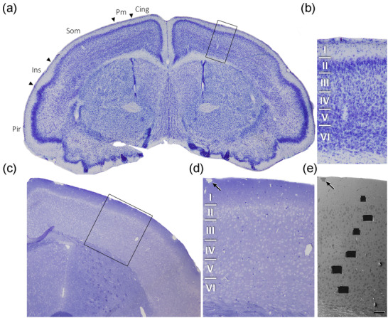
Correlative light‐electron microscopy study of the Etruscan shrew cerebral cortex. (a) Low power photograph of a 150 µm Nissl stained coronal vibratome section of the Etruscan shrew brain. The delimitation of cortical areas and layers is based on Naumann et al. (2012). (b) Higher magnification of the boxed area in (a), showing the laminar pattern of Som cortex (layers 1 to 6 are indicated). (c) 1 µm‐thick semithin section stained with toluidine blue. (d) Higher magnification of the boxed area in (c), showing delimitated layers based on the staining pattern. The semithin section is adjacent to the block for FIB/SEM imaging. (e) SEM image illustrating the block surface with trenches made in the neuropil (one per layer). Arrows in (d) and (e) point to the same blood vessel, showing that the exact location of the region of interest was accurately determined. Scale bar shown in (e) represents 200 µm in (a), 60 µm in (b), 105 µm in (c), 50 µm in (d) and 55 µm in (e). Cing—Cingulate Cortex; Pm—Parietal Medial Cortex; Som—Somatosensory Cortex; Ins—Insular Cortex; Pir—Piriform Cortex.

2.3. Three‐dimensional electron microscopy

Images were obtained from the neuropil, which is where the vast majority of synapses are found (DeFelipe et al., 1999). The neuropil is composed of axons, dendrites and glial processes, so the samples did not contain cell somata, proximal dendrites in the immediate vicinity of the soma, or blood vessels.

Three‐dimensional brain tissue samples of the somatosensory cortex were obtained using a Neon40 EsB electron microscope (Carl Zeiss NTS GmbH, Oberkochen, Germany). This instrument combines a high‐resolution field emission SEM column with a focused gallium ion beam (FIB), which mills the sample surface, removing thin layers of material on a nanometer scale. After removing each slice (20 nm thick), the milling process was paused, and the freshly exposed surface was imaged with a 1.7 kV acceleration potential using the in‐column energy selective backscattered (EsB) electron detector. The milling and imaging processes were sequentially repeated, and long series of images were acquired through a fully automated procedure (Merchan‐Perez et al., 2009), thus obtaining a stack of images that represented a three‐dimensional sample of the tissue (see an example of a series of images in Supplementary video). Eighteen samples (stacks of images) of the neuropil from the somatosensory cortex were obtained in the six layers (one sample per layer and per animal, in layers 1, 2, 3, 4, 5, and 6).

Image resolution in the xy plane was 4.652 nm/pixel. Resolution in the z axis (section thickness) was 20 nm and image sizes were 2048 × 1536 pixels. These parameters allowed a field of view where synaptic junctions could be clearly identified, within a reasonable image acquisition timeframe (approximately 12 h per stack of images). The number of sections per stack ranged from 200 to 301 (accumulative total: 4335 sections). The volumes of the stacks ranged from 339 to 527 µm³, and a total volume of 7460 µm³ was sampled (considering the corrected volume that accounted for tissue shrinkage). All measurements were corrected for the tissue shrinkage that occurs during the processing of sections (Merchan‐Perez et al., 2009). To estimate the shrinkage in our samples, we photographed and measured the area of the brain sections with ImageJ (ImageJ 1.51; NIH, USA), both before and after processing for electron microscopy. The section area values after processing were divided by the values before processing to obtain the volume, area, and linear shrinkage factors (Oorschot et al., 1991), yielding correction factors of 0.803, 0.864, and 0.929, respectively. Nevertheless, in order to compare with previous studies—in which no correction factors had been included or such factors were estimated using other methods—in the present study, we provide both sets of data.

2.4. Three‐dimensional analysis of synapses

Stacks of images obtained by the FIB/SEM were analyzed using EspINA software (EspINA Interactive Neuron Analyzer, 2.1.9; https://cajalbbp.es/espina/). As previously discussed (Merchan‐Perez et al., 2009), there is a consensus for classifying cortical synapses into asymmetric synapses (AS; or type I) and symmetric synapses (SS; or type II). The main characteristic distinguishing these synapses is the prominent or thin postsynaptic density, respectively (Gray, 1959; Colonnier, 1968; Peters et al., 1991; Figures 2 and 3). Also, these two types of synapses are associated with different functions: AS are mostly glutamatergic and excitatory, while SS are mostly GABAergic and inhibitory (Ascoli et al., 2008; DeFelipe & Fariñas, 1992; Houser et al., 1984). Nevertheless, in single sections, the synaptic cleft and the pre‐ and postsynaptic densities are often blurred if the plane of the section does not pass at right angles to the synaptic junction. Since the software EspINA allows navigation through the stack of images, it was possible to unambiguously identify every synapse as AS or SS, based on the thickness of the postsynaptic density (PSD) (Merchan‐Perez et al., 2009).

FIGURE 2.

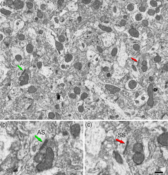
Images of neuropil in layer 3 of Etruscan shrew somatosensory cortex obtained by FIB/SEM. (a) Two synapses are indicated as examples of asymmetric (AS, green arrow) and symmetric (SS, red arrow) synapses. (b, c) Higher magnification of AS (b) and SS (c) indicated in (a). Synapse classification was based on the examination of the full sequence of serial images (see Figure 3). Scale bar in (c) represents 500 nm in (a), and 250 nm in (b) and (c).

FIGURE 3.

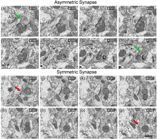
Sequence of FIB/SEM serial images of an AS (a–h) and an SS (i–p) indicated in Figure 2. Numbers on the top right of each panel indicate the number of each section from a stack of serial sections. Synapse classification was based on the examination of full sequences of serial images, see Section 2.4 for further details. Asterisks (in d–h) indicate a spine apparatus in a postsynaptic dendritic spine head. Scale bar shown in (p) represents 500 nm in (a–p).

EspINA provided the 3D reconstruction of every synapse and allowed the application of an unbiased 3D counting frame (CF), which is a rectangular prism enclosed by three acceptance planes and three exclusion planes marking its boundaries. All synapses within the CF were counted, as were those intersecting any of the acceptance planes, while synapses that were outside the CF, or intersecting any of the exclusion planes, were not counted (Figure 4). Thus, the number of synapses per unit volume was calculated directly by dividing the total number of synapses counted by the volume of the CF (Merchan‐Prez et al., 2009), in all 18 stacks of images.

FIGURE 4.

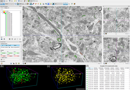
Screenshot of the EspINA software user interface. (a) In the main window, the sections are viewed through the xy plane (as obtained by FIB/SEM microscopy). The other two orthogonal planes, yz and xz, are also shown in adjacent windows (on the right). (b) 3D reconstructions of segmented AS (green) and SS (red). (c) Computed SAS for each reconstructed synapse (yellow). (d) Table of synaptic 3D morphometric data from AS automatically obtained by EspINA software. Scale bar in (c) represents 5 µm in (b) and (c).

Synaptic size was calculated using the Synaptic Apposition Surface (SAS), which was automatically extracted by EspINA (Figure 4c). The SAS represents both the active zone (presynaptic density) and the PSD, resulting in a functionally relevant measurement of the synaptic size (Morales et al., 2013). Estimations of the SAS were made for each individually 3D reconstructed complete synapse in all FIB/SEM stacks, with the SAS area providing a reliable synaptic size measurement.

EspINA also allowed us to visualize each of the reconstructed synapses in 3D and to detect the possible presence of perforations or deep indentations in their perimeters. Regarding the shape of the PSD, the synapses were classified according to the categories proposed by Santuy et al. (2018a): macular (disk‐shaped PSD); perforated (with one or more holes in the PSD); horseshoe‐shaped (with an indentation); and fragmented (two or more disk‐shaped PSDs with no connection between them).

In addition, to identify the postsynaptic targets of the axon terminals, we navigated through the image stacks using EspINA to determine whether the postsynaptic element was a dendritic spine (spine, for simplicity) or a dendritic shaft. As previously described in Domínguez‐Alvaro et al. (2021), unambiguous identification of spines requires the spine to be visually traced to the parent dendrite, in which case we refer to them as “complete spines.” When synapses are established on a spine‐shaped postsynaptic element whose neck cannot be followed to the parent dendrite, we identify these elements as “incomplete spines.” These incomplete spines were identified based on their size and shape, the lack of mitochondria and the presence of a spine apparatus (a term coined by Peters et al., 1991)—or because they were filled with a characteristic fluffy material (used to describe the fine and indistinct filaments present in the spines) (see also del Río & DeFelipe, 1995).

2.5. Spatial distribution analysis of synapses

In addition, the positions of the centers of gravity (centroids) of each reconstructed synapse were also calculated by EspINA in all FIB/SEM stacks of images.

To analyze the spatial distribution of synapses, Spatial Point Pattern analysis was performed on the centroids as described elsewhere (Antón‐Sánchez et al., 2014; Merchán‐Pérez et al., 2014). Briefly, we compared the actual position of synapse centroids with the Complete Spatial Randomness (CSR) model—a random spatial distribution model which defines a situation where a point is equally likely to occur at any location within a given volume. To do this, we generated an envelope simulating 99 instances of random distributions of the same number of points as our experimental sample.

Then, for each of the 18 FIB/SEM stacks of images, we calculated three functions commonly used for spatial point pattern analysis: F, G, and K functions. When these functions lay within the envelope, we concluded that the distributions of synapses were random. Otherwise, the distribution of points may be clustered (when points are closer to each other than expected by chance) or regular (when points tend to separate from each other further that expected by chance). The F function, also known as the empty space function or the point‐to‐event distribution, is the cumulative distribution of distances between the centroids of synapses and the closest point in a regularly spaced grid of points superimposed over the sample. The G function, also called the nearest‐neighbor distance cumulative distribution function or the event‐to‐event distribution, is the cumulative distribution of distances between each centroid and its nearest neighbor. The K function is also called the reduced second moment function or Ripley's function. An estimation of the K function is given by the mean number of points within a sphere of increasing radius centered on each sample centroid. See Merchan‐Perez et al. (2014) and Anton‐Sanchez et al. (2014) for examples of studies in which this methodology was used to investigate the spatial distribution of synapses. The present study was carried out using the Spatstat package and R Project program (Baddeley et al., 2015).

2.6. Statistical analysis

To study whether there were significant differences between synaptic characteristics among the different layers, we performed a multiple mean comparison test on the 18 samples of the six cortical layers. If the necessary assumptions for ANOVA were not satisfied (the normality and homoscedasticity criteria were not met), we used the Kruskal–Wallis test (KW) and the Mann–Whitney test (MW) for pair‐wise comparisons. χ² tests were used for contingency table analysis. Frequency distribution analysis of the SAS area was performed using Kolmogorov–Smirnov (KS) nonparametric test. Statistical studies were performed with the GraphPad Prism statistical package (Prism 9.00 for Windows, GraphPad Software Inc., USA), Spatstat package for R Project program (Baddeley et al., 2015) and Easyfit Professional 5.5 (MathWave Technologies).

3. RESULTS

The following results were obtained in the neuropil, so they represent synapses located among cell bodies, excluding perisomatic synapses and synapses established on thick proximal dendritic trunks.

3.1. Synaptic density

The number of synapses per volume was calculated in the 18 stacks of images obtained from 3 animals, in 6 layers per animal. A total of 9033 synapses were individually identified and reconstructed in 3D. Of these, 7239 synapses were analyzed after discarding synapses that were truncated by the margins of the stack or those touching the exclusion edges of the counting frame (CF). Summing all the CFs that were applied yielded a total volume of 5578 µm³ (Table 1). The synaptic density values were obtained by dividing the total number of synapses included within each CF by its total volume. Since the synapses were fully reconstructed in 3D, it was possible to classify them as AS and SS based on the thickness of their PSDs, allowing us to compute the densities and proportions of AS and SS in each cortical layer (Merchan‐Perez et al., 2009).

TABLE 1.

Accumulated synaptic data per animal

Animal	No. of AS	No. of SS	Total no. of synapses	% AS (mean ± SD)	% SS (mean ± SD)	Total Analyzed Volume (µm3)	No. of AS/µm3 (mean ± SD)	No. of SS/µm3 (mean ± SD)	Total no. of synapses/ µm3 (mean ± SD)	Area of SAS AS (nm2; mean ± SE)	Area of SAS SS (nm2; mean ± SE)	Intersynaptic distance (nm; mean ± SD)
MS1	1750	249	1999	87.4 ± 5.3	12.6 ± 5.3	1831	0.95 ± 0.22	0.13 ± 0.05	1.08 ± 0.21	77,249 ± 5557	63,774 ± 3950	629 ± 51
						(1469)	(1.19 ± 0.27)	(0.16 ± 0.06)	(1.35 ± 0.26)	(66,699 ± 4798)	(55,064 ± 3411)	(584 ± 47)
MS2	2223	209	2432	91.4 ± 3.1	8.6 ± 3.1	1957	1.2 ± 0.4	0.10 ± 0.03	1.30 ± 0.39	70,672 ± 4102	53,290 ± 2813	574 ± 54
						(1570)	(1.49 ± 0.5)	(0.13 ± 0.04)	(1.62 ± 0.49)	(61,020 ± 3542)	(46,012 ± 2429)	(533 ± 50)
MS3	2591	217	2808	92.1 ± 1.5	7.9 ± 1.5	1790	1.43 ± 0.29	0.12 ± 0.03	1.55 ± 0.31	74,067 ± 4380	64,071 ± 5507	570 ± 51
						(1436)	(1.78 ± 0.37)	(0.15 ± 0.04)	(1.93 ± 0.39)	(63,952 ± 3782)	(55,321 ± 4755)	(529 ± 47)
Total	6564	675	7239	90.3 ± 2.5	9.7 ± 2.5	5578	1.19 ± 0.24	0.12 ± 0.01	1.31 ± 0.23	73,996 ± 3289	60,378 ± 6140	591 ± 33
						(4475)	(1.49 ± 0.29)	(0.15 ± 0.02)	(1.63 ± 0.29)	(63,890 ± 2840)	(52,133 ± 5302)	(549 ± 31)

Note: Data in parentheses are not corrected for shrinkage.

AS: asymmetric synapses; SAS: synaptic apposition surface; SE: standard error of the mean; SD: standard deviation; SS: symmetric synapses.

The overall synaptic density—obtained by averaging all layers and animals—was 1.31 synapses/µm³ (Table 1). The total synaptic density and AS density reached the highest values in layer 1 (1.70 and 1.62 synapses/µm³, respectively), and the lowest values in layer 6 (1.01 and 0.91 synapses/µm³, respectively; Figure 5a, Tables 2 and 3). Regarding SS, the density was highest in layer 3 and lowest in layer 1 (Table 2).

FIGURE 5.

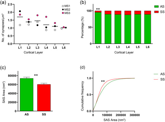
Plots of the synaptic analysis of the Etruscan shrew somatosensory cortex. (a) Mean of the overall synaptic density from each layer. Different colors correspond to each analyzed animal, as denoted in the upper right‐hand corner. (b) Proportion of AS and SS per layer expressed as percentages, showing that layer 1 was different from the other layers (χ²; p < .0001). (c) Mean SAS area per synaptic type shows larger synaptic size of AS compared to SS (MW, p = .0015). (d) Cumulative frequency distribution graph of SAS area illustrating that small SS (red) were more frequent (KS, p < .0001) than small AS (green). Asterisks indicate statistically significant differences.

TABLE 2.

Synaptic data per layer

Layer	No. of AS	No. of SS	Total no. of synapses	% AS (mean)	% SS (mean)	CFs volume (µm3)	No. of AS /µm3 (mean ± SD)	No. of SS /µm3 (mean ± SD)	Total no. of synapses/µm3 (mean ± SD)	Area of SAS AS (nm2; mean ± SE)	Area of SAS SS (nm2; mean ± SE)	Intersynaptic distance (nm; mean ± SD)
1	1462	75	1537	95.6	4.4	889 (713)	1.62 ± 0.43 (2.02 ± 0.54)	0.08 ± 0.03 (0.10 ± 0.04)	1.70 ± 0.46 (2.12 ± 0.57)	74,007 ± 9263 (63,900 ± 7998)	48,777 ± 3798 (42,116 ± 3279)	532 ± 68 (495 ± 63)
2	989	114	1103	89.9	10.1	810 (650)	1.25 ± 0.2 (1.56 ± 0.25)	0.14 ± 0.03 (0.17 ± 0.04)	1.38 ± 0.17 (1.73 ± 0.21)	83,645 ± 3338 (72,221 ± 2882)	56,586 ± 1630 (48,858 ± 1407)	575 ± 24 (534 ± 23)
3	1414	171	1585	89.1	10.9	1103 (885)	1.30 ± 0.31 (1.62 ± 0.39)	0.16 ± 0.01 (0.19 ± 0.01)	1.46 ± 0.32 (1.81 ± 0.4)	72,549 ± 5111 (62,641 ± 4413)	57,678 ± 4220 (49,801 ± 3644)	564 ± 38 (524 ± 36)
4	872	114	986	88.2	11.8	886 (695)	1.08 ± 0.44 (1.34 ± 0.55)	0.13 ± 0.04 (0.16 ± 0.05)	1.21 ± 0.44 (1.50 ± 0.55)	75,505 ± 2688 (65,194 ± 2321)	56,642 ± 389 (48,906 ± 336)	608 ± 35 (565 ± 33)
5	921	94	1015	89.7	10.3	912 (732)	1.00 ± 0.24 (1.24 ± 0.31)	0.11 ± 0.03 (0.13 ± 0.04)	1.10 ± 0.22 (1.37 ± 0.27)	79,242 ± 5977 (68,420 ± 5161)	71,149 ± 9078 (61,432 ± 7838)	635 ± 67 (590 ± 62)
6	906	107	1013	89.4	10.6	997 (800)	0.91 ± 0.05 (1.13 ± 0.06)	0.11 ± 0.1 (0.13 ± 0.01)	1.01 ± 0.04 (1.26 ± 0.05)	59,028 ± 3943 (50,966 ± 3405)	71,439 ± 4786 (61,683 ± 4132)	631 ± 43 (587 ± 40)
1–6	6564	675	7239	91.5	8.5	5578 (4475)	1.19 ± 0.26 (1.49 ± 0.32)	0.12 ± 0.03 (0.15 ± 0.03)	1.31 ± 0.25 (1.63 ± 0.32)	73,996 ± 3411 (63,890 ± 2945)	60,378 ± 3690 (52,133 ± 3186)	591 ± 41 (549 ± 38)

Note: Data in parentheses are not corrected for shrinkage.

AS: asymmetric synapses; CF: counting frame; SAS: synaptic apposition surface; SE: standard error of the mean; SD: standard deviation; SS: symmetric synapses.

TABLE 3.

Synaptic data per layer and animal

Layer	Animal	No. of AS	No. of SS	Total no. of synapses	CF volume (µm3)	No. of AS /µm3	No. of SS /µm3	No. of synapses/µm3	Area of the SAS of AS (nm2; mean ± SE)	Area of the SAS of SS (nm2; mean ± SE)	Distance to the nearest neighbor (nm; mean)
1	MS1	267	10	277	233 (187)	1.15 (1.43)	0.04 (0.05)	1.19 (1.48)	92,532 ± 5536 (79,895 ± 4780)	56,229 ± 17,270 (48,550 ± 14,912)	607 (564)
	MS2	346	56	402	222 (178)	1.99 (2.47)	0.08 (0.10)	2.06 (2.57)	64,930 ± 2489 (56,062 ± 2149)	43,780 ± 6619 (37,801 ± 5715)	474 (440)
	MS3	446	55	501	434 (348)	1.74 (2.17)	0.11 (0.14)	1.85 (2.31)	64,560 ± 2090 (55,743 ± 1804)	46,323 ± 4737 (39,997 ± 4090)	517 (480)
2	MS1	250	58	308	330 (265)	1.05 (1.31)	0.17 (0.21)	1.22 (1.52)	77,887 ± 3077 (67,250 ± 2657)	58,300 ± 3510 (50,338 ± 4411)	602 (559)
	MS2	184	36	220	262 (210)	1.25 (1.56)	0.14 (0.17)	1.39 (1.73)	83,599 ± 3510 (72,182 ± 3031)	53,328 ± 3637 (46,045 ± 4588)	569 (529)
	MS3	257	34	291	218 (175)	1.45 (1.80)	0.10 (0.13)	1.55 (1.93)	89,448 ± 3637 (77,232 ± 3140)	58,128 ± 5873 (50,190 ± 5071)	554 (515)
3	MS1	441	17	458	362 (291)	1.23 (1.53)	0.15 (0.19)	1.38 (1.72)	81,420 ± 2811 (70,301 ± 2427)	61,116 ± 2468 (52,769 ± 4457)	569 (529)
	MS2	327	36	363	405 (325)	1.03 (1.29)	0.15 (0.18)	1.18 (1.47)	72,512 ± 2468 (62,609 ± 2131)	49,283 ± 1998 (42,553 ± 3061)	599 (556)
	MS3	418	60	478	336 (269)	1.64 (2.04)	0.17 (0.21)	1.81 (2.25)	63,716 ± 1998 (55,014 ± 1725)	62,635 ± 4534 (54,081 ± 3914)	523 (486)
4	MS1	283	24	307	353 (283)	0.71 (0.88)	0.16 (0.20)	0.87 (1.09)	70,369 ± 3131 (60,758 ± 2704)	56,759 ± 2811 (49,008 ± 3332)	621 (577)
	MS2	391	30	421	295 (237)	0.96 (1.19)	0.08 (0.10)	1.04 (1.30)	79,449 ± 2811 (68,599 ± 2427)	55,917 ± 2736 (48,280 ± 5886)	635 (590)
	MS3	363	42	405	217 (174)	1.56 (1.94)	0.15 (0.18)	1.71 (2.13)	76,698 ± 2736 (66,224 ± 2362)	57,249 ± 4820 (49,431 ± 4161)	568 (528)
5	MS1	754	48	802	251 (201)	0.73 (0.91)	0.14 (0.18)	0.88 (1.09)	87,083 ± 4144 (75,190 ± 3578)	80,928 ± 2258 (69,876 ± 9054)	711 (661)
	MS2	316	22	338	377 (302)	1.04 (1.29)	0.08 (0.10)	1.12 (1.39)	67,506 ± 2258 (58,287 ± 1950)	53,011 ± 2612 (45,771 ± 6598)	585 (544)
	MS3	550	56	606	284 (228)	1.22 (1.52)	0.10 (0.12)	1.32 (1.64)	83,137 ± 2612 (71,783 ± 2255)	79,508 ± 11,278 (68,649 ± 9737)	609 (566)
6	MS1	339	32	371	301 (241)	0.85 (1.06)	0.11 (0.14)	0.97 (1.21)	54,205 ± 2528 (46,802 ± 2183)	69,309 ± 1973 (59,843 ± 7435)	664 (617)
	MS2	346	28	374	395 (317)	0.92 (1.14)	0.11 (0.13)	1.02 (1.28)	56,034 ± 1973 (48,381 ± 1704)	64,423 ± 2453 (55,625 ± 6337)	583 (542)
	MS3	286	31	317	301 (242)	0.95 (1.18)	0.10 (0.13)	1.05 (1.31)	66,843 ± 2453 (57,715 ± 2118)	80,585 ± 9259 (69,580 ± 7995)	647 (601)

Note: Data in parentheses are not corrected for shrinkage.

AS: asymmetric synapses; SAS: synaptic apposition surface; SE: standard error of the mean; SS: symmetric synapses.

The general proportion of AS:SS, computed for all animals and layers collected was approximately 90:10 (Tables 1 and 2). Although no differences in the AS:SS ratio were found between animals, comparison among layers revealed a statistically significant difference in layer 1 (χ²; p < .0001), which displayed a higher proportion of AS than the other layers (96% AS and 4% SS; Tables 2 and 3; Figure 5b).

3.2. Three‐dimensional spatial synaptic distribution

To analyze the spatial distribution of the synapses, the actual position of each of the synapses in each stack of images was compared with a random spatial distribution model (Complete Spatial Randomness, CSR). For this, the functions G, K, and F were calculated in the 18 stacks (Figure 6). We found that in half of the stacks (9 out 18) the spatial distribution of synapses was compatible with a random distribution. In the other half of the samples, a slight tendency for a regular pattern was detected by the G function, which identified slightly larger distances to the nearest neighbor than those expected by chance (Figure 6).

FIGURE 6.

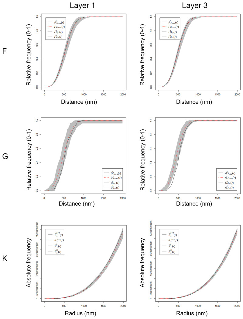
Analysis of the 3D synaptic spatial distribution in somatosensory cortex from the Etruscan shrew. Red dashed traces correspond to a theoretical homogeneous Poisson process for each function (F, G, K). The black continuous traces correspond to the experimentally observed function in the sample. The shaded areas represent the envelopes of values calculated from a set of 99 simulations. Plots show a distribution which fits into a Poisson function, but the experimental function from layer 3 for the G‐function is partially out of the envelope. Plots obtained in layer 1 and layer 3 from animal MS1.

The mean distance from each synapse centroid to its nearest neighboring synapse within the counting frame was also calculated. Synapses that were closer to the boundaries of the counting frame than to any other synapse were excluded from the calculations, since their nearest neighbor could be placed outside the counting frame at an unknown distance (Baddeley et al., 1993; Illian et al., 2007). The estimated intersynaptic distance was 591 ± 33 nm (mean ± SD) for all animals and layers. These measurements were calculated separately per layer, yielding the highest value in layer 6 (631 ± 43 nm) and the lowest in layer 1 (532 ± 68 nm; Tables 2 and 3), although the differences were not statistically significant (KS, p < .05).

3.3. Synaptic size

The study of the synaptic size was carried out analyzing the area of the SAS of each 3D reconstructed synapse (n = 7239) in the FIB/SEM stacks (Figure 4c). To characterize the distribution of SAS area data, we performed goodness‐of‐fit tests to find the theoretical probability density functions that best fitted the empirical distributions of SAS areas in each layer and in all layers pooled together. We found that the best fit corresponded to log‐normal distributions (Figure 7). These log‐normal distributions, with some variations in the location (µ) and scale (σ) parameters (Table 4), were found in all layers for both AS and SS, although the fit was better for AS than for SS, probably due to the smaller number of SS.

FIGURE 7.

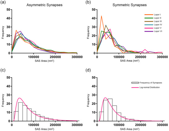
Frequency histograms of SAS areas and their corresponding best‐fit probability density functions. (a, b) Frequency histograms of SAS areas in the six cortical layers are represented for AS and SS in a and b, respectively. (c, d) Frequency histograms (white bars) and best‐fit distributions of the theoretical probability synaptic density functions (magenta traces) have been represented. The best‐fit probability functions were log‐normal distributions. Curve fitting was always better for AS (c) than for SS (d), probably because of the smaller sample size of SS (Table 4). The parameters µ and σ of the log‐normal curves are shown in Table 4.

TABLE 4.

Area of the SAS data distribution in the six cortical layers

	AS			SS
	n	µ	σ	n	µ	σ
Layer 1	1462	10.79	0.90	75	10.50	0.73
Layer 2	989	11.05	0.80	114	10.75	0.65
Layer 3	1414	10.91	0.79	171	10.80	0.59
Layer 4	872	11.03	0.68	114	10.81	0.56
Layer 5	921	11.02	0.73	94	10.93	0.71
Layer 6	906	10.74	0.74	107	10.93	0.72
Layers 1–6	6564	10.91	0.80	675	10.80	0.66

Note: Number of SAS analyzed (n), the location (µ), and scale (σ) of the best‐fit log‐normal distributions.

AS: asymmetric synapses; SAS: synaptic apposition surface; SS: symmetric synapses.

The analysis of the SAS areas showed that AS were significantly larger than SS considering all layers (MW; p = .0087; Figure 5c, Tables 1, 2, 3). These differences were also found in the frequency distribution analyses (KS; p < .0001), showing that the proportion of small SAS areas were higher in SS than in AS (Figure 5d). Analysis of the SAS area per layer showed that SAS areas of AS are larger than those from SS in all layers except in layer 6, where AS had smaller values than SS (MW, p < .05, Table 2).

3.4. Synaptic shape

A total of 2681 synapses reconstructed in 3D, from all layers, were classified into four types according to their synaptic shape: macular (with a flat, disk‐shaped PSD); perforated (with one or more holes in the PSD); horseshoe (with an indentation in the perimeter of the PSD); and fragmented synapses (with two or more physically discontinuous PSDs) (Figure 8; for a detailed description, see Santuy et al., 2018a; Domínguez‐Álvaro et al., 2019). However, fragmented synapses were excluded from further analysis since only 2 AS fragmented synapses were found (less than 0.1% of all synapses), making it impossible to draw statistically reliable conclusions. Considering all cortical layers, the vast majority of the 2472 identified AS presented macular morphology (83%), followed by perforated (11.3%), and horseshoe‐shaped (5.7%). A total of 209 SS were identified—the majority of which presented macular morphology (89%), while 7.7% were perforated and 3.3% were horseshoe‐shaped. Synaptic shape data were analyzed separately for each cortical layer (Table 5; Figure 8). Similar values were found in all layers, with layer 6 showing the highest proportion of macular synapses and layer 1 the lowest (χ², p < .0001; Figure 8).

FIGURE 8.

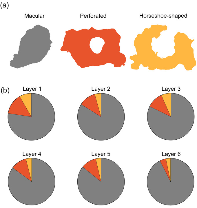
Study of the different synaptic shapes. (a) Schematic representation of the synaptic shapes: macular synapses, with a continuous disk‐shaped PSD; perforated synapses, with holes in the PSD; horseshoe‐shaped, with a tortuous perimeter with an indentation in the PSD. (b) Proportions of the different synaptic shapes of AS per cortical layer. Significantly fewer macular AS were found in layer 1, compared to the rest of the layers (χ², p <  .0001).

TABLE 5.

Proportions of the different shapes of synaptic junctions per layer

Cortical layer	Type of synapse	Macular	Perforated	Horseshoe‐shaped
Layer 1	AS	77.3% (566)	14.3% (105)	8.3% (57)
	SS	87.5% (42)	12.5% (6)	0.0% (0)
Layer 2	AS	83.9% (251)	11.7% (35)	4.3% (13)
	SS	90.5% (19)	4.8% (1)	4.8% (1)
Layer 3	AS	82.2% (410)	11.2% (56)	6.6% (33)
	SS	96.0% (48)	4.0% (2)	0.0% (0)
Layer 4	AS	85.0% (277)	11.0% (36)	4.0% (13)
	SS	87.5% (28)	9.4% (3)	3.1% (1)
Layer 5	AS	86.4% (286)	10.6% (35)	3.6% (12)
	SS	88.9% (24)	7.4% (2)	3.7% (1)
Layer 6	AS	92.5% (259)	4.3% (12)	3.2% (9)
	SS	80.6% (25)	6.5% (2)	12.9% (4)
Total	AS	83% (2050)	11.3% (279)	5.7% (137)
	SS	89% (186)	7.7% (16)	3.3% (7)

Note: Data are given as percentages with the absolute number of synapses studied in parentheses.

AS: asymmetric synapses; SS: symmetric synapses.

Analyzing all layers together and determining the proportions of the two categories (i.e., AS and SS) for each synapse shape revealed that, of the total macular synapses, 91.7% were AS and 8.3% were SS. In the case of perforated synapses, this proportion was 94.6% AS versus 5.4% SS, while in the case of the horseshoe‐shaped synapses, 95.1% were AS and 4.9% were SS. No differences in the frequencies were found considering either all layers together or each individual layer separately, regarding to the general proportion of AS:SS (χ², p > .001).

We also determined whether the shape of the synapses was related to their size. For this purpose, the area of the SAS was analyzed for each synaptic shape (Table 6). We found that analyzing all layers together and each layer separately, the mean SAS area of the macular AS was smaller than the mean area of the perforated and horseshoe‐shaped AS (KW, p < .0001). The same differences were found in the frequency distribution of the SAS area of AS (KS, p >  .01) in all layers (Figure 9). Concerning SS, the number of synapses was not sufficient to perform a robust statistical analysis for each layer, but the comparison of the SAS areas from all layers revealed that the macular SS were also, on average, smaller than the perforated and horseshoe‐shaped SS (MW, p < .0001).

TABLE 6.

Mean area of the SAS (nm²) of the macular, perforated, and horseshoe‐shaped synapses per cortical layer

Cortical layer	Type of synapse	Macular	Perforated	Horseshoe‐shaped
Layer 1	AS	45,874	139,441	119,080
		(566)	(105)	(57)
	SS	41,705	82,422	–
		(42)	(6)	(0)
Layer 2	AS	72,335	160,184	169,133
		(2519)	(35)	(13)
	SS	53,402	61,168	137,854
		(19)	(1)	(1)
Layer 3	AS	52,137	123,600	108,561
		(4109)	(56)	(33)
	SS	58,940	164,670	–
		(489)	(2)	(0)
Layer 4	AS	63,715	152,512	132,028
		(2779)	(36)	(13)
	SS	52,942	99,540	50,924
		(289)	(3)	(1)
Layer 5	AS	75,486	132,872	125,359
		(286)	(35)	(12)
	SS	74,714	153,084	53,651
		(24)	(2)	(1)
Layer 6	AS	62,397	132,917	118,328
		(260)	(12)	(9)
	SS	68,330	145,728	124,590
		(25)	(2)	(4)
Total	AS	59,260	140,825	122,331
		(2050)	(279)	(137)
	SS	59,004	109,449	100,489
		(186)	(16)	(7)

Note: All data are corrected for shrinkage. Absolute numbers of synapses are in parentheses.

AS: asymmetric synapses; SS: symmetric synapses.

FIGURE 9.

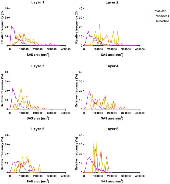
Frequency distribution plots of SAS area of AS per cortical layer. Different colors correspond to each synaptic shape, as denoted in the key. Statistical comparisons showed differences in the frequency distribution of the SAS area of macular synapses compared to perforated and horseshoe‐shaped synapses (KS, p < .0001).

3.5. Study of the postsynaptic elements

Postsynaptic targets were identified and classified as dendritic spines (including both complete and incomplete spines, as detailed above) or dendritic shafts (Figure 10). The postsynaptic elements of 2589 synapses from all cortical layers were identified; of these, 77.9% were AS established on spines, 13.9% were AS on dendritic shafts, 7.1% were SS on dendritic shafts, and 0.8% were AS on spines.

FIGURE 10.

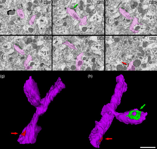
3D reconstruction of a dendritic segment from FIB/SEM serial images. (a–f) Images 121, 129, 134, 136, 140, and 155 from a stack of serial sections obtained with FIB/SEM, showing a dendritic segment partially reconstructed (in purple). An asymmetric synapse (green arrow) on a dendritic spine, and a symmetric synapse (red arrow) on the shaft are indicated. (g–h) 3D reconstructions of the same dendritic segment are displayed, after rotation about the major dendritic axis. The dendritic spine is shown establishing an asymmetric synapse (green)—and one symmetric synapse (red) on the shaft is also visible. Note that the shape of the asymmetric synapse can be identified as perforated (h). Scale bar (in h) indicates 1400 nm in a–f and 700 nm in g, h.

Considering all types of synapses established on the spines, the proportion of AS:SS was 99:1; while in those established on dendritic shafts, this proportion was 66:34. Since the overall AS:SS ratio was 90:10, the present results show that AS and SS show a “preference” for a particular postsynaptic element; that is, AS show a preference for the spines (χ², p < .0001), while the SS show a preference for the dendritic shafts (χ², p < .0001; Table 7). The same analysis was performed in each cortical layer separately, and in all the layers together, with AS showing a preference for spines (χ², p < .0001; Table 7; Figure 11) and the SS showing a preference for dendritic shafts (χ², p < .0001; Table 7).

TABLE 7.

Distribution of AS and SS on spines and dendritic shafts per cortical layer

Cortical layer	Type of synapse	On spines	On shafts	Total
Layer 1	AS	94.9% (655)	5.1% (35)	100% (690)
	SS	17.4% (8)	86.4% (39)	100% (47)
Layer 2	AS	87.1% (256)	12.9% (38)	100% (294)
	SS	4.8% (1)	95.2% (20)	100% (21)
Layer 3	AS	96.5% (469)	3.5% (17)	100% (486)
	SS	12.2% (6)	87.8% (43)	100% (49)
Layer 4	AS	75.9% (245)	24.1% (78)	100% (323)
	SS	3.1% (1)	96.9% (31)	100% (32)
Layer 5	AS	68.0% (221)	32.0% (104)	100% (325)
	SS	15.4% (4)	84.6% (22)	100% (26)
Layer 6	AS	67.0% (179)	33.0% (87)	100% (266)
	SS	3.3% (1)	96.7% (29)	100% (30)
Total	AS	84.9% (2025)	15.1% (359)	100% (2384)
	SS	10.2% (21)	89.8% (184)	100% (205)

Note: Synapses established on spines include those classified as complete and incomplete spines (as detailed in Section 2). Data are given as percentages with the absolute number of synapses studied in parentheses.

AS: asymmetric synapses; SS: symmetric synapses.

FIGURE 11.

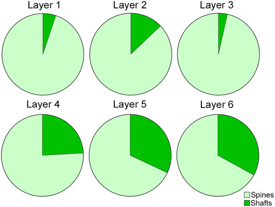
Proportions of postsynaptic targets—dendritic spines and shafts—of AS per cortical layer. AS show a significant preference for spines in all layers (χ²; p < .0001). Layers 4, 5 and 6 displayed a greater proportion of AS on spines than layers 1, 2, and 3 (χ²; p < .0001).

To determine whether there was a difference between the different cortical layers with regard to the postsynaptic elements, the distribution of the postsynaptic elements was analyzed in each cortical layer separately. Differences between layers were found regarding the proportions of AS on spines and on dendritic shafts—AS on spines were more frequent in layers 1 and 3, while AS on dendritic shafts were more frequent in layers 5 and 6 (χ², p < .0001; Table 7; Figure 11).

Additionally, we studied synaptic size regarding the postsynaptic targets. This was carried out with the data of the SAS area of each synapse whose postsynaptic element was identified. The mean SAS area of AS on dendritic shafts (68,231 nm²) was similar to the area of AS on spines (61,402 nm²; MW, p > .05). Separate analyses per cortical layer showed no differences regarding the area of the SAS from AS (Table 8). Concerning SS, the number of synapses was not sufficient to perform a robust statistical analysis for each layer, but the comparison of the SAS areas from all layers together revealed no differences between synapses established on spines and those established on dendritic shafts (MW, p = .246).

TABLE 8.

Mean area of the SAS (nm²) of the synapses on different postsynaptic targets per cortical layer

Layer	Type of synapse	On incomplete spines	On complete spines	On spines (total)	On shafts
Layer 1	AS	46,353	75,169	64,383	74,813
		(445)	(210)	(655)	(35)
	SS	54,608	36,289	57,939	44,448
		(6)	(2)	(8)	(38)
Layer 2	AS	61,498	103,722	89,943	82,645
		(158)	(98)	(256)	(38)
	SS	–	39,793	46,086	60,063
		(0)	(1)	(1)	(20)
Layer 3	AS	45,407	70,815	63,630	65,552
		(293)	(176)	(469)	(17)
	SS	48,254	55,094	57,205	65,842
		(5)	(1)	(6)	(43)
Layer 4	AS	62,828	77,026	78,536	73,935
		(159)	(86)	(245)	(78)
	SS	–	41,623	48,205	57,540
		(0)	(1)	(1)	(31)
Layer 5	AS	65,393	80,101	80,668	90,938
		(157)	(64)	(221)	(104)
	SS	33,750	51,388	49,301	82,058
		(2)	(2)	(4)	(22)
Layer 6	AS	47,169	66,410	66,454	72,073
		(84)	(95)	(179)	(87)
	SS	74,496	–	86,277	82,500
		(1)	(0)	(1)	(29)
Total	AS	54,775	78,874	71,112	79,021
		(1296)	(729)	(2025)	(359)
	SS	52,777	44,837	56,406	63,845
		(14)	(7)	(21)	(184)

Note: All data are corrected for shrinkage. Absolute numbers of synapses are in parentheses.

AS: asymmetric synapses; SS: symmetric synapses.

4. DISCUSSION

The present study constitutes the first description of the ultrastructural synaptic characteristics of the neuropil from the cerebral cortex of the Etruscan shrew. The following major results were obtained: (i) cortical synaptic density was very high, particularly in layer 1; (ii) the vast majority of synapses were excitatory—the highest proportion was found in layer 1; (iii) excitatory synapses were larger than inhibitory synapses in all layers except in layer 6; and (iv) synapses were either randomly distributed in space or showed a slight tendency for a regular pattern; (v) most synapses displayed a macular shape, and were, on average, smaller than complex‐shaped synapses (horseshoe‐shaped and fragmented); and (vi) most AS were established on dendritic spines, while most SS were established on dendritic shafts.

What follows is a discussion of the above results in comparison with data obtained from the human cerebral cortex (unless otherwise specified). From an evolutionary point of view, it is of particular interest to compare the synaptic organization of the brain of the smallest mammal with that of the much larger human brain, whose synaptic organization is thought to have reached the highest level of complexity. Fortunately, data is available from the human cerebral cortex that was obtained using the same methodology (Cano‐Astorga et al., 2021; Domínguez‐Álvaro et al., 2018; 2021) as that used in the present study, avoiding the difficulties that are inherent when comparing different studies using different approaches. Thus, similarities and differences in the synaptic organization can be directly compared to examine what characteristics are conserved in evolution.

4.1. Number of synapses and spatial distribution

Synaptic density is a useful parameter for describing synaptic organization, in terms of connectivity and functionality. In the Etruscan shrew, high densities of synapses were found in all layers of the somatosensory cortex, with a mean synaptic density of 1.31 synapses/µm³. No quantitative analysis of the synapses in the Etruscan shrew cerebral cortex has been performed previously and, thus, it is not possible to compare our results with those of others. However, the values for the synaptic density of the Etruscan shrew are almost triple those obtained in cortical samples from human temporal and entorhinal cortex using the same 3D EM method and image analysis (Cano‐Astorga et al., 2021; Domínguez‐Álvaro et al., 2021; Table 9).

TABLE 9.

Summary of synaptic data from FIB/SEM studies for comparison

Species	Brain region	Layer	Reference	No., sex (age)	No. of AS	No. of SS	Total no. of synapses	AS:SS (percentage)	Total no. of synapses/µm3	Area of SAS AS (nm2; mean)	Area of SAS SS (nm2; mean)	Intersynaptic distance (nm; mean)
Etruscan Shrew	Somatosensory cortex	1—6	Present study	3 M (adult)	6564	675	7239	90:10	1.31 (1.63)	73,996 (63,890)	60,378 (52,133)	591 (549)
Human	Middle temporal gyrus	3	Cano‐Astorga et al. (2021)	5 M; 3 F (24−53 y.o.)	4618	327	4945	93:7	0.60 (0.67)	110,243 (102,526)	73,196 (68,072)	756 (735)
Human	Entorhinal cortex	2, 3	Domínguez‐Álvaro et al. (2021)	4 M (40−63 y.o.)	3300	267	3567	93:7	0.42 (0.47)	117,247 (109,039)	66,721 (62,051)	826 (802)

Note: Data in parentheses are not corrected for tissue shrinkage.

AS: asymmetric synapses; F: female; M: male; SAS: synaptic apposition surface; SS: symmetric synapses.

The highest synapse density was found in layer 1 (1.70 synapses/µm³; Table 2), which has a very low density of neurons (Figure 1). In addition, the thickness of layer 1 in the Etruscan shrew somatosensory cortex represents about 20% of the total cortical thickness (Naumann et al., 2012). That is, in the Etruscan shrew, given the high synaptic density in layer 1 and its relatively large proportion, this layer greatly contributes to the total number of synapses in the somatosensory cortex.

The present study was carried out in adult Etruscan shrews of different ages, but we did not consider possible effects of age. For example, in aged rhesus monkey, a lower number of synapses have been reported in prefrontal cortex related to a cognitive decline; however, other studies in rats and monkeys have shown no evidence of synaptic loss with age in mesial temporal lobe structures (reviewed in Morrison & Baxter, 2012).

In the present study, the AS:SS ratio was 90:10 (ranging from 88:12 to 96:4), which is within the range of the cortical values reported from other species. The percentage of AS and SS varies between 80−95% and 20−5%, respectively—in all the cortical layers, cortical areas and species examined so far using transmission electron microscopy (Beaulieu & Colonnier, 1985; Bourne & Harris, 2011; DeFelipe, 2011, 2015; DeFelipe et al., 2002; Megías et al., 2001) or FIB/SEM (Cano‐Astorga et al., 2021; Domínguez‐Álvaro et al., 2018, 2021; Montero‐Crespo et al., 2020; Santuy et al., 2018a). However, layer 1 of the Etruscan shrew displays the highest proportion of AS (approximately 96:4, AS:SS) compared to other cortical layers where this proportion was similar (89:11). This suggests that there is a layer‐specific excitatory‐inhibitory balance.

Regarding the spatial organization of synapses, we found that the synapses either fitted to a random distribution in the neuropil or showed a slight tendency for a regular pattern, where points tend to separate from each other more than expected by chance. In the latter case, this may be because the spatial statistical functions are applied to the centers of gravity or centroids of the synaptic junction. However, it is important to take into account that synaptic junctions cannot overlap, and thus the minimum distances between their centroids are limited by the sizes of the synaptic junctions themselves, resulting in a slightly dispersed distribution of the centroids. This type of spatial distribution, which is based on a random distribution with a minimum‐spacing rule, has also been found in the rat somatosensory cortex (Merchan‐Perez et al., 2014; Anton‐Sanchez et al., 2014) and several regions of the human brain including frontal cortex, transentorhinal cortex, entorhinal cortex, temporal cortex and CA1 hippocampal field (Blazquez‐Llorca et al., 2013; Cano‐Astorga et al., 2021; Domínguez‐Álvaro et al., 2018; 2021; Montero‐Crespo et al., 2020). As proposed by Merchan‐Perez et al. (2014), in a random distribution, a synapse could be formed anywhere in space where an axon terminal and a dendritic element may touch, provided this particular spot is not already occupied by a pre‐ existing synapse. However, spatial randomness does not necessarily mean non‐specific connections. Spatial specificity in the neocortex may be scale‐dependent. It is well known that, at the macroscopic and mesoscopic scales, the mammalian nervous system is a highly ordered and stereotyped structure where connections are established in a highly specific and ordered way. Even at the microscopic level, it is clear that different areas and layers of the cortex receive specific inputs. However, at the ultrastructural level, synapses are often observed to be distributed in a nearly random pattern. This could mean that, as the axon terminals reach their destination, the spatial resolution achieved by them is fine enough to find a specific cortical layer, but not sufficiently fine to make a synapse on a particular target, such as a specific dendritic branch or dendritic spine within a layer. Therefore, the present results indicating the random spatial distribution of synapses are in line with the proposed widespread “rules” of the synaptic organization of the mammalian cerebral cortex.

4.2. Synaptic size and shape

It has been proposed that synaptic size is directly related to neurotransmitter release probability, synaptic strength, efficacy and plasticity (e.g., Ganeshina et al., 2004a; Holderith et al., 2012; Matz et al., 2010; Montes et al., 2015; Nusser et al., 1998; Südhof, 2012; Tarusawa et al., 2009). Hence, the analysis of the synaptic size provides useful information about the synaptic function of a particular brain region.

In the present study, we used the values obtained from the SAS, which is equivalent to the interface between the active zone and the postsynaptic density (Morales et al., 2013). Thus, investigating SAS area is an appropriate approach to analyze the synaptic size (Morales et al., 2013). Analysis of the somatosensory cortex of the Etruscan shrew has shown that SAS area was larger in AS than in SS (Figure 5), which is similar to previous data obtained in other cortical areas and species using the same method (Cano‐Astorga et al., 2021; Domínguez‐Álvaro et al., 2021; Montero‐Crespo et al., 2020). In addition, the SAS area of both types of synapses (asymmetric and symmetric) follows log‐normal distributions, as do many other neuroanatomical and physiological variables such as synaptic strength, axonal width, and corticocortical connection density (Buzsáki & Mizuseki, 2014; Markov et al., 2014; Robinson et al., 2021).

However, we observed that the SAS area for AS was much smaller (73,996 nm²) compared to that found in the human temporal cortex and entorhinal cortex (110,243 nm² and 117,247 nm², respectively; Table 9). However, the SAS area for SS was similar to that found in other species and cortical regions (Table 9), which may indicate that SS are more homogeneous across species than AS (Santuy et al., 2018b).

Moreover, the present results show that most synapses presented a macular shape, which is in line with previous reports in other brain areas and species (Calì et al., 2018; Cano‐Astorga et al., 2021; Domínguez‐Álvaro et al., 2019, 2021; Geinisman et al., 1987; Hsu et al., 2017; Jones et al., 1991; Montero‐Crespo et al., 2020; Santuy et al., 2018a). The lowest and the highest proportions of macular synapses were found in layer 1 and layer 6, respectively, which suggests specific layer‐dependent differences. In all layers, complex‐shaped synapses were, on average, larger than macular ones. It has been widely reported that complex‐shaped synapses have more AMPA and NMDA receptors than macular synapses (Ganeshina et al., 2004a, 2004b; Lüscher et al., 2000; Montes et al., 2015). Therefore, macular synapses may constitute a population of synapses with more dynamic functionality than complex synapses.

It should be kept in mind that the SAS area of the AS is rather variable (Table 3). Larger and more complex synapses have been proposed to have more receptors in their postsynaptic elements than small synapses, and are thought to constitute a synaptic population with long‐lasting memory‐related functionality (e.g., Ganeshina et al., 2004a, 2004b; Geinisman et al., 1993; Lüscher et al., 2000; Toni et al., 2001)—whereas, small active zones may play a special role in synaptic plasticity (Kharazia & Weinberg, 1999). Thus, the presence of relatively small AS in the neuropil of the somatosensory cortex of the Etruscan shrew may indicate a lower release probability, synaptic strength and efficacy. In fact, hippocampal mossy fibers in Etruscan shrew have shown lower long‐ and short‐term plasticity, as well as reduced expression of synaptotagmin‐7 (a key synaptic protein in the regulation of presynaptic function) compared to mice (Beed et al., 2020). In this regard, it has been shown that mammalian brain synapses contain thousands of synaptic proteins resulting a high level of synapse diversity (Biederer et al., 2017; Zhu et al., 2018), which may result in synaptic species‐specific differences (Curran et al., 2021). Thus, it is likely that molecular characterization of the synaptic proteins in the Etruscan shrew cortex may reveal additional specific synaptic characteristics.

4.3. Postsynaptic targets

The present results show that AS have a clear preference for dendritic spines, since 85% of AS are established on spines (axospinous). SS, on the contrary, show a preference for dendritic shafts, as 90% of SS are established on dendritic shafts (axodendritic). Given that AS outnumber SS in a proportion of 90:10, the proportion of AS:SS established on spines is 99:1. Moreover, AS also predominate over SS on dendritic shafts, although the proportion is more evenly balanced at 66:34.

In other rodents, the percentage of AS established on spines is similar to the Etruscan shrew—for example, in the somatosensory cortex of the young rat (Santuy et al., 2018b) and of the adult mouse (Calì et al., 2018), where 84% and 86% of AS are axospinous, respectively. These percentages are lower in the human temporal cortex, where 75% of AS are axospinous (Cano‐Astorga et al., 2021), whereas in the entorhinal cortex this value was 57% (Domínguez‐Álvaro et al., 2021). Numerous publications have also shown a clear preference of glutamatergic axons (forming AS) for spines and GABAergic axons (forming SS) for dendritic shafts in a variety of cortical regions and species (reviewed in DeFelipe et al., 2002).

In addition, we have found remarkable differences between cortical layers, showing maximum proportions of AS on spines in layers 1 and 3 (95% and 97%, respectively) and minimum proportions in layers 5 and 6 (68% and 67%, respectively). The higher proportion of AS on spines might be related to the higher proportion of AS found in layer 1. It is possible that layers with more axospinous AS contain a higher proportion of dendritic spines, but this would need to be further examined using other methods. Therefore, differences in the proportion of AS on spines might represent another microanatomical specialization of the cortical layers. Whether these laminar differences are also found in other cortical areas and species remains to be elucidated using the same methodological approaches.

Differences between cortical layers and species regarding the targets of SS are more difficult to interpret because of the scarcity of SS. Nevertheless, the present data do come from a relatively large number of serially reconstructed SS (n = 205), which is similar to other data sets obtained in our laboratory in other species. In the present study, we have also observed that the majority of SS (89.8%) were established on dendritic shafts, whereas in the human temporal and entorhinal cortex, this proportion was 85% and 83%, respectively (176 SS and 254 SS were analyzed, respectively; Cano‐Astorga et al., 2021; Domínguez‐Álvaro et al., 2021). Furthermore, a lower percentage of axodendritic SS has been reported in the young rat somatosensory cortex, in which 75% of 574 serially reconstructed SS were axodendritic (Santuy et al., 2018b). Thus, GABAergic synapses appear to be organized differently in different species.

4.4. Layer‐specific differences

In general, the structure of cortical layer 1 is highly conserved across cortical areas and mammalian species and it shows distinctive characteristics. It has sparse neurons, which are GABAergic interneurons (Schuman et al., 2019), and most of its volume is occupied by neuropil (Alonso‐Nanclares et al., 2008; Santuy et al., 2018c). Layer 1 is the predominant input layer for top‐down information, relayed by abundant projections that provide signals to the tuft branches of the pyramidal neurons (reviewed in Schuman et al., 2021). In particular, layer 1 receives axons from the thalamus and other cortical areas (corticocortical connections), as well as from local neurons from deeper layers (Muralidhar et al., 2014; Schuman et al., 2021). It has been proposed that layer 1 mediates the integration of contextual and cross‐modal information in top‐down signals with the input specific to a given area, enabling flexible and state‐dependent processing of feed‐forward sensory input arriving deeper in the cortical column (reviewed in Schuman et al., 2021). In addition, layer 6 also showed some particular characteristics, including the lowest synaptic density, a lower SAS area for AS than SS and a relatively low proportion of AS on spines compared to layer 1. Thus, synaptic characteristics show layer‐specific differences. However, the specific functional significance of the laminar differences in the synaptic organization of the Etruscan shrew remains to be elucidated.

Regarding the density and number of synapses, the Etruscan shrew has a high synaptic density of around 1300 × 10⁶ synapses per mm³, which is almost triple the estimated synaptic density (about 500 × 10⁶ synapses per mm³) in the human cortex. Since the estimated volume of the Etruscan shrew cerebral cortex is 10.6 mm³ (Nauman et al., 2012), the total number of synapses would be about 14,000 × 10⁶, whereas in the human cortex this number can be up to 138,000,000 × 10⁶ synapses (based on a total cortical volume of 553,000 mm³, as reported by Ribeiro et al., 2013). That is, the cortical volume of the human brain is about 50,000 times larger than the cortical volume of the Etruscan shrew, but the total number of cortical synapses in human is “only” around 20,000 times the number of synapses in the shrew. Furthermore, the synaptic junctions are about 35% smaller in the Etruscan shrew, which may be considered a relatively small difference. Thus, these differences in the number and size of synapses cannot be attributed to a brain size scaling effect, but rather to adaptations of synaptic circuits to particular functions.

In summary, a number of features of the synaptic organization of cortex of the Etruscan shrew seems to be species‐specific. However, there are certain general synaptic characteristics that are remarkably similar to those found in the human cerebral cortex including the following: (i) the vast majority of synapses are excitatory; (ii) synapses fit quite closely to a random spatial distribution; (iii) the size of synaptic junctions follows a lognormal distribution; (iv) excitatory synapses are larger than inhibitory synapses; (v) most synapses display a macular shape and are, on average, smaller than complex‐shaped synapses; and (vi) most AS are established on dendritic spines, while most SS are established on dendritic shafts. Therefore, these synaptic characteristics might be considered as basic bricks of the cortical synaptic organization in mammals.

AUTHOR CONTRIBUTIONS

Alonso‐Nanclares: formal analysis, data curation, writing—original draft preparation. González‐Soriano, Plaza‐Alonso, Cano‐Astorga: investigation, visualization. Merchan‐Perez, Rodríguez, Naumann, Brecht: Resources, investigation. DeFelipe: Conceptualization, supervision, writing—reviewing & editing, funding acquisition. All authors reviewed the final version of the article. All authors had full access to all the data in the study and take responsibility for the integrity of the data and the accuracy of the data analysis.

CONFLICT OF INTEREST

The authors declare that they have no conflict of interest.

PEER REVIEW

The peer review history for this article is available at https://publons.com/publon/10.1002/cne.25432.

Supporting information

Supplement Material

Alonso‐Nanclares, L. , Rodríguez, J. R. , Merchan‐Perez, A. , González‐Soriano, J. , Plaza‐Alonso, S. , Cano‐Astorga, N. , Naumann, R. K. , Brecht, M. , & DeFelipe, J. (2023). Cortical synapses of the world's smallest mammal: an FIB/SEM study in the Etruscan shrew. Journal of Comparative Neurology, 531, 390–414. 10.1002/cne.25432

DATA AVAILABILITY STATEMENT

Most data generated or analyzed during this study are included in the main text, the tables and the figures. Data sets used during the current study are available from the corresponding author on reasonable request.

REFERENCES

- Alonso‐Nanclares, L. , Gonzalez‐Soriano, J. , Rodriguez, J. R. , & DeFelipe, J. (2008). Gender differences in human cortical synaptic density. Proceedings of the National Academy of Sciences, 105(38), 14615–14619. 10.1073/pnas.0803652105 [DOI] [PMC free article] [PubMed] [Google Scholar]
- Amunts, K. , & Zilles, K. (2015). Architectonic mapping of the human brain beyond Brodmann. Neuron, 88(6), 1086–1107. 10.1016/j.neuron.2015.12.001 [DOI] [PubMed] [Google Scholar]
- Anjum, F. , Turni, H. , Mulder, P. G. H. , van der Burg, J. , & Brecht, M. (2006). Tactile guidance of prey capture in Etruscan shrews. Proceedings of the National Academy of Sciences, 103(44), 16544–16549. 10.1073/pnas.0605573103 [DOI] [PMC free article] [PubMed] [Google Scholar]
- Anton‐Sanchez, L. , Bielza, C. , Merchán‐Pérez, A. , Rodríguez, J.‐R. , DeFelipe, J. , & Larrañaga, P. (2014). Three‐dimensional distribution of cortical synapses: A replicated point pattern‐based analysis. Frontiers in Neuroanatomy, 8. 10.3389/fnana.2014.00085 [DOI] [PMC free article] [PubMed] [Google Scholar]
- Ascoli, G. A. , Alonso‐Nanclares, L. , Anderson, S. A. , Barrionuevo, G. , Benavides‐Piccione, R. , Burkhalter, A. , Buzsáki, G. , Cauli, B. , Defelipe, J. , Fairén, A. , Feldmeyer, D. , Fishell, G. , Fregnac, Y. , Freund, T. F. , Gardner, D. , Gardner, E. P. , Goldberg, J. H. , Helmstaedter, M. , Hestrin, S. , … Yuste, R. (2008). Petilla terminology: nomenclature of features of GABAergic interneurons of the cerebral cortex. Nature Reviews Neuroscience, 9, 557–568. 10.1038/nrn2402 [DOI] [PMC free article] [PubMed] [Google Scholar]
- Baddeley, A. J. , Moyeed, R. A. , Howard, C. V. , & Boyde, A. (1993). Analysis of a three‐dimensional point pattern with replication. Applied Statistics, 42(4), 641. 10.2307/2986181 [DOI] [Google Scholar]
- Baddeley, A. , Rubak, E. , & Turner, R. (2015). Spatial point patterns: methodology and applications with R. Chapman and Hall/CRC Press. [Google Scholar]
- Beaulieu, C. , & Colonnier, M. (1985). A laminar analysis of the number of round‐asymmetrical and flat‐symmetrical synapses on spines, dendritic trunks, and cell bodies in area 17 of the cat. The Journal of Comparative Neurology, 231(2), 180–189. 10.1002/cne.902310206 [DOI] [PubMed] [Google Scholar]
- Beed, P. , Ray, S. , Velasquez, L. M. , Stumpf, A. , Parthier, D. , Swaminathan, A. , Nitzan, N. , Breustedt, J. , Las, L. , Brecht, M. , & Schmitz, D. (2020). Species‐specific differences in synaptic transmission and plasticity. Scientific Reports, 10(1), 16557. 10.1038/s41598-020-73547-6 [DOI] [PMC free article] [PubMed] [Google Scholar]
- Biederer, T. , Kaeser, P. S. , & Blanpied, T. A. (2017). Trans‐cellular nano‐alignment of synaptic function. Neuron, 96(3), 680–696. 10.1016/j.neuron.2017.10.006 [DOI] [PMC free article] [PubMed] [Google Scholar]
- Blazquez‐Llorca, L. , Merchán‐Pérez, A. , Rodríguez, J.‐R. , & DeFelpie, J. (2013). FIB/SEM technology and Alzheimer's disease: Three‐dimensional analysis of human cortical synapses. Journal of Alzheimer's Disease, 34(4), 995–1013. 10.3233/JAD-122038 [DOI] [PubMed] [Google Scholar]
- Bourne, J. N. , & Harris, K. M. (2011). Coordination of size and number of excitatory and inhibitory synapses results in a balanced structural plasticity along mature hippocampal CA1 dendrites during LTP. Hippocampus, 21(4), 354–373. 10.1002/hipo.20768 [DOI] [PMC free article] [PubMed] [Google Scholar]
- Brecht, M. , Naumann, R. , Anjum, F. , Wolfe, J. , Munz, M. , Mende, C. , & Roth‐Alpermann, C. (2011). The neurobiology of Etruscan shrew active touch. Philosophical Transactions of the Royal Society B: Biological Sciences, 366(1581), 3026–3036. 10.1098/rstb.2011.0160 [DOI] [PMC free article] [PubMed] [Google Scholar]
- Buzsáki, G. , & Mizuseki, K. (2014). The log‐dynamic brain: How skewed distributions affect network operations. Nature Reviews Neuroscience, 15(4), 264–278. 10.1038/nrn3687 [DOI] [PMC free article] [PubMed] [Google Scholar]
- Calì, C. , Wawrzyniak, M. , Becker, C. , Maco, B. , Cantoni, M. , Jorstad, A. , Nigro, B. , Grillo, F. , De Paola, V. , Fua, P. , & Knott, G. W. (2018). The effects of aging on neuropil structure in mouse somatosensory cortex—A 3D electron microscopy analysis of layer 1. PLoS ONE, 13(7), e0198131. 10.1371/journal.pone.0198131 [DOI] [PMC free article] [PubMed] [Google Scholar]
- Cano‐Astorga, N. , DeFelipe, J. , & Alonso‐Nanclares, L. (2021). Three‐dimensional synaptic organization of layer III of the human temporal neocortex. Cerebral Cortex, 31(10), 4742–4764. 10.1093/cercor/bhab120 [DOI] [PMC free article] [PubMed] [Google Scholar]
- Colonnier, M. (1968). Synaptic patterns on different cell types in the different laminae of the cat visual cortex. An electron microscope study. Brain Research, 9(2), 268–287. 10.1016/0006-8993(68)90234-5 [DOI] [PubMed] [Google Scholar]
- Curran, O. E. , Qiu, Z. , Smith, C. , & Grant, S. G. N. (2021). A single‐synapse resolution survey of PSD95‐positive synapses in twenty human brain regions. European Journal of Neuroscience, 54(8), 6864–6881. 10.1111/ejn.14846 [DOI] [PMC free article] [PubMed] [Google Scholar]
- DeFelipe, J. (2011). The evolution of the brain, the human nature of cortical circuits, and intellectual creativity. Frontiers in Neuroanatomy, 5(29), 10.3389/fnana.2011.00029 [DOI] [PMC free article] [PubMed] [Google Scholar]
- DeFelipe, J. (2015). The anatomical problem posed by brain complexity and size: A potential solution. Frontiers in Neuroanatomy, 9(104), 10.3389/fnana.2015.00104 [DOI] [PMC free article] [PubMed] [Google Scholar]
- DeFelipe, J. , & Fariñas, I. (1992). The pyramidal neuron of the cerebral cortex: Morphological and chemical characteristics of the synaptic inputs. Progress in Neurobiology, 39(6), 563–607. 10.1016/0301-0082(92)90015-7 [DOI] [PubMed] [Google Scholar]
- DeFelipe, J. , & Fairén, A. (1993). A simple and reliable method for correlative light and electron microscopic studies. Journal of Histochemistry & Cytochemistry, 41(5), 769–772. 10.1177/41.5.8468459 [DOI] [PubMed] [Google Scholar]
- DeFelipe, J. , Marco, P. , Busturia, I. , & Merchan‐Perez, A. (1999). Estimation of the number of synapses in the cerebral cortex: Methodological considerations. Cerebral Cortex, 9(7), 722–732. 10.1093/cercor/9.7.722 [DOI] [PubMed] [Google Scholar]
- DeFelipe, J. , Alonso‐Nanclares, L. , & Arellano, J. (2002). Microstructure of the neocortex: Comparative aspects. Journal of Neurocytology, 31(3/5), 299–316. 10.1023/A:1024130211265 [DOI] [PubMed] [Google Scholar]
- del Río, M. R. , & DeFelipe, J. (1995). A light and electron microscopic study of calbindin D‐28k immunoreactive double bouquet cells in the human temporal cortex. Brain Research, 690(1), 133–140. 10.1016/0006-8993(95)00641-3 [DOI] [PubMed] [Google Scholar]
- Domínguez‐Álvaro, M. , Montero‐Crespo, M. , Blazquez‐Llorca, L. , Insausti, R. , DeFelipe, J. , & Alonso‐Nanclares, L. (2018). Three‐dimensional analysis of synapses in the transentorhinal cortex of Alzheimer's disease patients. Acta Neuropathologica Communications, 6(1), Article 1. 10.1186/s40478-018-0520-6 [DOI] [PMC free article] [PubMed] [Google Scholar]
- Domínguez‐Álvaro, M. , Montero‐Crespo, M. , Blazquez‐Llorca, L. , DeFelipe, J. , & Alonso‐Nanclares, L. (2019). 3D Electron microscopy study of synaptic organization of the normal human transentorhinal cortex and its possible alterations in Alzheimer’s disease. eNeuro, 6(4), ENEURO.0140‐19.2019. 10.1523/ENEURO.0140-19.2019 [DOI] [PMC free article] [PubMed] [Google Scholar]
- Domínguez‐Álvaro, M. , Montero‐Crespo, M. , Blazquez‐Llorca, L. , DeFelipe, J. , & Alonso‐Nanclares, L. (2021). 3D ultrastructural study of synapses in the human entorhinal cortex. Cerebral Cortex, 31(1), 410–425. 10.1093/cercor/bhaa233 [DOI] [PMC free article] [PubMed] [Google Scholar]
- Fons, R. , Stephan, H. , & Baron, G. (1984). Brains of Soricidae. Journal of Zoological Systematics and Evolutionary Research, 22(2), 145–158. 10.1111/j.1439-0469.1984.tb00653.x [DOI] [Google Scholar]
- Ganeshina, O. , Berry, R. W. , Petralia, R. S. , Nicholson, D. A. , & Geinisman, Y. (2004a). Synapses with a segmented, completely partitioned postsynaptic density express more AMPA receptors than other axospinous synaptic junctions. Neuroscience, 125(3), 615–623. 10.1016/j.neuroscience.2004.02.025 [DOI] [PubMed] [Google Scholar]
- Ganeshina, O. , Berry, R. W. , Petralia, R. S. , Nicholson, D. A. , & Geinisman, Y. (2004b). Differences in the expression of AMPA and NMDA receptors between axospinous perforated and nonperforated synapses are related to the configuration and size of postsynaptic densities. Journal of Comparative Neurology, 468(1), 86–95. 10.1002/cne.10950 [DOI] [PubMed] [Google Scholar]
- Geinisman, Y. , Morrell, F. , & de Toledo‐Morrell, L. (1987). Axospinous synapses with segmented postsynaptic densities: A morphologically distinct synaptic subtype contributing to the number of profiles of ‘perforated’ synapses visualized in random sections. Brain Research, 423(1), 179–188. 10.1016/0006-8993(87)90838-9 [DOI] [PubMed] [Google Scholar]
- Geinisman, Y. , Detoledo‐Morrell, L. , Morrell, F. , Heller, R. E. , Rossi, M. , & Parshall, R. F. (1993). Structural synaptic correlate of long‐term potentiation: Formation of axospinous synapses with multiple, completely partitioned transmission zones. Hippocampus, 3(4), 435–445. 10.1002/hipo.450030405 [DOI] [PubMed] [Google Scholar]
- Gray, E. G. (1959). Axo‐somatic and axo‐dendritic synapses of the cerebral cortex. Journal of Anatomy, 93(Pt 4), 420–433. [PMC free article] [PubMed] [Google Scholar]
- Hofman, M. A. (1988). Size and shape of the cerebral cortex in mammals. II. The cortical volume. Brain, Behavior and Evolution, 32(1), 17–26. 10.1159/000116529 [DOI] [PubMed] [Google Scholar]
- Holderith, N. , Lorincz, A. , Katona, G. , Rózsa, B. , Kulik, A. , Watanabe, M. , & Nusser, Z. (2012). Release probability of hippocampal glutamatergic terminals scales with the size of the active zone. Nature Neuroscience, 15(7), 988–997. 10.1038/nn.3137 [DOI] [PMC free article] [PubMed] [Google Scholar]
- Houser, C. R. , Vaughn, J. E. , Hendry, S. H. C. , Jones, E. G. , & Peters, A. (1984). GABA neurons in the cerebral cortex in cerebral cortex. In Jones E. G. & Peters A. (Eds.), Cerebral cortex (Vol. 2, pp. 63–89). New York: Plenum Press. [Google Scholar]
- Hsu, A. , Luebke, J. I. , & Medalla, M. (2017). Comparative ultrastructural features of excitatory synapses in the visual and frontal cortices of the adult mouse and monkey. Journal of Comparative Neurology, 525(9), 2175–2191. 10.1002/cne.24196 [DOI] [PMC free article] [PubMed] [Google Scholar]
- Illian, J. , Penttinen, A. , Stoyan, H. , & Stoyan, D. (2007). Statistical analysis and modelling of spatial point patterns: Illian/statistical analysis and modelling of spatial point patterns. John Wiley & Sons, Ltd. 10.1002/9780470725160 [DOI] [Google Scholar]
- Jones, D. G. , Itarat, W. , & Calverley, R. K. S. (1991). Perforated synapses and plasticity: A developmental overview. Molecular Neurobiology, 5(2‐4), 217–228. 10.1007/BF02935547 [DOI] [PubMed] [Google Scholar]
- Jürgens, K. D. (2002). Etruscan shrew muscle: The consequences of being small. Journal of Experimental Biology, 205(15), 2161–2166. 10.1242/jeb.205.15.2161 [DOI] [PubMed] [Google Scholar]
- Kharazia, V. N. , & Weinberg, R. J. (1999). Immunogold localization of AMPA and NMDA receptors in somatic sensory cortex of albino rat. Journal of Comparative Neurology, 412(2), 292–302. 10.1002/(SICI)1096-9861(19990920)412:2292::AID-CNE83.0.CO;2-G [DOI] [PubMed] [Google Scholar]
- Lüscher, C. , Nicoll, R. A. , Malenka, R. C. , & Muller, D. (2000). Synaptic plasticity and dynamic modulation of the postsynaptic membrane. Nature Neuroscience, 3(6), 545–550. 10.1038/75714 [DOI] [PubMed] [Google Scholar]
- Markov, N. T. , Ercsey‐Ravasz, M. M. , Ribeiro Gomes, A. R. , Lamy, C. , Magrou, L. , Vezoli, J. , Misery, P. , Falchier, A. , Quilodran, R. , Gariel, M. A. , Sallet, J. , Gamanut, R. , Huissoud, C. , Clavagnier, S. , Giroud, P. , Sappey‐Marinier, D. , Barone, P. , Dehay, C. , Toroczkai, Z. , … Kennedy, H. (2014). A weighted and directed interareal connectivity matrix for macaque cerebral cortex. Cerebral Cortex, 24(1), 17–36. 10.1093/cercor/bhs270 [DOI] [PMC free article] [PubMed] [Google Scholar]
- Matz, J. , Gilyan, A. , Kolar, A. , McCarvill, T. , & Krueger, S. R. (2010). Rapid structural alterations of the active zone lead to sustained changes in neurotransmitter release. Proceedings of the National Academy of Sciences, 107(19), 8836–8841. 10.1073/pnas.0906087107 [DOI] [PMC free article] [PubMed] [Google Scholar]
- Megías, M. , Emri, Z. , Freund, T. F. , & Gulyás, A. I. (2001). Total number and distribution of inhibitory and excitatory synapses on hippocampal CA1 pyramidal cells. Neuroscience, 102(3), 527–540. 10.1016/S0306-4522(00)00496-6 [DOI] [PubMed] [Google Scholar]
- Merchán‐Pérez, A. , Rodríguez, J.‐R. , Alonso‐Nanclares, L. , Schertel, A. , & DeFelipe, J. (2009). Counting synapses using FIB/SEM microscopy: A true revolution for ultrastructural volume reconstruction. Frontiers in Neuroanatomy, 3. 10.3389/neuro.05.018.2009 [DOI] [PMC free article] [PubMed] [Google Scholar]
- Merchán‐Pérez, A. , Rodríguez, J.‐R. , González, S. , Robles, V. , DeFelipe, J. , Larrañaga, P. , & Bielza, C. (2014). Three‐dimensional spatial distribution of synapses in the neocortex: A dual‐beam electron microscopy study. Cerebral Cortex, 24(6), 1579–1588. 10.1093/cercor/bht018 [DOI] [PMC free article] [PubMed] [Google Scholar]
- Montero‐Crespo, M. , Domínguez‐Álvaro, M. , Rondón‐Carrillo, P. , Alonso‐Nanclares, L. , DeFelipe, J. , & Blazquez‐Llorca, L. (2020). Three‐dimensional synaptic organization of the human hippocampal CA1 field. ELife, 9, e57013. 10.7554/eLife.57013 [DOI] [PMC free article] [PubMed] [Google Scholar]
- Montes, J. , Peña, J. M. , DeFelipe, J. , Herreras, O. , & Merchán‐Pérez, A. (2015). The influence of synaptic size on AMPA receptor activation: A Monte Carlo Model. PLoS ONE, 10(6), e0130924. 10.1371/journal.pone.0130924 [DOI] [PMC free article] [PubMed] [Google Scholar]
- Morales, J. , Rodríguez, A. , Rodríguez, J.‐R. , DeFelipe, J. , & Merchán‐Pérez, A. (2013). Characterization and extraction of the synaptic apposition surface for synaptic geometry analysis. Frontiers in Neuroanatomy, 7(20), 10.3389/fnana.2013.00020 [DOI] [PMC free article] [PubMed] [Google Scholar]
- Morrison, J. H. , & Baxter, M. G. (2012). The ageing cortical synapse: Hallmarks and implications for cognitive decline. Nature Reviews Neuroscience, 13(4), 240–250. 10.1038/nrn3200 [DOI] [PMC free article] [PubMed] [Google Scholar]
- Muralidhar, S. , Wang, Y. , & Markram, H. (2014). Synaptic and cellular organization of layer 1 of the developing rat somatosensory cortex. Frontiers in Neuroanatomy, 7(52), 10.3389/fnana.2013.00052 [DOI] [PMC free article] [PubMed] [Google Scholar]
- Naumann, R. K. , Anjum, F. , Roth‐Alpermann, C. , & Brecht, M. (2012). Cytoarchitecture, areas, and neuron numbers of the Etruscan shrew cortex. The Journal of Comparative Neurology, 520(11), 2512–2530. 10.1002/cne.23053 [DOI] [PubMed] [Google Scholar]
- Nusser, Z. , Hajos, N. , Somogyi, P. , & Mody, I. (1998). Increased number of synaptic GABA(A) receptors underlies potentiation at hippocampal inhibitory synapses. Nature, 395, 172–177. 10.1038/25999 [DOI] [PubMed] [Google Scholar]
- Oorschot, D. , Peterson, D. , & Jones, D. (1991). Neurite growth from, and neuronal survival within, cultured explants of the nervous system: A critical review of morphometric and stereological methods, and suggestions for the future. Progress in Neurobiology, 37(6), 525–546. 10.1016/0301-0082(91)90007-N [DOI] [PubMed] [Google Scholar]
- Peters, A. , Palay, S. L. , & Webster, H. D. (1991). The fine structure of the nervous system. Neurons and their supporting cells. Oxford University Press. [Google Scholar]
- Ribeiro, P. F. M. , Ventura‐Antunes, L. , Gabi, M. , Mota, B. , Grinberg, L. T. , Farfel, J. M. , Ferretti‐Rebustini, R. E. L. , Leite, R. E. P. , Filho, W. J. , & Herculano‐Houzel, S. (2013). The human cerebral cortex is neither one nor many: Neuronal distribution reveals two quantitatively different zones in the gray matter, three in the white matter, and explains local variations in cortical folding. Frontiers in Neuroanatomy, 7, 10.3389/fnana.2013.00028 [DOI] [PMC free article] [PubMed] [Google Scholar]
- Robinson, P. A. , Gao, X. , & Han, Y. (2021). Relationships between lognormal distributions of neural properties, activity, criticality, and connectivity. Biological Cybernetics, 115, 121–130. 10.1007/s00422-021-00871-z [DOI] [PubMed] [Google Scholar]
- Roth‐Alpermann, C. , Anjum, F. , Naumann, R. , & Brecht, M. (2010). Cortical Organization in the Etruscan shrew (Suncus etruscus). Journal of Neurophysiology, 104(5), 2389–2406. 10.1152/jn.00762.2009 [DOI] [PubMed] [Google Scholar]
- Santuy, A. , Rodriguez, J.‐R. , DeFelipe, J. , & Merchán‐Pérez, A. (2018a). Volume electron microscopy of the distribution of synapses in the neuropil of the juvenile rat somatosensory cortex. Brain Structure and Function, 223(1), 77–90. 10.1007/s00429-017-1470-7 [DOI] [PMC free article] [PubMed] [Google Scholar]
- Santuy, A. , Rodriguez, J.‐R. , DeFelipe, J. , & Merchán‐Pérez, A. (2018b). Study of the size and shape of synapses in the juvenile rat somatosensory cortex with 3D electron microscopy. eNeuro, 5(1), ENEURO.0377‐17.2017. 10.1523/ENEURO.0377-17.2017 [DOI] [PMC free article] [PubMed] [Google Scholar]
- Santuy, A. , Turégano‐López, M. , Rodríguez, J.‐R. , Alonso‐Nanclares, L. , DeFelipe, J. , & Merchán‐Pérez, A. (2018c). A quantitative study on the distribution of mitochondria in the neuropil of the juvenile rat somatosensory cortex. Cerebral Cortex, 28(10), 3673–3684. 10.1093/cercor/bhy159 [DOI] [PMC free article] [PubMed] [Google Scholar]
- Schuman, B. , Dellal, S. , Prönneke, A. , Machold, R. , & Rudy, B. (2021). Neocortical layer 1: An elegant solution to top‐down and bottom‐up integration. Annual Review of Neuroscience, 44(1), 221–252. 10.1146/annurev-neuro-100520-012117 [DOI] [PMC free article] [PubMed] [Google Scholar]
- Schuman, B. , Machold, R. P. , Hashikawa, Y. , Fuzik, J. , Fishell, G. J. , & Rudy, B. (2019). Four unique interneuron populations reside in neocortical layer 1. The Journal of Neuroscience, 39(1), 125–139. 10.1523/JNEUROSCI.1613-18.2018 [DOI] [PMC free article] [PubMed] [Google Scholar]
- Stolzenburg, J.‐U. , Reichenbach, A. , & Neumann, M. (1989). Size and density of glial and neuronal cells within the cerebral neocortex of various insectivorian species. Glia, 2(2), 78–84. 10.1002/glia.440020203 [DOI] [PubMed] [Google Scholar]
- Südhof, T. C. (2012). The presynaptic active zone. Neuron, 75(1), 11–25. 10.1016/j.neuron.2012.06.012 [DOI] [PMC free article] [PubMed] [Google Scholar]
- Tarusawa, E. , Matsui, K. , Budisantoso, T. , Molnar, E. , Watanabe, M. , Matsui, M. , Fukazawa, Y. , & Shigemoto, R. (2009). Input‐specific intrasynaptic arrangements of ionotropic glutamate receptors and their impact on postsynaptic responses. Journal of Neuroscience, 29(41), 12896–12908. 10.1523/JNEUROSCI.6160-08.2009 [DOI] [PMC free article] [PubMed] [Google Scholar]
- Toni, N. , Buchs, P.‐A. , Nikonenko, I. , Povilaitite, P. , Parisi, L. , & Muller, D. (2001). Remodeling of synaptic membranes after induction of long‐term potentiation. The Journal of Neuroscience, 21(16), 6245–6251. 10.1523/JNEUROSCI.21-16-06245.2001 [DOI] [PMC free article] [PubMed] [Google Scholar]
- Zhu, F. , Cizeron, M. , Qiu, Z. , Benavides‐Piccione, R. , Kopanitsa, M. V. , Skene, N. G. , Koniaris, B. , DeFelipe, J. , Fransén, E. , Komiyama, N. H. , & Grant, S. G. N. (2018). Architecture of the mouse brain synaptome. Neuron, 99(4), 781–799.e10. 10.1016/j.neuron.2018.07.007 [DOI] [PMC free article] [PubMed] [Google Scholar]
Associated Data
This section collects any data citations, data availability statements, or supplementary materials included in this article.
Supplementary Materials