Numerical methods and hypoexponential approximations for gamma distributed delay differential equations

Abstract

Gamma distributed delay differential equations (DDEs) arise naturally in many modelling applications. However, appropriate numerical methods for generic gamma distributed DDEs have not previously been implemented. Modellers have therefore resorted to approximating the gamma distribution with an Erlang distribution and using the linear chain technique to derive an equivalent system of ordinary differential equations (ODEs). In this work, we address the lack of appropriate numerical tools for gamma distributed DDEs in two ways. First, we develop a functional continuous Runge–Kutta (FCRK) method to numerically integrate the gamma distributed DDE without resorting to Erlang approximation. We prove the fourth-order convergence of the FCRK method and perform numerical tests to demonstrate the accuracy of the new numerical method. Nevertheless, FCRK methods for infinite delay DDEs are not widely available in existing scientific software packages. As an alternative approach to solving gamma distributed DDEs, we also derive a hypoexponential approximation of the gamma distributed DDE. This hypoexponential approach is a more accurate approximation of the true gamma distributed DDE than the common Erlang approximation but, like the Erlang approximation, can be formulated as a system of ODEs and solved numerically using standard ODE software. Using our FCRK method to provide reference solutions, we show that the common Erlang approximation may produce solutions that are qualitatively different from the underlying gamma distributed DDE. However, the proposed hypoexponential approximations do not have this limitation. Finally, we apply our hypoexponential approximations to perform statistical inference on synthetic epidemiological data to illustrate the utility of the hypoexponential approximation.

1. Introduction

Gamma distributed delay differential equations (DDEs), generically of the form

(1.1)

have been extensively used in mathematical biology, epidemiology and pharmacometric modelling (Andò et al., 2020; Câmara De Souza et al., 2018; Cassidy, 2021; Champredon et al., 2018; Hu et al., 2018; Hurtado & Kirosingh, 2019; Smith, 2011). These models describe the influence of the past on the current state through the convolution integral

where is the probability density function (PDF) of the gamma distribution. The initial value problem (1.1) is equipped with initial data in the form of the history function . Typically, , where is a probability measure (Hale & Verduyn Lunel, 1993). The Radon–Nikodym derivative of with respect to Lebesgue measure is the PDF given by

which is parameterized using the shape and scale parameters, and , respectively. While both these parameters can be positive reals, many authors, when considering applications, artificially restrict to integer values and (1.1) is thus an Erlang distributed DDE. This restriction is useful as these Erlang distributed DDEs can then be reduced to an equivalent system of ordinary differential equations (ODEs) through the linear chain technique (MacDonald, 1978; Vogel, 1961). A major impediment to the implementation of the more general gamma distributed DDE is the lack of appropriate numerical techniques for their simulation (Breda et al., 2016; Diekmann et al., 2018, 2020b). Here, we address this impediment in two distinct manners, first, by implementing a functional continuous Runge–Kutta (FCRK) method to simulate (1.1) and, second, by deriving a finite dimensional approximation of (1.1) that is more accurate than the common Erlang approximation.

Currently, existing numerical tools for the simulation and study of DDEs with finite delays, such as the continuous Runge–Kutta methods described in Bellen et al. (2009) and implemented in major software packages, often perform poorly when the minimal delay is smaller than the numerical solution step-size, a phenomena termed ‘overlapping’. Since the minimal delay in the Gamma-distributed DDE (1.1) is zero, this class of DDEs always exhibits overlapping. FCRK methods naturally and efficiently deal with overlapping, but although they were first proposed in the 1970s (Maset et al., 2005; Tavernini, 1971), they still have not been widely implemented in software packages nor extended to the infinite delay case. In fact, numerical tools for problems with infinite delay have only recently started to be developed. Recent work for problems with infinite delay includes pseudo-spectral techniques (Diekmann et al., 2020b; Gyllenberg et al., 2018), and the development of ODE approximations of the gamma-distributed DDE without enforcing (Koch & Schropp, 2015; Krzyzanski, 2019). Krzyzanski (2019) used the binomial theorem to develop an ODE approximation of a generic gamma distributed DDE. However, this approximation relies on truncating the infinite series expansion of the PDF of the gamma distribution at some finite value. While Krzyzanski (2019) does derive explicit error bounds dependent on the number of terms in the series expansion, the artificial truncation of the convolution integral ensures that the numerical approximation is not consistent. In a related work focused on lifespan distributions, Koch & Schropp (2015) impose a fixed upper bound for the lifespan duration, then subdivide the interval of possible lifespan durations into sub-compartments. The populations in each sub-compartment are weighted according to the probability of a lifespan of that length when calculating the total population size. Once again, this method requires the modeller to determine a fixed upper bound of the lifespan duration and does not capture the full dynamics of the infinite delay DDE. The FCRK method developed in this work explicitly computes the improper convolution integral and eliminates the requirement that modellers impose artificial upper bounds when simulating (1.1). To our knowledge, the FCRK method developed in this work is the first numerical method that does not artificially truncate the infinite delay by imposing artificial bounds. Consequently, the FCRK method derived here is the first consistent numerical method for DDEs with infinite delay; while we focus on gamma distributed DDEs, our method should be straightforward to adapt to other distributed DDEs where the integrand in the convolution integral decays exponentially.

The main difficulty in applying FCRK methods to infinite delay problems is the evaluation of the semi-infinite convolution integral. Our main new contribution to FCRK methods is to demonstrate how to do this both accurately and efficiently. To achieve this, we derive a novel change of variable to map the semi-infinite domain of integration to a compact interval. While many changes of variables exist to map semi-infinite to compact domains of integration, our approach is derived to conserve sufficient regularity and therefore ensure the accuracy of our numerical method. In particular, we derive explicit conditions to ensure sufficient regularity of the transformed integrand that depend only on the parameters of the PDF . Then, existing composite Newton–Cotes methods are utilized to numerically calculate the transformed convolution integral and thus efficiently evaluate the right-hand side of (1.1). To ensure the accuracy of the FCRK method, we derive order conditions on the quadrature method which allow us to evaluate the integrals just sufficiently accurately to maintain the global order of the FCRK method. In particular, we establish an explicit relationship between the stepsize of the FCRK method and the stepsize of the quadrature method. We prove the fourth-order convergence of our FCRK method in Theorem 2.1 and Appendix C and demonstrate the accuracy of our FCRK method through a number of examples in Section 4.1.

Inspired by the lack of readily available appropriate numerical methods for problems such as (1.1), there has also been considerable interest in approximating infinite delay DDEs by forms that are more convenient for simulation (Cassidy et al., 2019; Diekmann et al., 2018, 2020a; Hurtado & Kirosingh, 2019; Koch & Schropp, 2015; Krzyzanski, 2019). The most well-known of these is the previously mentioned linear chain technique, wherein modellers often make the simplifying assumption that when implementing gamma distributed DDE models. We refer to this assumption as the Erlang approximation. However, this assumption imposes constraints on the sample mean and variance of the delayed process. Typically, for a general gamma-distributed random variable with mean and variance , modellers impose , where rounds to the nearest integer with (Cassidy & Craig, 2019; Jenner et al., 2021). As a result, it is only possible to fit one of these statistics with an Erlang distribution, as the system

only admits a solution if which corresponds to

In light of this limitation of the Erlang approximation, recent work has explored using phase type distributions to approximate generic distributed DDEs. These phase-type distributed DDEs are then reduced to a system of ODEs through a variant of the linear chain technique (Cassidy, 2021; Hurtado & Richards, 2020; Hurtado & Kirosingh, 2019). These phase-type distributions approximate the underlying distribution either by minimizing some distance measurement between distributions or by matching moments of the underlying distribution. We take the latter approach when developing a novel hypoexponential approximation of the generic gamma distributed DDE (1.1). Existing work has identified the ‘reachable’ bounds in moment space and the minimal number of phases required to match the first three moments of the underlying distribution using phase type distributions (Bobbio et al., 2005; Johnson & Taaffe, 1989, 1990). However, in general, it may not be possible to match the first three moments, and even if it is possible, the required number of phases can be arbitrarily high (Osogami & Harchol-Balter, 2006). In fact, we prove in Theorem 3.3 that it is not possible to match three or more moments of a generic gamma distribution using purely hypoexponential distributions. Accordingly, we only match the first two moments of the underlying gamma distribution. We match the first two moments without imposing any restrictions on their values, and the parameters of our approximating phase-type distribution are entirely determined by the mean and variance of the underlying distribution. Moreover, our approximation is exact if the underlying distribution is Erlang.

To achieve this two moment matching, we derive explicit rates of the hypoexponential approximation to match the first two moments of a given gamma distribution and then derive the equivalent system of ODEs. These ODE models are simple to study numerically and have the added benefit of being easy to implement in scientific software packages and explain for scientific collaborators. Furthermore, we leverage our FCRK method to simulate (1.1) and thus explicitly evaluate the accuracy of our hypoexponential approximation by comparison against solutions obtained from our FCRK method, which has not been done in prior work. As we will show, our approximation more accurately captures the dynamics of the underlying gamma distributed DDE than the Erlang approximation obtained by setting while being as simple to implement in existing scientific software as the common Erlang approximation.

Finally, we apply our hypoexponential approximation to the problem of statistical inference. Erlang delay models are often used in epidemiology of infectious diseases (Champredon et al., 2018; Greenhalgh & Rozins, 2021; Rozhnova et al., 2021; Sanche et al., 2020) but also in many other fields (Câmara De Souza et al., 2018; Cassidy, 2021; Cassidy & Humphries, 2019; Gossel et al., 2017). A common approach is to define an epidemiological model in terms of ODEs and estimate parameters by fitting the model to disease incidence data. One key parameter, the basic reproduction number , is closely related to the generation interval (or it is proxy the serial interval), the initial exponential growth rate of the epidemic and time to recovery (Roberts & Heesterbeek, 2007). This relationship depends not only on the mean infectious period but also on the distribution of this period. Therefore, making invalid assumptions about this distribution can lead to spurious estimates of, e.g., and the corresponding critical vaccination coverage. The same argument holds for other intervals with randomly distributed durations such as the duration of the period that an individual has been exposed, but is not yet infectious ().

In practice, the random times and are often assumed to be -distributed so that the DDEs can simply be implemented as ODEs using the linear chain technique. This is convenient because ODE models are easy to implement in commonly used software packages for statistical inference (Carpenter et al., 2017), whereas support for DDE models is much less common and often restricted to an Erlang distributed or fixed delays (Lixoft, 2019; Raue et al., 2014, 2009). Apart from convenience, there is no reason to assume that the distributions of and should be instead of gamma distributions. The hypoexponential approximation of the gamma distribution proposed here still allows for an ODE approximation of the DDE model but removes the need to assume that the shape parameter is an integer.

Another purely practical reason for using the hypoexponential approximation of the gamma distribution instead of an distribution is that estimating the integer shape parameter of the Erlang distribution can be inconvenient in some software packages. For instance, in the commonly used package for Bayesian inference Stan (Carpenter et al., 2017), the estimated parameters have to be real-valued due to the limitations imposed by the Hamiltonian Monte-Carlo method. Accordingly, to estimate an integer valued , modellers must repeat the analysis for multiple fixed values of and compare the results with Bayes factors or information criteria as LOO-IC or WAIC (Vehtari et al., 2017). This extra step, and the resulting extra computation, can be avoided if is allowed to be real-valued and estimated by the software package, as when using either the FCRK method or the approximation derived in this work. However, updating existing scientific software to use our FCRK method would be much more time-consuming than using our hypoexponential approximation. Consequently, we implement the hypoexponential approximation in Stan and use the resulting ODE system for statistical inference of epidemiological parameters and evidence synthesis, thus illustrating a simple application of the hypoexponential approximation derived in this work.

The remainder of the article is structured as follows. We begin by developing a numerical method to simulate the general gamma distributed DDE by using the theory of FCRK methods to address overlapping in the convolution integral in Section 2. We then give sufficient conditions to ensure that our evaluation of the semi-infinite convolution integral conserves the accuracy of the underlying FCRK method by proving the convergence of our method in Section 2.1.1 and Appendix C. Next, in Section 3, we develop our hypoexponential approximation by considering a more generic concatenation of exponentially distributed waiting times than the Erlang distribution and allowing for the rate parameters to vary between compartments. In Section 3.2, we derive explicit expressions of these rates that replicate the first and second moments of the gamma distribution in (1.1). Turning to numerical results, we confirm that the FCRK method derived in Section 2 performs to the proven accuracy in Section 4.1. Then, by leveraging the numerical simulation of the gamma distributed DDE (1.1), we show that the hypoexponential approximation outperforms the common Erlang approximation of the underlying gamma-distributed DDE in Section 4.2. The comparison between the Erlang and hypoexponential approximations against the true solution of the distributed DDE obtained via our FCRK method has not been performed previously. As the most striking illustration, we show in Section 4.2.1 that the Erlang-distributed DDE does not necessarily replicate the qualitative properties of the underlying gamma-distributed DDE. Finally, we illustrate how to implement the hypoexponential approximation to estimate the parameters of an epidemiological model in Stan in Section 5 before finishing with a brief discussion.

1.1 Notation and assumptions

Choosing an appropriate state space for DDEs with infinite delay can be subtle (Cassidy & Humphries, 2019; Hale & Verduyn Lunel, 1993). Here, for fixed , we follow Diekmann & Gyllenberg (2012); Gyllenberg et al. (2018); Hino et al. (1991) and consider the state space given by

(1.2)

is a Banach space under the norm

In practice, we take so that the convolution integral in (1.1) converges at time .

The IVP (1.1) has a unique solution if is globally Lipschitz (Diekmann & Gyllenberg, 2012). We immediately obtain that the solution is continuous on . However, to establish the accuracy of the FCRK method, we require further differentiability of the solution , and consequently, the function . In general, the convolution integral in (1.1) smooths the initial function for , as the kernel is analytic, and ensures that the only possible breaking point is . Then, if the function is -times differentiable, is times differentiable for

Throughout the paper, we use the following notation. If , then the ceiling and floor of are defined as and , respectively. The fractional part of is denoted . The nearest integer to is denoted . We parameterize the gamma distribution with shape and rate parameters and denote a gamma distribution with shape parameter and rate parameter by . Hence, when a random variable , then has mean and variance . Similarily, we denote a hypoexponential distribution with rates by . Finally, we denote the function segment for .

2. FCRK methods

Most existing numerical methods for DDEs have been adapted from known numerical methods for ODEs (Bellen et al., 2009; Enright & Hayashi, 1997; Eremin, 2016; Vermiglio, 1988). For a given stepsize and integration mesh given by , these continuous Runge–Kutta (CRK) methods are designed to output a continuous function over the delay interval. This continuous function is then used to evaluate the solution at the abscissa of the RK method, which is necessary for accurate evaluation of the intermediate functions in each CRK step, since these fall at time points which typically do not fall on the integration mesh. This illustrates another difficulty with CRK methods: when the delay is smaller than the stepsize , as if , then overlapping will occur, i.e. the st step will require knowledge of the solution in the current step (Eremin, 2019; Eremin et al., 2020), and the method can no longer be explicit. Overlapping is inevitable when solving (1.1) since the convolution integral in (1.1) requires knowledge of the solution on the entire semi-infinite interval .

A class of methods, now called FCRK methods, has been developed which have a continuous interpolant associated with each stage of the Runge–Kutta method, allowing for the construction of methods which remain explicit even in the case of overlapping. Such methods were first proposed in the 1970s (Cryer & Tavernini, 1972; Tavernini, 1971), with the convergence theory and construction of explicit methods up to order 4 derived in the 2000s (Bellen et al., 2009; Maset et al., 2005). However, the development of the methods to that point had been purely theoretical, and the works cited above do not contain any implementations or numerical simulations. FCRK methods have recently been implemented for distributed DDEs with possibly time dependent, but finite, delay (Eremin, 2019; Langlois et al., 2017). To our knowledge, Langlois et al. (2017) was the first instance of applying these FCRK methods to explicitly simulate a distributed DDE arising in mathematical biology. Here, we implement a fourth-order FCRK method for the infinite delay initial value problem (1.1). In what follows, we consider fixed time step methods and leave the variable time step case to future work.

Following Definition 6.1 of Bellen et al. (2009), we define an s-stage FCRK method as follows.

Definition 2.1.  -stage FCRK method —

A -stage  FCRK method is a triple such that and are polynomial functions into and , respectively, with and , and with

It is customary to represent a -stage FCRK method by its Butcher tableau

where and and are the components of and Now, for a given step size , the -stage FCRK method creates a continuous approximation to the solution of the IVP (1.1) through

(2.1)

The stage interpolant is a continuous approximation of the solution defined by

(2.2)

where

(2.3)

are the stage variables, represents the numerical approximation of the solution up to the current stage and is the continuous approximation of in the stage given by

Thus, the piecewise interpolants agree with at the collocation points and define the piecewise continuous polynominal function . For (1.1) with history function and stepsize computed up to , the local error function is given by

The uniform and discrete order of an FCRK method are intrinsically related to this local error function (see Equation (1.2) and Definition 4.1 in Maset et al. (2005)). The uniform order of an FCRK method is the maximal error incurred over a single time step:

Definition 2.2.  Uniform order. —

Let be a positive integer and let be the approximation of the solution of an IVP with sufficiently smooth right hand side obtained using an FCRK method with step size . The FCRK method has uniform order if

Conversely, the discrete order is the error incurred at the collocation points , which corresponds to in the definition of :

Definition 2.3. Discrete order. —

Let be a positive integer and let be the approximation of the solution of an IVP with sufficiently smooth right-hand side obtained using an FCRK method with step size . The FCRK method has discrete order if

Finally, the global order of the numerical method is the absolute error incurred throughout the simulation when considering the solution and as continuous functions on the interval .

Definition 2.4. Global order. —

A -stage method has global order if

The connection between the local error measurements given in Definitions 2.2 and 2.3 and the global order of an FCRK method is considered by Bellen & Zennaro (2013) and Bellen et al. (2009). Explicitly, if the -stage method has global order on , then is a th order approximation of as

In what follows, we use the fourth-order explicit FCRK method due to Tavernini (1971) with global fourth order and Butcher tableau given by (Bellen et al., 2009)

(2.4)

although our results hold for other FCRK schemes.

2.1 Numerical quadrature

In theory, FCRK methods are directly applicable to the infinite delay case (1.1). However, in practice, a s-stage FCRK method implicitly assumes the ability to accurately calculate the right-hand side of equation (1.1). Accordingly, the main difficulty in numerically simulating (1.1) is the numerical calculation of the improper convolution integral

appearing in (2.3).

Most numerical quadrature methods are designed for a compact domain of integration. However, artificially truncating the convolution integral in (1.1) would introduce unnecessary error while simultaneously ensuring that the FCRK method is not consistent as the quadrature stepsize, , converges to 0. Thus, to compute the convolution integral, we map the semi-infinite domain of integration to the compact set through the change of variables

where and are two parameters determined later. The improper integral then becomes

(2.5)

In general, we require a times continuously differentiable integrand for a th order composite Newton–Cotes quadrature method to obtain th order accuracy. To ensure that our change of variable does not prohibit achieving such accuracy, we show how to choose the positive constants and to ensure that the transformed integrand is sufficiently smooth for our numerical integration techniques. This requirement is naturally dependent on the smoothness of the solution and the history function Furthermore, even if is differentiable, it is likely that

where the superscripts denote limits from the left and right, so the solution is not continuously differentiable at (Bellen et al., 2009). Accordingly, when implementing a numerical quadrature method, we will enforce that transformed initial point is part of the integration mesh. We now show how to choose and to ensure that the integrand is sufficiently smooth away from this breaking point.

Lemma 2.1.

Assume that is times differentiable and set

(2.6)

Then, is times differentiable in for . Furthermore, if the th derivative of , , is bounded for , then there exists such that

for .

The proof of Lemma 2.1 is straightforward and follows from the rapid decay of at . This decay, along with the fact that the history function belongs to the function space for , ensures that as . We give the full proof in Appendix A. In practice, we use the fifth-order open composite Simpson’s rule, which is the fifth-order composite open Newton–Cotes method, and require the integrand to have a bounded fourth derivative. Therefore, when implementing the FCRK method, we apply (2.6) with . When evaluating the numerical approximation of the convolution integral (2.5), we avoid the mesh points where the interpolant is continuous but not differentiable by ensuring these points are in the integration mesh. Finally, it is known that solutions of DDEs typically have discontinuous derivatives at breaking points. However, when considering a distributed DDE such as (1.1), we can leverage the additional smoothing offered by the convolution integral and only must ensure that is in the integration mesh at each time point (Eremin et al., 2020).

After the change of integration variable, with and chosen as in (2.6), solving the IVP (1.1) is equivalent to solving

(2.7)

We recall that depends explicitly on the solution through the definition (2.5). Finally, while we only consider fixed time step FCRK methods in this work, using variable time step methods on the reformulated IVP (2.7) is possible.

Then, to simulate (2.7) using an FCRK method, we must numerically evaluate the convolution integral

(2.8)

where we note that the integrand is depends explicitly on the solution of (2.7).

2.1.1 Quadrature rules and order conditions

As we are developing an FCRK method to numerically integrate (2.7), we will not evaluate the transformed convolution integral (2.8) exactly. Rather, as mentioned, we will use a quadrature method to numerically evaluate the integral to sufficient accuracy to maintain the global order of the FCRK method. Specifically, we consider an FCRK method of global order so that the interpolant (2.1) is accurate to order on each stage. We thus have

Therefore, if we were to calculate the convolution integral (2.8) exactly, then we would evaluate the right-hand side of (2.7) to order . In each RK stage, the evaluations of occur within the calculation of , so we gain an extra order of accuracy via the multiplication by in (2.2). Then, the local error in each step of the numerical method has order as required, with the extra order coming from the multiplication by .

However, in practice, we cannot evaluate the convolution integral (2.8) exactly, and nor would we want to do so. Indeed, as the numerical solution is only a -th order approximation of the true solution , it is not computationally efficient to evaluate the convolution integral to extreme precision. Thus, the numerical integration should be sufficiently accurate to preserve the global order of the method, but not so accurate as to be computationally inefficient. To illustrate this idea, assume that we evaluate the integral (2.8) to order using a composite quadrature method with stepsize , so

where denotes the quadrature approximation of the convolution integral. Now, consider an FCRK method of order with coefficients and stepsize . Using Taylor’s theorem, we see that

where is the partial derivative of with respect to the second variable. Therefore, the first stage step is calculated with the same accuracy as the numerical integration. We can thus proceed inductively to calculate each and with accuracy . Accordingly, for the continuous approximation of the solution , equation (2.2) gives

Thus, if for some constant , then . Therefore, the condition ensures that we do neither decrease the accuracy of the scheme nor perform extra computations when numerically integrating (2.8) using a th order quadrature rule.

Finally, we note that the integrand in (2.8) is not defined at . Accordingly, we use an open quadrature method so that the end points of the domain of integration, and , are not included. In particular, we use the composite Simpson’s open rule for which the base method is given by

where . We note that the integrand of (2.8) must be sufficiently smooth inside each integration sub-interval to ensure the composite order. As previously mentioned, is a potential breaking point of the distributed DDE. Therefore, we must enforce that is as an end-point of one of the sub-intervals at each step by including

in the quadrature mesh. Furthermore, since is only at the mesh points preceding the current step , we include the transformed mesh points in the integration mesh. These points may not be evenly spaced in , and so, the composite Simpson’s open rule does not use a uniform step size to partition . To ensure the global accuracy of the FCRK method, it is sufficient to divide into sub-intervals of maximal length . The composite quadrature rule therefore has error and is sufficiently accurate to maintain the global error of the fourth-order FCRK methods considered here. Indeed, we utilize results from Bellen et al. (2009); Maset et al. (2005) to prove the following result in Appendix C

Theorem 2.1. Global order of the FCRK method —

Assume that the right-hand side of (1.1) is 4 times continuously differentiable and let be the explicit FCRK method with global fourth order defined in (2.4). Furthermore, let the simulation mesh include all breaking points of the DDE (1.1) and have maximal stepsize , and calculate the convolution integral using the composite Simpson’s open rule with maximal sub-interval size of . Then, the FCRK method has global order 4.

3. ODE approximations

In Section 2, we developed a numerical method to solve the distributed DDE (1.1). As mentioned, numerical methods for distributed DDEs are computationally demanding, complicated and as a result, not available in most off-the-shelf scientific software packages. Therefore, we discuss a common method by which modellers avoid these difficulties via an Erlang approximation of (1.1) before deriving a new phase-type approximation of (1.1).

3.1 Erlang approximation

In many modelling applications, it is common to avoid the difficulties in simulating (1.1) by enforcing that . As previously mentioned, the case corresponds to , where and are the mean and variance of the underlying gamma distribution. As being an integer multiple of is not generic, it is common to round to the nearest integer and then set the rate parameter . This approximation allows modellers to replace the gamma distributed delay with an Erlang distribution and thus approximate (1.1) by the Erlang distributed DDE

(3.1)

The Erlang-distributed random variable with shape and rate parameters and , respectively, has precisely the same mean as the random variable in (1.1), but not the same variance. Then, it is a simple application of the linear chain technique—where the convolution integral is written as the solution to a system of differential equations—to obtain the equivalent ODE formulation to (3.1)

(3.2)

3.2 Hypoexponenetial approximations

The approximation involved in the linear chain technique described previously replaces the gamma-distributed convolution integral with an Erlang distributed convolution integral parameterized to match the first moment of the original gamma distribution. Here, we develop an improved approximation technique to approximate the gamma-distributed DDE (1.1) by constructing a random variable with corresponding probability measure that matches the first two moments of the original gamma distribution and considering the corresponding distributed DDE

(3.3)

We construct such that it represents the concatenation of exponentially distributed random variables, so it is a phase-type distribution, and we show that (3.3) admits a finite dimensional representation. We then derive the equivalent ODE formulation to (3.3) and show that this approximation is more accurate than the approximation in (3.1). There are infinitely many such random variables and we consider two specific cases. We discuss the benefits of each approximation in Section 3.4.

3.2.1 The fixed hypoexponential approximation

We begin by deriving the rates of the exponentially distributed random variables whose concatenation is the random variable , where is the concatenation of an Erlang distribution with two exponential distributions. We parametrize the Erlang distribution so that the rates of the Erlang distribution are fixed as the fractional part of varies. Accordingly, we refer to this approximation as the fixed hypoexponential approximation, with corresponding random probability measure .

Theorem 3.1.

Consider the gamma distributed random variable with shape parameter , mean and variance . Let be the random variable obtained by concatenating independent and exponentially distributed variables where of these exponentially distributed random variables have identical rates

while the remaining two exponentially distributed variables have rates and . Then, setting

and

ensures that and have the same first two moments.

Proof.

The moment generating function (MGF) of the random variable is given by

The mean and variance of are therefore

Recalling that

and setting and , gives

From this, must solve

By symmetry, must be the other root of this polynomial. Hence, we obtain

which ensures that the random variable matches the first two moments of the gamma distribution.

When , the square roots in the definition of and vanish identically, leading to the following Corollary.

Corollary 3.1.

If the gamma-distributed random variable has integer shape parameter , then the random variable defined in Theorem 3.1 is also Erlang distributed and for .

3.2.2 A smoothed hypoexponential approximation

The parametrization of the hypoexponential distribution in Theorem 3.1 is determined by the choice of and is therefore not unique. Here, we derive a slightly different parameterization of the hypoexponential approximation. This alternative approximation has benefits and a disadvantage compared with the fixed hypoexponential approximation, which we discuss below.

Again, denote the mean of the gamma-distributed random variable by and let denote the shape parameter. Now we define a second hypoexponentially distributed random variable with the same mean and variance as . We once again use a concatenation of an Erlang distribution with two exponential distributions. Here, unlike the fixed approximation described in Theorem 3.1, the rate of the Erlang distribution varies continuously as the fractional part of changes. We therefore refer to this approximation as the smoothed hypoexponential approximation, with corresponding probability measure .

Theorem 3.2.

Let be a -distributed random variable where . Consider the hypoexponentially distributed random variable with rate parameters . Recalling that as , set , and define and by

(3.4)

If , then we define . Then, and have the first two moments.

The proof of Theorem 3.2 is similar to the proof of Theorem 3.1 and is given in Appendix B. We note that we use the term smooth when describing the smoothed hypoexpoential approximation of to refer to the continuous dependence of on and not in the infinitely differentiable sense. Once again, if is an integer, it follows from the definition that the smoothed hypoexponential approximation is exact.

3.3 ODE representation of the hypoexponential DDE

The random variables and as defined in Theorems 3.1 and 3.2 correspond to the concatenation or addition of exponentially distributed random variables. As the derivation that follows is identical for the smoothed and fixed approximations, we drop the indices and . The PDF of the hypoexponential distributions is obtained by convolving the PDFs of an Erlang distributed random variable with rate and shape parameter , and the two exponentially distributed random variables with respective rates and , where the rates are given explicitly in Theorems 3.1 and 3.2. The exponential distributions have respective PDFs and . Then, the delayed term in (3.3) is given by the convolution integral

where . The convolution integral

will satisfy a system of ODEs in a similar manner to the linear chain technique (Cassidy, 2021; Diekmann et al., 2018, 2020a). To show that this is indeed the case, we introduce auxiliary variables satisfying

with initial conditions

and

Then, using the linear chain technique on the Erlang-distributed variables for , we see

Then, an application of the main result in (Cassidy, 2021) shows that

It follows from the associativity of convolution that

Therefore, the distributed DDE (3.3) is equivalent to the dimensional system of ODEs

(3.5)

where the rates and are taken from the fixed or smooth hypoexponential approximation.

3.4 A comparison between fixed and smooth hypoexponential approximations

The rates and determine the expected residence time in the st and th compartments. Now, if these rates were to grow arbitrarily large, then the expected residence time would become arbitrarily small and the system of differential equations would become stiff. Furthermore, the dynamical system obtained from the gamma-distributed DDE has interesting behaviour as a function of the shape parameter . For we expect the gamma-distributed DDE to define an infinite dimensional dynamical system. However, when the gamma-distributed DDE can be reduced to a finite dimensional system of ODEs through the linear chain technique as detailed in Section 3.1. Assuming continuous dependence of dynamics on the parameter , as the gamma-distributed DDE approaches a transit compartment model with compartments. However, both the fixed and smoothed approximations are equivalent to transit compartment models with compartments. Thus, it is possible that the residence time in the final compartment becomes arbitrarily small so that the extra compartment in the hypoexponential approximation is negligible at the cost of the ODE system becoming stiff.

To formalize this argument, consider the limit of and the fixed hypoexponential distribution. Then, and must simultaneously satisfy

which is only possible if It is simple to show that, if the rates and are bounded from above so that this stiffness only occurs when for the fixed hypoexponential distribution.

Now, consider the smoothed approximation and for each integer . We immediately see that the rate can become arbitrary large in the limit, and the system of ODEs becomes stiff. In addition, as , the argument of the square roots in (3.4) approaches , and the derivative of becomes arbitrarily large as . This is problematic for optimization methods that require the gradient of the objective function. To circumvent these singularities in the smooth hypoexponential approximation, we slightly modify (3.4) by replacing and by and , defined by

where is a small constant. By choosing , the practitioner can now trade-off the size of the discontinuities of the objective function at integer values of , with the level of stiffness of the resulting ODEs. As we will see in Section 5, for statistical inference, one often needs to optimize an objective function which depends on the solution of a DDE (1.1) at certain time points . For many optimization algorithms, it helps if the objective function depends smoothly on the model parameters, including , and so using the smoothed hypoexponential in these scenarios may be advantageous.

Furthermore, we note that the approximations in Theorems 3.1 and 3.2 are approximations of the semi-infinite convolution integral in (1.1). To compare the hypoexponential approximations against the true gamma distribution, we first consider the survival function of the gamma distribution with mean and shape parameter which is given by

We also compute the survival functions corresponding to the fixed and smoothed hypoexponential approximations of the gamma distribution with mean and shape parameter  

(3.6)

We plot and in Fig. 1 to illustrate the difference between the fixed and smoothed hypoexponential approximations. We do not present as it overlaps the two approximations. Furthermore, for fixed it is possible to view and as functions of . In Fig. 1 (B), we show this function for both approximations and the exact solution. For the fixed hypoexponential approximation (derived in Theorem 3.1)  , we generally lose continuous dependence on the parameter at integer values as the rates of the Erlang distribution do not vary continuously but rather jump as crosses each integer. However, using the smoothed hypoexponential parameterization, the rates vary continuously with which appears to reduce the size of jumps at integer values of . However, an analytical study of these jumps is beyond the scope of the current work.

Fig. 1.

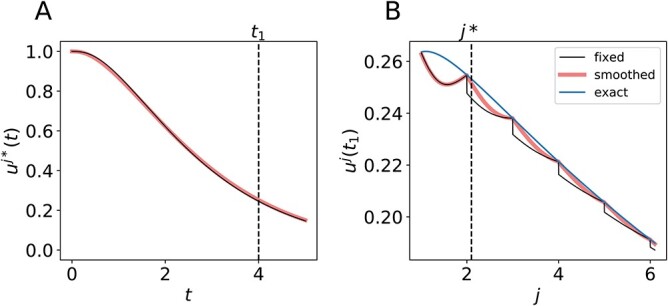
Trajectory dependence on the shape parameter is not smooth. (A) The trajectory and for calculated with the fixed (black) and smoothed (red) hypoexponential approximations in (3.6). The exact solution is not shown as it overlaps with the two curves. (B) The graph of with , using the fixed (black) and smoothed (red) parameterizations of the hypoexponential approximation, and the exact solution (blue).

3.5 Approximation error estimates

The natural phase space for distributed DDEs such as (1.1) or (3.3) is the space of exponentially weighted functions (Cassidy, 2021; Diekmann & Gyllenberg, 2012). In general, solutions evolving from the space of measurable functions remain integrable with respect to (Cassidy & Humphries, 2019; Hale, 1974).

Now, for the rate parameter of the gamma distribution given by , solutions of the gamma-distributed DDE will satisfy the growth bound in (1.2) with . Furthermore, solutions of linear gamma-distributed DDE (1.1) are of the form with . To illustrate the increased accuracy offered by the hypoexponential approximation, we use this linear case to derive explicit bounds for the approximation error induced by replacing the gamma distribution in (1.1) by an Erlang distribution as in (3.1) or by the hypoexponential approximation in (3.3). In both cases, we will express the approximation error as the difference of the MGFs evaluated at and we will see that the hypoexponential approximation has one fewer term than the Erlang approximation.

3.5.1 Erlang-distributed DDE

In the Erlang approximation described in Section 3.1, we approximated the convolution integral in the gamma-distributed DDE

where is the rate of the approximating Erlang distribution, and the Erlang-distributed DDE (3.1) is otherwise identical to (1.1). Thus, to compute the error induced by this approximation, we consider the difference between the convolution integrals where  

We immediately obtain

where the MGF of the gamma-distributed random variable is given by

and is the MGF of the Erlang distribution

Then,

(3.7)

Using the binomial theorem and the fact that the Erlang distribution is parameterized so that the first moment matches that of the gamma distribution, we can write the numerator in (3.7) as

Thus, the approximation error in the Erlang approximation case (see Section 3.1) is order . We see from the above analysis that if , then (3.7) is identically 0 and the approximation is exact.

3.5.2 Hypoexponential approximations

Turning to the two moment approximations derived in Theorems 3.1 and 3.2, we see that the approximation error induced by integrating with respect to the random variable   is given by

Then, we obtain

(3.8)

where is the MGF of the random variable and is given by

Then, we see

(3.9)

By recalling that and the fact that the first two moments agree, we use the binomial theorem to write the numerator in (3.9) as

Now, recalling that and , we have

Thus, as and are entirely determined by the mean and variance of the gamma distribution, we can write the error (3.8) as

where Accordingly, we see that the approximation error is order , or one order better than the Erlang-distributed DDE approximation. We also see that for as as in Section 3.2, so (3.9) is identically 0, and the approximation is exact.

3.6 On three moment matching

The ODE approximations in this section aim to replicate the gamma-distributed DDE by matching the first (in the case of the Erlang approximation) or first and second moments (in the hypoexponential approximations) of the underlying gamma distribution. It is natural to ask if a similar technique could allow for a more accurate approximation by matching the first three moments. To address this question, it is simpler and equivalent to match first three cumulants, rather than moments, of gamma and hypoexponential. The cumulant generating function of a gamma-distributed random variable with shape and rate parameters and is given by

Therefore, the cumulants are

Conversely, the cumulant generating function of hypoexponential-distributed random variable is given by

Therefore, the cumulants of are given by

Now, we show that if a hypoexponential distribution matches the first three cumulants, and thus moments, of then .

Theorem 3.3.

Let be a gamma-distributed random variable and assume that such that for . Then, .

Proof.

Without loss of generality by scaling, we take . Write , so that . The following system of equations for the first three cumulants must hold

Now, consider the sum . We have and therefore

As all terms of are non-negative, we must have for all . As , we obtain for all . It follows that and .

We therefore conclude that it is not possible to match the first three moments of a generic gamma distribution using a hypoexponential approximation. This three moment matching problem has been extensively studied (Bobbio et al., 2005; Osogami & Harchol-Balter, 2006). A generalized hypoexponential random variable corresponding to a Markov chain where each stage is visited at most once, i.e. the linear chain flows in one direction but some stages can be skipped, can be used to match the first three moments of gamma-distributed random variable. However, these generalized hypoexponential random variables are more demanding to implement than the hypoexponential approximations derived in Theorems 3.1 and 3.2. In short, their output varies depending on normalized moments, require at least as many parameters as the hypoexponential approximations, and the non-zero probability of skipping stages does not allow for a simple skip-free Markov chain interpretation as in the hypoexponential approximation.

4. Numerical results

Here, we illustrate the analytical results of Section 2 and evaluate the hypoexponential approximations derived in Section 3.2 by comparing the direct simulation of (1.1) using the FCRK method in Section 2 against the numerical simulation of the approximate ODE (3.3) and the Erlang distributed DDE (3.1). We first show that the FCRK method for (1.1) is accurate to the order demonstrated in Theorem 2.1. We then test the accuracy of the hypoexponential approximation derived in Section 3.2 using our FCRK method to provide reference solutions of generic gamma-distributed DDEs.

4.1 Numerical verification of the FCRK method

We test the fourth-order FCRK numerical solver by comparing the output of the FCRK method for (1.1) against differential equations with known, or reference, solutions. To obtain these known solutions, we first consider (1.1) in the case where the shape parameter is an integer. The gamma distribution in (1.1) is thus an Erlang distribution so, using the linear chain technique, we derive an equivalent ODE formulation. This equivalent ODE formulation can either be solved analytically or simulated using established techniques for systems of ODEs as implemented in Matlab to give the reference solution .

We simulate the Erlang-distributed DDE (1.1) using our fourth-order FCRK method to compute the numerical solution for a given step size . Then, to compute the accuracy of our simulation, we compute the error between the solution of (1.1), as obtained using our FCRK method, and the reference solution, obtained via the equivalent ODE. In general, when using a th order FCRK method, the error between the numerical solution, and the reference solution, , satisfies

where is the stepsize of the FCRK method. The error then satisfies

Therefore, we consider the error as a function of the step size of the FCRK method and thus compute for a various values of . The slope of as a function of is the order of the FCRK method.

4.1.1 Linear test problem

We first consider the linear test problem

(4.1)

where we set , and choose so the mean delay time . In this case, we can use the linear chain technique to reduce the Erlang distributed DDE in (4.1) to

(4.2)

where

Equation (4.2) is a linear system of ODEs and has an exact solution given by matrix exponentials. For , the analytical solution is

Thus, we simulate (4.1) using the fourth-order FCRK method described in the preceding section for and compare it against the analytic solution of (4.2) for on the interval . Furthermore, we simulate (4.1) for and . To compute reference solutions for , we use the fourth-order variable step size RK solver in Matlab (MATLAB, 2017) with an absolute and relative error tolerance of . We show the error on the log-log scale and the solution of the DDE in Figure 2.

Fig. 2.

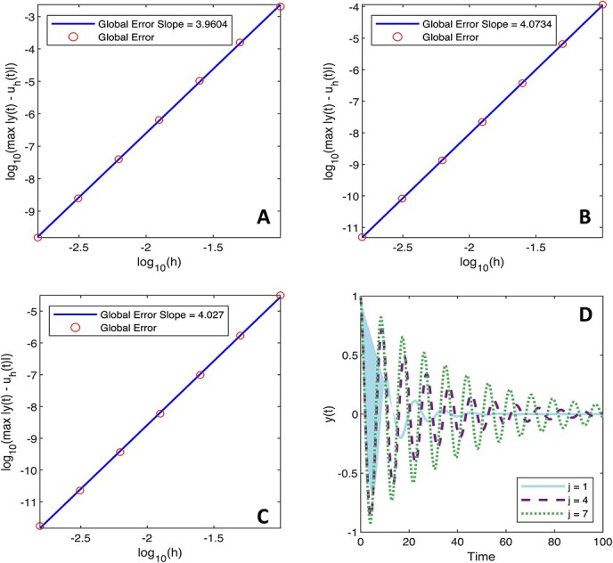
Convergence plots for the linear test problem (4.1). We plot as a function of . The slope of gives the convergence rate. is the simulation of (4.1) using the fourth-order FCRK method from Section 2 with fixed step size and is the solution of the equivalent ODE (4.2). Figure (A) shows the comparison against the exact solution when , while figures (B) and (C) show the error between and for and , respectively. Figure (D) shows the solution of the DDE for each test case. The solution of the equivalent ODE (4.2) is calculated using the fourth-order RK method RK45 in Matlab with relative and absolute error tolerance of .

4.1.2 Nonlinear test problem

We next consider the nonlinear test problem

(4.3)

where we set , take , and choose which gives . Once again, we set

and use the linear chain technique to reduce (4.3) to

(4.4)

Equation (4.4) is a nonlinear system of ODEs so we do not expect to find an analytical solution. Rather, we once again solve the system of ODEs (4.4) using the fourth-order variable step size RK solver in Matlab (MATLAB, 2017). We solve (4.4) with a tolerance of and compare this numerical solution against the numerical solution of (4.3) obtained using the FCRK method described in Section 2 on the interval . We show the error on the log-log scale for and and the solution of the DDE in Figure 3.

Fig. 3.

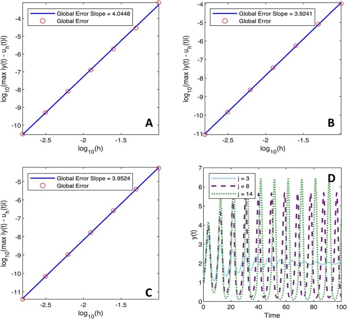
Convergence plots for the nonlinear test problem (4.3). We plot as a function of . The slope of gives the convergence rate. is the simulation of (4.3) using the fourth-order FCRK method from Section 2 with fixed step size and is the solution of the equivalent ODE (4.4). Panels (A—C) show the error between and for , respectively. Panel (D) shows the solution of the DDE for each test case. The solution of the equivalent ODE (4.4) is calculated using the fourth-order RK method RK45 in Matlab with relative and absolute error tolerance of .

4.1.3 Linear gamma-distributed DDE

Thus far, we have tested the FCRK method developed in section 2 by simulating Erlang-distributed DDEs and comparing the numerical solution against the solution of the equivalent ODE system. Here, we test our numerical method against a known solution of a gamma-distributed DDE with . In short, we consider

(4.5)

We note that is a solution (4.5) and make the ansatz . Inserting gives the characteristic function

where is the Laplace transform of the function evaluated at . It follows that for MGF of the gamma-distributed random variable evaluated at Thus, a solution of (4.5) must satisfy

(4.6)

which implies

Now, for simplicity, we set so that and

(4.7)

is a solution of the characteristic function where we must impose . The corresponding eigenfunction is the solution of the linear-distributed DDE for the history function We have thus determined an analytical solution to the linear gamma-distributed DDE (4.5) in against which we can compare the numerical solution obtained by the FCRK method.

Now, we consider parameter triples , set and calculate by taking the principal root in (4.7). In Fig. 4, we show the convergence of the numerical solution of (4.5) obtained using the FCRK method to the analytical solution for the parameter triples and on the interval .

Fig. 4.

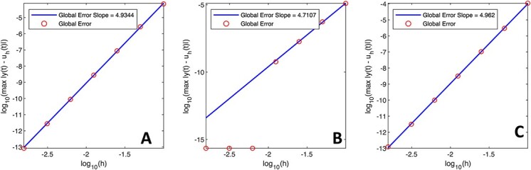
Convergence plots for the linear gamma-distributed DDE test problem (4.5). We plot as a function of where is the simulation of (4.5) using the fourth-order FCRK method from Section 2 and is the analytical solution of the linear-distributed DDE. In B, the error reaches machine precision for A–C show the error between and for the parameter triples given by and , respectively.

We note that for the DDEs (4.1) and (4.3), we observe the predicted convergence rate with approximate slope 4 until we reach numerical precision. For the DDE (4.5), the convergence rate is higher than expected and close to 5. However, the DDE (4.5) is linear and its solution is particularly simple being composed of a single exponential function. Numerical analysis is replete with examples of methods which exhibit a higher than required convergence order for certain problems, and this seems to just be another such example. We therefore conclude that the FCRK method derived in Section 2 exhibits the fourth-order global accuracy demonstrated in Theorem 2.1. These numerical tests, when combined with Theorem 2.1, indicate that we can use our FCRK method to provide reference solutions when comparing the Erlang and hypoexponential approximations.

4.2 Numerical evaluation of Erlang and hypoexponential approximations

Having confirmed the accuracy of our FCRK method to solve the distributed DDE (1.1), we now evaluate the Erlang and hypoexponential approximations for the two test problems (4.1) and (4.3) for . To test the accuracy of the Erlang approximation from Section 3.1, we use (3.2) with shape parameter and corresponding rate . We also consider the fixed hypoexponential approximation as described in Section 3.2 with and the rates and as given in Theorem 3.1. In these simulations, the fixed and smoothed approximations are indistinguishable, so we only show the fixed approximation corresponding to .

In the following simulations, we consider (4.1) and with , , and a non-constant history function given by for . We simulate the nonlinear test problem (4.3) for and with a constant history function .

In all cases shown in Fig. 5, the Erlang approximation has a visibly larger error than the hypoexponential approximations. In fact, there is no perceptible difference between the fixed (and consequently, the smoothed) hypoexponential approximation and the solution of the gamma-distributed DDE. While we only present the simulation results for a limited number of test problems, the significantly improved approximation by the hypoexponential approximation, compared against the Erlang approximation, was confirmed by a number of other test cases.

Fig. 5.

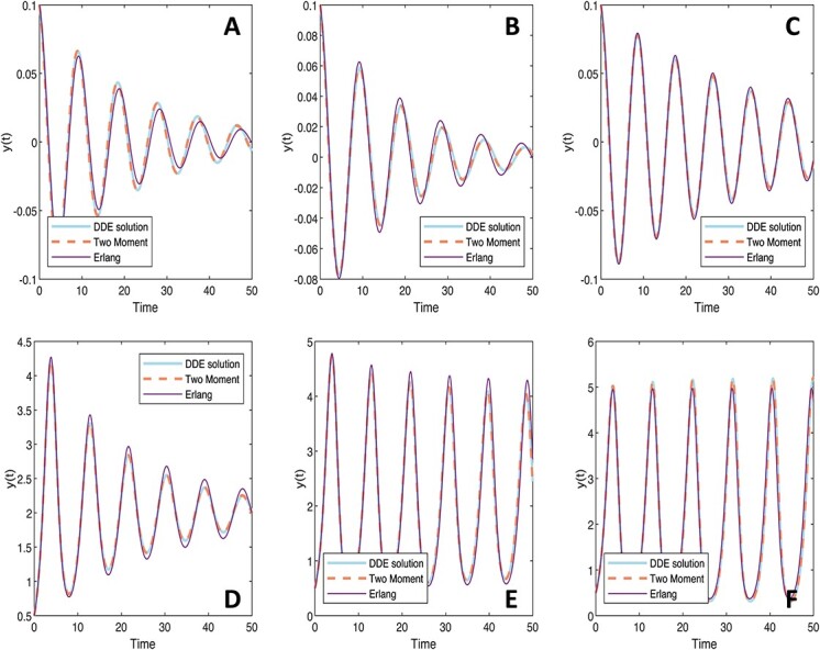
Comparison of ODE approximations to the gamma-distributed DDE (1.1) using the Erlang approximation in equation (3.2) or the fixed hypoexponential approximation in (3.5). In all cases, the solution of the gamma-distributed DDE as solved using the FCRK method is in solid blue, the solution of the fixed hypoexponential two moment approximation is in dashed orange and the solution of the Erlang approximation is in purple. A–C show the solution of the linear test problem (4.1) for and , respectively. D–F show the solution of the nonlinear test problem (4.3) for and , respectively.

4.2.1 Effects on linear stability

To study the effects of replacing the gamma-distributed DDE (1.1) by an Erlang or either hypoexponential approximation, we consider the linear gamma-distributed DDE given in (4.5). We note that is an equilibrium solution of the linear DDE, and it follows that this linear DDE represents the linearised version of

where and and . The principle of linearized stability for delay equations with infinite delay was established by Diekmann & Gyllenberg (2012) and, in short, indicates that the qualitative behaviour of a DDE with infinite delay near an equilibrium solution is determined by the linearized version of the DDE.

As a final test of the Erlang and hypoexponential approximations, we consider two specific examples with and parameters and and chosen near a bifurcation point. We identified the bifurcation point by following the same analysis as in Campbell & Jessop (2009) and Jessop & Campbell (2010) to calculate the region of stability of the equilibrium solution. There, the authors used as a solution ansatz for the linear DDE (4.5) and calculated conditions to ensure that the characteristic equation has a purely imaginary pair of roots.

In Fig. 6, we show that the hypoexponential approximation has the same stability properties as the solution of the distributed DDE, but that the Erlang approximation does not have the same stability properties. Essentially, for values of near the bifurcation point , the Erlang approximation requires rounding to the nearest integer, which may fall on the opposite side of the bifurcation point, so . Consequently, the Erlang approximation does not replicate the same qualitative behaviour as the gamma DDE. While we did not observe qualitative disagreement between the hypoexponential approximation and the gamma DDE in our simulations, it is possible for the hypoexponential approximation to fail in the same manner, although the Erlang approximation would also fail in this case. In Fig. 6A, we set and , while in Fig. 6B, we set and . We parameterize the Erlang and hypoexponential approximations as previously described in Sections 3.1 and 3.2.

Fig. 6.

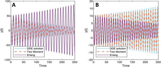
Comparison of ODE approximations to the gamma-distributed DDE (4.5) using the Erlang approximation in equation (3.2) or the fixed hypoexponential two moment approximation in (3.5) showing that the Erlang approximation does not have the same stability properties as the gamma-distributed DDE or the hypoexponential approximation. In all cases, the solution of the gamma-distributed DDE as solved using the FCRK method is in solid blue, the solution of the hypoexponential approximation is in dashed orange and the solution of the Erlang approximation is in purple.

These examples indicate that using an Erlang approximation to replace the gamma-distributed DDE can introduce extreme approximation error and may not replicate the qualitative behaviour of the original gamma distributed DDE. However, these simulations also indicate that the hypoexponential approximation faithfully replicates the dynamics of the linearized gamma-distributed DDE. In this sense, these results strongly advocate for the use of the hypoexponential approximation derived in Section 3.2 rather than the usual Erlang approximation when attempting to approximate the solution of a gamma-distributed DDE with an ODE approximation.

5. Statistical inference

One benefit of the hypoexponential approximation of a gamma-distributed DDE is that it is easily implemented in existing inference software. Here, we demonstrate a possible implementation, using the simple and ubiquitous example of the Kermack–McKendrick (SIR) model from epidemiology, and the probabilistic programming language Stan (Carpenter et al., 2017). For this example, we deliberately choose a simplistic scenario, but the same ideas can be used for more realistic models. We first show how one can formulate the SIR model as a system of DDEs. Then, we derive the hypoexponential ODE approximation using the machinery developed above. We then show how one can build a simple statistical model for two independent data streams that both inform the model’s parameters (including the shape parameter ). Finally, we fit the model to simulated data.

5.1 The Kermack–McKendrik model as a system of DDEs

The SIR model describes fractions of susceptible (), infected () and recovered () individuals in a population affected by a pathogen. In our version, the duration of the infectious period is distributed. Hence, in this example, we ignore individuals that were exposed to the pathogen, but not yet infectious. The mean duration of the infectious period is and the variance is . The infection rate and the initial fraction infected in the population are denoted and , respectively. The model is then given by the following system of DDEs:

(5.1)

The variable represents the instantaneous incidence, which is equal to for , and we define for to jump-start the epidemic (Champredon et al., 2018). Here, is the Dirac delta measure at . In addition, when , we set and . Notice that and have a discontinuity at , and , and .

To understand why the system of DDEs (5.1) is correct, first notice that the equation for is the same as in the standard ODE SIR model: susceptible individuals are depleted at a rate equal to the incidence , assuming mass action. The equation for is a bit less intuitive. The first term represents influx of recently infected susceptible individuals, and the second term is a convolution integral of the same time-delayed incidence, and the PDF of . Hence, this convolution term represents the recovery of individuals at time that were infected time units ago, with the likelihood of recovery time units from infection given by .

A more formal way to derive (5.1) is to start with the renewal equation formulation of the Kermack–McKendrick model (see, e.g. Diekmann et al. (2012))

(5.2)

where is the survival function of the gamma distribution. The fraction of infectious individuals at time is then given by , an integral over all individuals infected at time that are still infectious at time . In order to derive DDE (5.1), we differentiate as follows:

Here, differentiating under the integral sign is justified as is bounded (for ) and bounded functions are integrable with respect to the measure on the interval .

5.2 The hypoexponential approximation of the DDE SIR model

We now approximate DDE (5.1) with a system of ODEs using the method developed in Section 3.2.

Lemma 5.1.

Using the hypoexponential approximation, the above DDE model (5.1) can be replaced by the following system of ODEs:

(5.3)

where we write , with and the rates are given by

(5.4)

As initial condition, we take , , and for .

Proof.

We first approximate the gamma distribution with the hypoexponential distribution with parameters and then use the linear chain trick to approximate the convolution integral . This results in the following system of ODEs:

(5.5)

The initial conditions for the auxiliary variables are given by

which holds because only if . Notice that and . Hence, for , and the equation for in system (5.5) is redundant.

5.3 A statistical model for epidemiological data

Reporting of incidence often happens at discrete time points , and the reported quantity is the accumulated number of cases observed between consecutive reporting times. Using the above model (5.1), we therefore use the cumulative incidence to simulate cases

(5.6)

where is a large (known) constant representing the catchment population size, and are (positive) reporting times, and we take . The simulated incidence data are shown in Fig. 7A. Conversely, given predictions of the model , we can compute the likelihood of data , using the probability mass function of the Poisson distribution.

Fig. 7.

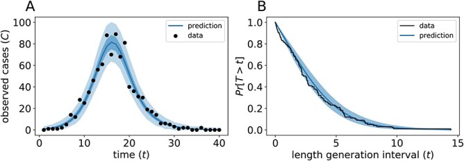
Simulated epidemic data and posterior predictive checks. (A) Simulated data and the model prediction . The dark-blue band represents the credible interval, and the light-blue band the prediction interval. (B) Simulated serial intervals represented as a empirical survival function (black), and the fitted survival function for given by (blue).

In addition to time series of the number of reported cases, often other data are collected to inform an epidemic model. For example, symptom onset data from transmission couples might be available. Such data consists of the times of symptom onset of pairs of individuals A and B, for whom it is known that A infected B (e.g. by means of genetic evidence). Transmission couple data give information about the length of the generation interval , which is defined as follows:

Definition 5.1.

Sample a random infected individual A from the population. Suppose that A was infected at time by individual B, and suppose that B was infected at time . The generation interval is then defined as

(5.7)

hence, the time between infection of individuals A and B.

Notice that different definitions of exist in the literature; we refer to Svensson (2007) for a discussion. In practice, the generation interval will almost never be observed but can be approximated by the serial interval, which is the time between symptom onset of individuals A and B.

Assuming that the duration of the infection is gamma distributed, the hypoexponential approximation method allows one to estimate the shape parameter of this distribution using both time series data and transmission couple data simultaneously, i.e. using ‘evidence synthesis’. For this, we still need a likelihood function for the transmission couple data.

Lemma 5.2.

As before, suppose that the length of the infectious period has a gamma distribution . The PDF of is given by

where is the (upper) incomplete gamma function.

Proof.

Here, we present only a sketch of the proof. See Svensson (2007) and references therein for more details. Let denote the PDF of . As in Definition 5.1, consider a randomly sampled individual A, infected at time and consider all individuals infected at time . Each of these individuals had an equal chance of infecting A, as long as they are still infectious at time , which is true with probability

(5.8)

Therefore, the probability density must be proportional to . To get a proper PDF, we must find the normalizing constant

(5.9)

Hence, we find that

(5.10)

which proves the lemma.

Suppose that we have observed serial intervals. Assuming for simplicity that symptom onset is immediate, the distribution of the serial interval and generation interval are identical. The log-likelihood of the data is now the sum of the log-likelihood of the case data , and the log-likelihood of the transmission-couple data , given parameters , is

(5.11)

where is the probability mass function of the Poisson distribution. To demonstrate this approach, we simulated, in addition to observed cases , a small number of generation times . The simulated serial interval data are shown in Fig. 7B.

We then used Stan to fit the model defined by (5.11) to the simulated data in a Bayesian framework, using improper flat priors for all parameters. In the Stan implementation, the DDE model (5.1) was replaced by the system of ODEs (5.3). The fitted model predictions are shown together with the simulated data in Fig. 7A and B. The marginal and joint posterior densities of the model parameters are shown in Fig. 8, together with the ground-truth values used to simulate the data. For all parameters, the ground-truth values are close to the modes of the marginal posterior distributions. We do find strong correlations between all pairs of parameters indicating practical identifiability issues.

Fig. 8.

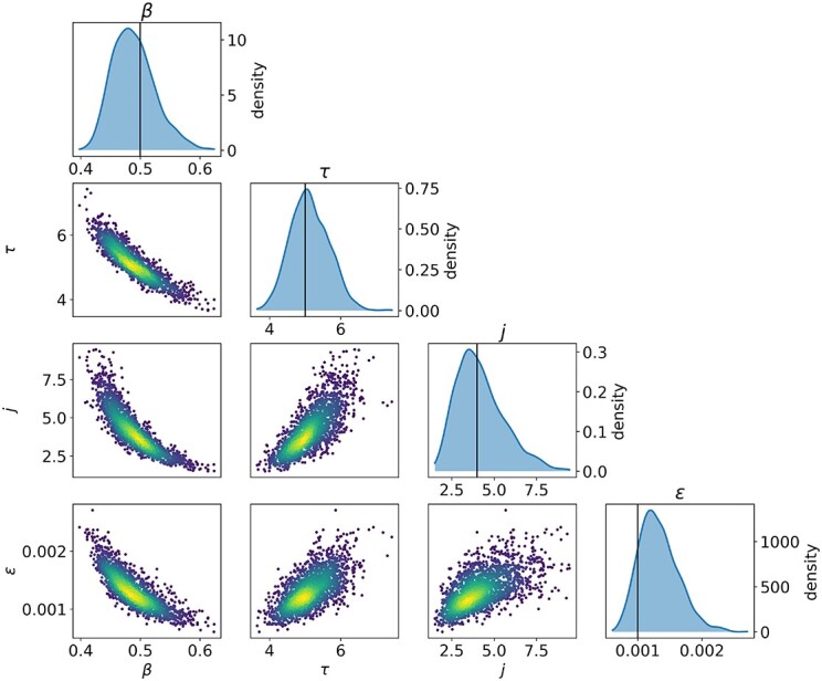
Posterior marginal and joint density for the epidemic model parameters. Each dot in the joint density scatter plots represents a Monte-Carlo sample from the posterior distribution. The color of the dots indicates the density. The black vertical lines represent the ground-truth parameter values. The ground-truth parameters used for the simulation are , , , , and .

In the SIR model, the shape parameter of the infectious period is hard to identify due to the correlation with other parameters, as shown in Fig. 8. Further complicating matters, the trajectories of the model as a function of are very similar when is large, which makes the likelihood of the incidence data not well behaved. This problem has also been described for in-vitro SHIV data (Beauchemin et al., 2017). To resolve such identifiability issues, it can be important to use other data to inform the parameter . In this example, we used synthetic serial intervals that could be observed during real-life epidemics using transmission pairs. The distribution of these serial intervals depends on the real-valued parameter . Therefore, to fit the model to both incidence data and serial intervals in an evidence synthesis framework, it is essential that the likelihood of the incidence data also depends on a real-valued shape parameter .

Furthermore, treating as a first-class real-valued parameter in a statistical model can be important for accurately and efficiently estimating important quantities as the basic reproduction number . For certain childhood diseases, the dynamics of an epidemiological model depend on is of a more qualitative nature (Krylova & Earn, 2013) due to bifurcations. As we have shown in Fig. 6, using an Erlang instead of the hypoexponential approximation in such cases can result in large deviations from the true gamma-distributed model.

The Stan model code and a python script to simulate data and fit the model are available on https://github.com/lanl/gamma-dde.

6. Discussion

Gamma-distributed DDEs, such as (1.1), occur throughout mathematical biology. However, modellers often make simplifying assumptions due to the lack of appropriate numerical methods for infinite delay models. In this work, we developed an FCRK method to numerically simulate gamma-distributed DDEs, established order conditions on the numerical quadrature technique to ensure the accuracy of the method, proved the convergence of the FCRK method and illustrated our results with a series of test problems. Despite the development of an FCRK method to simulate (1.1) in this work, many software packages rely on ODE solvers to perform parameter fitting and statistical inference. Accordingly, we derived a finite dimensional approximation of the gamma-distributed DDE using a hypoexponential approximation and used numerical simulation to show that this hypoexponential approximation outperforms the common Erlang approximation. In particular, we demonstrated that using the Erlang approximation can lead to qualitatively different behaviour than the hypoexponential approximation and the true solution of the gamma-distributed DDE. Finally, we implemented our finite dimensional approximation in Stan (Carpenter et al., 2017) to fit synthetic data from a hypothetical epidemic.

The primary impediment towards the adaptation of FCRK methods to distributed DDEs with infinite delay is the accurate and consistent evaluation of the convolution integral (2.8). Here, we developed a change of variable that transforms the semi-infinite domain of integration to This change of variables is parametrized by certain parameters and , and we give conditions on and to ensure that the transformed integrand is sufficiently smooth to implement standard quadrature rules in Lemma 2.1. These conditions, and thus the change of variable and FCRK method, apply to other delay distributions that decay exponentially. Accordingly, the FCRK method framework developed in this article should extend with minimal changes to other distributed DDEs with infinite delays.

Until such FCRK methods are implemented in common software packages such as Stan, it is useful to have accurate finite dimensional approximations of the distributed DDE (1.1). Many finite dimensional approximations have been developed recently. The hypoexponential approximation described in Section 3 offers a number of advantages over existing methods. While our analysis of the approximation error does not allow for an explicit expression of the error introduced by replacing the gamma distribution by either the Erlang or hypoexponential distribution, the calculation in Section 4.2 offers a heuristic explanation for why the hypoexponential distribution is more accurate than the common Erlang approximation. As our numerical simulations show, there are gamma-distributed DDE problems for which the hypoexponential method gives the correct qualitative behaviour, while the Erlang approximation exhibits incorrect asymptotic stability behaviour. Moreover, unlike existing algorithms to parametrize phase-type distributions that do not give explicit values for the parameters of the phase-type distribution, we explicitly derived the parameters of the hypoexponential distribution as a function of the mean and variance of the underlying gamma distribution. This explicit expression for the rates allows for simple implementation in software packages such as Stan and we showed how to implement a simple SIR model with a gamma-distributed duration of infection. This example explicitly showed how the hypoexponential approximation derived in Section 3 facilitates evidence synthesis that is necessary to identify important model parameters.

Our work represents a step towards relaxing the assumption of Erlang-distributed delays in, amongst many other applications, infectious disease epidemiology. The FCRK method developed in this work allows modellers to directly simulate a gamma-distributed DDE if precise numerical results are necessary, while the hypoexponential approximations offer a more accurate ODE representation of the underlying DDE than the common Erlang approximation without any increase in complexity. Accordingly, we have presented two distinct pathways to allow for the implementation of gamma-distributed DDEs and facilitate their use in mathematical biology or other fields of science.

A. Smoothness conditions for the FCRK method

In the main text, we derived sufficient conditions on the change of variable

to ensure that the transformed convolution integral is sufficiently smooth to not introduce unnecessary error in the FCRK method. Here, we prove that these conditions are sufficient by giving the proof of Lemma 2.1.

We recall that is the solution of the gamma-distributed DDE and is the PDF of the gamma distribution with shape parameter and rate parameter , and we are calculating

We first show that the derivatives of with respect to can be computed inductively.

Lemma A.1.

Assume that is times differentiable and take . Then,

where is a constant depending only on , and is an integer between and , inclusive.

Proof.

The proof is by induction on the order of the derivative . The case follows immediately from the definition of , while the st case comes from term by term differentiation with

We now must show that is a bounded function of on . Take and consider the compact interval away from , We note that is a product of continuous functions, and thus continuous, so the image of this compact set is compact and thus bounded. Then, we consider the interval and define

for . We note that, for and , appears in the derivative of . Now, for and we compute

Thus, for sufficiently close to and , we have and we can therefore bound from above as

Now, we multiply by so

Then, as we have Recalling that the weight parameter of the function space satisfies , we set and thus obtain

Then, as we immediately see

so is bounded and it follows from the definition of the space that

for all . We thus conclude that

It follows that and thus the integrand is bounded on the entire interval The condition is crucial in the above calculation, as it implies that and leads to the result.

Lemma A.2.

Assume that is times differentiable and set

(A1)

Then, is times differentiable in for . Furthermore, if the th derivative of , , is bounded for , then there exists such that

for .

Proof.

We recall that so taking ensures that and The bound of follows from the boundedness of demonstrated previously.

B. The smoothed hypoexponential approximation

Here, we give the proof of Theorem 3.2 that established the rates of smoothed hypoexponential approximation. As in the main text, let denote the mean of a gamma-distributed random variable , and let denote the shape parameter, such that has variance . We write for the rate parameter, and for the smallest integer greater than . We recall the definition of the smoothed hypoexponentially distributed random variable with the same mean and variance as

Theorem B.1.

Let be a -distributed random variable where Consider the hypoexponentially distributed random variable with rate parameters . Recall that as , set and define and by

(B1)

Then, and have the same first two moments.

Proof. Proof of Theorem B.1 —

The mean of and are given by and

because the square-roots in Eq (B1) cancel. Now using the fact that , we indeed find that . The variance of is equal to and the variance of is given by

For any two numbers and , we have . Hence, we find that

Therefore, , which proves the theorem.

Remark B.1.

Notice that the values and are the roots of the quadratic polynomial

C. Convergence of the FCRK Method

Here, we demonstrate the convergence of the FCRK method described in Section 2 and prove Theorem 2.1. In the following analysis, we make extensive use of the results in Section 6 of Maset et al. (2005) and Section 7 of Bellen et al. (2009). We will also require the definitions of discrete and uniform order for FCRK methods (found in Definitions 2.3 and 2.2, respectively, and Definition 4.1 of Maset et al. (2005)).

To begin the analysis of our FCRK method, we transform the IVP (2.7) to an equivalent formulation that is simpler to analyse. In particular, we recall that, for all times ,

and is a continuous function of in the interval . We therefore define

The function is therefore a uniformly continuous function of and agrees with almost-everywhere in Therefore,

and we can consider the transformed problem

(C1)

Now, we do not calculate the right-hand side of (C1) precisely but rather use a quadrature rule to approximate the integral as discussed in the main text. Maset et al. (2005) considered FCRK methods for the generalized setting of all such approximations of the right-hand side of (C1). Maset et al. (2005) denoted approximations of the right-hand side of (C1) with a tilde which, in our setting, gives

where is a parameter that controls the precision of the approximation. Here, represents the space of composite quadrature rules with a fixed number of steps. These quadrature rules are defined by their weights, , and collocation points, . The quadrature rule is therefore represented by with

where and are the the step size and order of the quadrature method, respectively. Accordingly, the approximation of the right-hand side of (C1) is given by

(C2)

For notational simplicity in the following, we denote, for a given function ,

The accuracy of the approximation for a given function and quadrature rule is given by

(C3)

Maset et al. (2005) derived conditions on the approximation that permit convergence of existing FCRK methods. To establish the convergence of the FCRK method for the transformed problem (C1), the approximate function must satisfy the following conditions:

• (1) is uniformly continuous with respect to and the derivative with respect to the function , is continuous with respect to and uniformly bounded with respect to ;
• (2) There exists a continuous function such that for all and ;
• (3) is of class with respect to for all and both the derivatives are bounded uniformly with respect to

Furthermore, let be the largest value such that the IVP (1.1) has a unique solution with initial data over the interval . Denote the simulation mesh by

with corresponding step size . Finally, let the approximation of the solution obtained using a FCRK method with mesh given by . Then, recalling the definitions of uniform, discrete and global Order in Definitions 2.2–2.4, Maset et al. (2005) prove.

Theorem C.1. Theorem 6.1 of Maset et al. (2005) —

If an FCRK method of uniform order , discrete order , with , and such that , is applied to (C1) for the computation of through and the following assumptions hold:

• A: for and for all with ;
• B:Conditions (1), (2) and (3) hold;
• C:The approximation error (C3) satisfies ;
• D: is 5 times continuously differentiable;

then for a fixed , and simulation meshes that include all possible discontinuity points of in . Then,

We note the relationship between the smoothness required of the solution and the maximal discrete and uniform orders for the FCRK method.

C.1 Applying Theorem (C.1) to the FCRK method

We now show that Theorem C.1 is applicable to the FCRK method derived in Section 2. Bellen et al. (2009) show that the global fourth-order explicit method considered in this work has uniform order 3 and discrete order 4 and simple inspection shows that (2.4) satisfies Assumption A. Next, we show that our approximation satisfies the conditions (1), (2) and (3) and so verify Assumption B.

In what follows, we consider arbitrary functions Furthermore, we only consider quadrature rules with bounded weights

(C4)

for fixed . Finally, we assume that the function is at least times continuously differentiable and globally Lipschitz. The solution is thus times differentiable for . Thus, Assumption D is satisfied. Furthermore, we assume that and are bounded for .

C.1.1 Verifying condition (1)

We begin with condition (1). Now, is Lipschitz and thus uniformly continuous. Therefore, for each there exists such that for all , . Then, it follows from the definition (C2), the uniform continuity of with respect to is equivalent to showing that we can choose such that if the quadrature rules satisfy then the quadrature method is such that

This relationship, combined with the uniform continuity of , will establish the uniform continuity of with respect to . We now show how to choose such a By adding 0 to the above expression, we obtain

Now, is uniformly continuous and the the sum of the weights is bounded above by . From the uniform continuity of , we can choose , independently of and , such that if , so that then

Therefore, we obtain

Furthermore, is the product of bounded functions and thus bounded above. Let this upper bound be given by and note that it is independent of the quadrature rule used. Accordingly, it is possible to constrain so that the weights of the quadrature rule satisfy

It thus follows that

Therefore, independently of the quadrature rule , taking

is sufficient to ensure that

As was chosen from the uniform continuity of the function , it thus follows that is uniformly continuous in as desired.

Furthermore, is continuously differentiable and the mapping

is linear, and thus differentiable with respect to The chain rule for Fréchet derivatives gives

which is continuous with respect to and bounded with respect to by virtue of the bound on the quadrature weights (C4). The condition (1) is therefore satisfied.

C.1.2 Verifying condition (2)

We turn now to the second condition. From the definition of we immediately see that

where is the step size of the th order quadrature method and is a known error term from the Taylor expansion of . Recalling that is assumed to be bounded, we obtain

which gives

It is clear that is a continuous function and satisfies condition (2).

C.1.3 Verifying condition (3)

It remains to show that is with respect to for all Now, is 4 times continuously differentiable and is linear in Therefore, consecutive applications of the chain rule for Fréchet derivatives gives the required regularity of . Furthermore, the quadrature weights satisfy (C4) and we have assumed that for is bounded. Therefore, Lemma A.2 yields the uniform boundedness of for with respect to , as required.

C.1.4 Characterization of the accuracy of the approximation of

We now consider the approximation error defined in (C3) and show that Assumption C holds. To calculate in the FCRK method defined in Section 2, we considered composite quadrature rules of order with maximal step-size . Such quadrature rules satisfy

Then, Taylor expanding the latter expression in (C2) gives

The boundedness of gives In Section 2, we chose such that . It follows that the FCRK method (2.4) satisfies Assumption C.

C.2 A convergence result for the FCRK method

Assumption A of Theorem C.1 is satisfied for the the fourth-order explicit FCRK method defined in (2.4) with uniform order and discrete order . We have shown that both Assumptions B and C hold, while the assumption that is 4 times continuously differentiable ensures that Assumption D holds. We thus conclude

Theorem C.2.

Assume that the right-hand side of (1.1) is 4 times continuously differentiable and let be the explicit FCRK method with global fourth-order defined in (2.4). Furthermore, let the simulation mesh include all breaking points of the DDE (1.1) and have maximal stepsize . Let the quadrature method be given by the composite Simpson’s open rule with maximal sub-interval size of .

Then, the error between the solution, of (1.1) and the numerical approximation of the solution, , satisfies

Funding

National Institutes of Health (R01-OD011095 supported C.H.v.D., T.C., R01-AI116868 supported T.C.); National Science and Engineering Research Council of Canada (RGPIN-2018-05062 to A.R.H.); National Science and Engineering Research Council Undergraduate Student Research Award to P.G. US Department of Energy (contract no. 89233218CBA000001) supported C.H.v.D and T.C..

Bibliography

- Andò, A., Breda, D. & Gava, G. (2020) How fast is the linear chain trick? A rigorous analysis in the context of behavioral epidemiology. Math. Biosci. Eng., 17, 5059–5084. [DOI] [PubMed] [Google Scholar]
- Beauchemin, C. A., Miura, T. & Iwami, S. (2017) Duration of SHIV production by infected cells is not exponentially distributed: Implications for estimates of infection parameters and antiviral efficacy. Sci. Rep., 7, 42765. 10.1038/srep42765. [DOI] [PMC free article] [PubMed] [Google Scholar]
- Bellen, A., Maset, S., Zennaro, M. & Guglielmi, N. (2009) Recent Trends in the Numerical Solution of Retarded Functional Differential Equations. Acta Numerica, 18, 1–110. [Google Scholar]
- Bellen, A. & Zennaro, M. (2013) Numerical Methods for Delay Differential Equations, 1st edn. Oxford: Oxford University Press. [Google Scholar]
- Bobbio, A., Horváth, A. & Telek, M. (2005) Matching three moments with minimal acyclic phase type distributions. Stoch. Model., 21, 303–326. [Google Scholar]
- Breda, D., Diekmann, O., Gyllenberg, M., Scarabel, F. & Vermiglio, R. (2016) Pseudospectral discretization of nonlinear delay equations: new prospects for numerical bifurcation analysis. SIAM J. Appl. Dyn. Syst., 15, 1–23. [Google Scholar]
- Câmara De Souza, D., Craig, M., Cassidy, T., Li, J., Nekka, F., Bélair, J. & Humphries, A. R. (2018) Transit and lifespan in neutrophil production: implications for drug intervention. J. Pharmacokinet. Pharmacodyn., 45, 59–77. [DOI] [PubMed] [Google Scholar]
- Campbell, S. A. & Jessop, R. (2009) Approximating the Stability Region for a Differential Equation with a Distributed Delay. Math. Model. Nat. Phenom., 4, 1–27. [Google Scholar]
- Carpenter, B., Gelman, A., Hoffman, M., Lee, D., Goodrich, B., Betancourt, M., Brubaker, M., Guo, J., Li, P. & Riddell, A. (2017) Stan: a probabilistic programming language. J. Stat. Softw., 76, 1–32. [DOI] [PMC free article] [PubMed] [Google Scholar]
- Cassidy, T. (2021) Distributed delay differential equation representations of cyclic differential equations. SIAM J. Appl. Math., 81, 1742–1766. [Google Scholar]
- Cassidy, T. & Craig, M. (2019) Determinants of combination GM-CSF immunotherapy and oncolytic virotherapy success identified through in silico treatment personalization. PLOS Comput. Biol., 15, e1007495. [DOI] [PMC free article] [PubMed] [Google Scholar]
- Cassidy, T., Craig, M. & Humphries, A. R. (2019) Equivalences between age structured models and state dependent distributed delay differential equations. Math. Biosci. Eng., 16, 5419–5450. [DOI] [PubMed] [Google Scholar]
- Cassidy, T. & Humphries, A. R. (2019) A mathematical model of viral oncology as an immuno-oncology instigator. Math. Med. Biol. A J. IMA, 37, 117–151. [DOI] [PubMed] [Google Scholar]
- Champredon, D., Dushoff, J. & Earn, D. J. D. (2018) Equivalence of the Erlang-distributed SEIR epidemic model and the renewal equation. SIAM J. Appl. Math., 78, 3258–3278. [Google Scholar]
- Cryer, C. W. & Tavernini, L. (1972) The numerical solution of Volterra functional differential equations by Euler’s method. SIAM J. Numer. Anal., 9, 105–129. [Google Scholar]
- Diekmann, O. & Gyllenberg, M. (2012) Equations with infinite delay: blending the abstract and the concrete. J. Differ. Equ., 252, 819–851. [Google Scholar]
- Diekmann, O., Gyllenberg, M. & Metz, J. A. J. (2018) Finite dimensional state representation of linear and nonlinear delay systems. J. Dyn. Differ. Equations, 30, 1439–1467. [Google Scholar]
- Diekmann, O., Gyllenberg, M. & Metz, J. A. J. (2020a) Finite dimensional state representation of physiologically structured populations. J. Math. Biol., 80, 205–273. [DOI] [PMC free article] [PubMed] [Google Scholar]
- Diekmann, O., Heesterbeek, H. & Britton, T. (2012) Mathematical Tools for Understanding Infectious Disease Dynamics. Princeton University Press. [Google Scholar]
- Diekmann, O., Scarabel, F. & Vermiglio, R. (2020b) Pseudospectral discretization of delay differential equations in sun-star formulation: Results and conjectures. Discret. Contin. Dyn. Syst. - S, 13, 2575–2602. [Google Scholar]
- Enright, W. H. and Hayashi, H. (1997). A delay differential equation solver based on a continuous Runge-Kutta method with defect control. Numer. Algorithms, 16(3–4):349. [Google Scholar]
- Eremin, A. (2016) Functional continuous Runge-Kutta-Nyström methods. Electron. J. Qual. Theory Differ. Equ., Proc. 10'th Coll. Qualitative Theory of Diff. Equ. (July 1–4, 2015, Szeged, Hungary) Ed. by T. Krisztin. SZTE: Szeged. Bolyai Institute, No. 11, pp. 1–17. 10.14232/ejqtde.2016.8.11. [DOI] [Google Scholar]
- Eremin, A. S. (2019) Runge-Kutta methods for differential equations with distributed delays. AIP Conf. Proc, vol. 2116, p. 140003. [Google Scholar]
- Eremin, A. S., Humphries, A. R. & Lobaskin, A. A. (2020) Some issues with the numerical treatment of delay differential equations. Int. Conf. Numer. Anal. Appl. Math. Icnaam 2019, vol. 2293, p. 100003. [Google Scholar]
- Gossel, G., Hogan, T., Cownden, D., Seddon, B. & Yates, A. J. (2017) Memory CD4 T cell subsets are kinetically heterogeneous and replenished from naive T cells at high levels. Elife, 6, 1–30. [DOI] [PMC free article] [PubMed] [Google Scholar]
- Greenhalgh, S. & Rozins, C. (2021) A generalized differential equation compartmental model of infectious disease transmission. Infect Dis Model, 6, 1073–1091. [DOI] [PMC free article] [PubMed] [Google Scholar]
- Gyllenberg, M., Scarabel, F. & Vermiglio, R. (2018) Equations with infinite delay: Numerical bifurcation analysis via pseudospectral discretization. Appl. Math. Comput., 333, 490–505. [Google Scholar]
- Hale, J. K. (1974) Functional differential equations with infinite delays. J. Math. Anal. Appl., 48, 276–283. [Google Scholar]
- Hale, J. K. & Verduyn Lunel, S. M. (1993) Introduction to Functional Differential Equations. Applied Mathematical Sciences (F. John, J.E. Marsden & L. Sirovich eds), vol. 99. New York, NY: Springer. [Google Scholar]
- Hino, Y., Murakami, S. & Naito, T. (1991) Functional Differential Equations with Infinite Delay. Lecture Notes in Mathematics (A Dold, B. Eckmann & F. Takens eds), vol. 1473. Berlin Heidelberg, Berlin, Heidelberg: Springer. [Google Scholar]
- Hu, S., Dunlavey, M., Guzy, S. & Teuscher, N. (2018) A distributed delay approach for modeling delayed outcomes in pharmacokinetics and pharmacodynamics studies. J. Pharmacokinet. Pharmacodyn., 45, 1–24. [DOI] [PubMed] [Google Scholar]
- Hurtado, P. & Richards, C. (2020) Time is of the essence: incorporating phase-type distributed delays and dwell times into ODE models. Math. Appl. Sci. Eng., 1, 410–422. [Google Scholar]
- Hurtado, P. J. & Kirosingh, A. S. (2019) Generalizations of the ‘Linear Chain Trick’: incorporating more flexible dwell time distributions into mean field ODE models. J. Math. Biol., 79, 1831–1883. [DOI] [PMC free article] [PubMed] [Google Scholar]
- Jenner, A. L., Cassidy, T., Belaid, K., Bourgeois-Daigneault, M.-C. & Craig, M. (2021) In silico trials predict that combination strategies for enhancing vesicular stomatitis oncolytic virus are determined by tumor aggressivity. J. Immunother. Cancer, 9, e001387. [DOI] [PMC free article] [PubMed] [Google Scholar]
- Jessop, R. & Campbell, S. (2010) Approximating the stability region of a neural network with a general distribution of delays. Neural Networks, 23, 1187–1201. [DOI] [PubMed] [Google Scholar]
- Johnson, M. A. & Taaffe, M. R. (1989) Matching moments to phase distributions: mixtures of erlang distributions of common order. Commun. Stat. Stoch. Model., 5, 711–743. [Google Scholar]
- Johnson, M. A. & Taaffe, M. R. (1990) Matching moments to phase distributions: density function shapes. Commun. Stat. Stoch. Model., 6, 283–306. [Google Scholar]
- Koch, G. & Schropp, J. (2015) Distributed transit compartments for arbitrary lifespan distributions in aging populations. J. Theor. Biol., 380, 550–558. [DOI] [PubMed] [Google Scholar]
- Krylova, O. & Earn, D. J. (2013) Effects of the infectious period distribution on predicted transitions in childhood disease dynamics. J R Soc Interface, 10, 20130098. [DOI] [PMC free article] [PubMed] [Google Scholar]
- Krzyzanski, W. (2019) Ordinary differential equation approximation of gamma distributed delay model. J. Pharmacokinet. Pharmacodyn., 46, 53–63. [DOI] [PubMed] [Google Scholar]
- Langlois, G. P., Craig, M., Humphries, A. R., Mackey, M. C., Mahaffy, J. M., Bélair, J., Moulin, T., Sinclair, S. R. & Wang, L. (2017) Normal and pathological dynamics of platelets in humans. J. Math. Biol., 75, 1411–1462. [DOI] [PubMed] [Google Scholar]
- Lixoft (2019) Monolix version 2019R2. Lixoft SAS: Antony; France. http://lixoft.com/products/monolix. [Google Scholar]
- MacDonald, N. (1978) Time Lags in Biological Models, 1st edn. Berlin: Springer. [Google Scholar]
- Maset, S., Torelli, L. & Vermiglio, R. (2005) Runge-Kutta Methods for Retarded Functional Differential Equations. Math. Model. Methods Appl. Sci., 15, 1203–1251. [Google Scholar]
- MATLAB (2017) R2017a. Natick, MA: The MathWorks Inc. [Google Scholar]
- Osogami, T. & Harchol-Balter, M. (2006) Closed form solutions for mapping general distributions to quasi-minimal PH distributions. Perform. Eval., 63, 524–552. [Google Scholar]
- Raue, A., Karlsson, J., Saccomani, M. P., Jirstrand, M. & Timmer, J. (2014) Comparison of approaches for parameter identifiability analysis of biological systems. Bioinformatics, 30, 1440–1448. [DOI] [PubMed] [Google Scholar]
- Raue, A., Kreutz, C., Maiwald, T., Bachmann, J., Schilling, M., Klingmüller, U. & Timmer, J. (2009) Structural and practical identifiability analysis of partially observed dynamical models by exploiting the profile likelihood. Bioinformatics, 25, 1923–1929. [DOI] [PubMed] [Google Scholar]
- Roberts, M. G. & Heesterbeek, J. A. (2007) Model-consistent estimation of the basic reproduction number from the incidence of an emerging infection. J. Math. Biol., 55, 803–816. [DOI] [PMC free article] [PubMed] [Google Scholar]
- Rozhnova, G., van Dorp, C. H., Bruijning-Verhagen, P., Bootsma, M. C. J., van de Wijgert, J. H. H. M., Bonten, M. J. M. & Kretzschmar, M. E. (2021) Model-based evaluation of school- and non-school-related measures to control the covid-19 pandemic. Nat. Commun., 12, 1614. [DOI] [PMC free article] [PubMed] [Google Scholar]
- Sanche, S., Lin, Y. T., Xu, C., Romero-Severson, E., Hengartner, N. & Ke, R. (2020) High contagiousness and rapid spread of severe acute respiratory syndrome coronavirus 2. Emerg. Infect. Dis., 26, 1470–1477. [DOI] [PMC free article] [PubMed] [Google Scholar]
- Smith, H. (2011) An introduction to delay differential equations with applications to the life sciences. Texts in Applied Mathematics (J.E. Marsden, L. Sirovich & S.S. Antman eds), vol. 57. New York, NY: Springer. [Google Scholar]
- Svensson, Å. (2007) A note on generation times in epidemic models. Math. Biosci., 208, 300–311. [DOI] [PubMed] [Google Scholar]
- Tavernini, L. (1971) One-Step Methods for the Numerical Solution of Volterra Functional Differential Equations. SIAM J. Numer. Anal., 8, 786–795. [Google Scholar]
- Vehtari, A., Gelman, A. & Gabry, J. (2017) Practical bayesian evaluation using leave-one-out cross-validation and waic. Statist. Comput., 27, 1413–1432. [Google Scholar]
- Vermiglio, R. (1988) Natural Continuous Extensions of Runge-Kutta methods for Volterra integrodifferential equations. Numer. Math., 53, 439–458. [Google Scholar]
- Vogel, T. (1961) Systèmes Déferlants, Systèmes Héréditaires, Systèmes Dynamiques. Proc. Int. Symp. Nonlinear Vib. Kiev: Academy of Sciences USSR, pp. 123–130. https://iutam.org/wp-content/uploads/2016/04/IUTAM_1961.pdf. [Google Scholar]