

Abstract
Purpose
QSM outside the brain has recently gained interest, particularly in the abdominal region. However, the absence of reliable ground truths makes difficult to assess reconstruction algorithms, whose quality is already compromised by additional signal contributions from fat, gases, and different kinds of motion. This work presents a realistic in silico phantom for the development, evaluation and comparison of abdominal QSM reconstruction algorithms.
Methods
Synthetic susceptibility and maps were generated by segmenting and postprocessing the abdominal 3T MRI data from a healthy volunteer. Susceptibility and values in different tissues/organs were assigned according to literature and experimental values and were also provided with realistic textures. The signal was simulated using as input the synthetic QSM and maps and fat contributions. Three susceptibility scenarios and two acquisition protocols were simulated to compare different reconstruction algorithms.
Results
QSM reconstructions show that the phantom allows to identify the main strengths and limitations of the acquisition approaches and reconstruction algorithms, such as in‐phase acquisitions, water‐fat separation methods, and QSM dipole inversion algorithms.
Conclusion
The phantom showed its potential as a ground truth to evaluate and compare reconstruction pipelines and algorithms. The publicly available source code, designed in a modular framework, allows users to easily modify the susceptibility, and TEs, and thus creates different abdominal scenarios.
Keywords: abdomen, digital phantom, liver QSM, MRI simulation, quantitative susceptibility mapping, water‐fat separation
Short abstract
Click here for author‐reader discussions
1. INTRODUCTION
QSM is a technique that computes the magnetic susceptibility of tissues from small magnetic field variations encoded in the phase signal of a MR image. 1 , 2 , 3 , 4 Over the past decade, QSM has proven to be a promising tool for various brain applications, including the assessment of iron deposits in deep gray matter, 2 , 5 demyelination in white matter, 2 differentiation of blood products and calcifications, 4 , 6 estimation of vessel oxygenation and geometry, 7 , 8 and its use as a potential biomarker of several neurodegenerative diseases. 2 , 4 , 5 , 9 , 10 , 11 Recently, QSM has gained interest for applications outside the brain, for example, as a biomarker for hepatic iron overload 12 , 13 and fibrosis, 14 , 15 and chronic kidney disease. 16
Unlike in the brain, the application of QSM in the abdomen involves a series of additional challenges and restrictions 12 , 14 , 17 : reduced acquisition times and resolution, undesired signal contributions from fat and gases, rapid signal decay in tissues with high iron concentrations, and different kinds of motion. These considerations result in restrictive acquisition protocols and additional preprocessing steps, which might degrade the quality of the QSM reconstructions in the abdominal area. For the case of fat contributions, abdominal QSM studies have proposed different approaches to address this problem, including in‐phase 17 , 18 , 19 , 20 or fat‐suppressed acquisitions, 21 water and fat separation approaches, such as Iterative Graph Cuts (IGC), 22 Simultaneous Phase Unwrapping and Removal of Chemical Shift (SPURS), 23 or Simultaneous Multiple Resonance Frequency imaging (SMURF). 24
Regardless of the chosen approach, abdominal QSM reconstructions tend to be over‐regularized to minimize artifacts, resulting in maps with low details that only provide significant information for severe conditions or diseases. 12 , 14 , 16 , 25 Furthermore, the absence of a reliable ground‐truth hinders the development of a more precise and effective dipole inversion approach for abdominal applications that could effectively manage such specific limitations. On the one hand, in vivo abdominal ground‐truth data could not be developed using methods like COSMOS 26 or STI, 27 given the unfeasibility to acquire multiple orientation images in the abdomen. Additionally, questions have been raised about the validity of using multi‐orientation reconstructions as ground‐truth due to the presence of unaccounted anisotropic contributions. 28 On the other hand, experimental phantoms, made of bottles and vials with known water, fat, and susceptibility distributions, 29 , 30 provide over‐simplistic scenarios in terms of geometries and textures, which widely differ from the real anatomy.
Another way to evaluate QSM reconstruction algorithms has been done using numerical phantoms based on tissue properties derived from in vivo acquisitions. 31 , 32 , 33 , 34 , 35 This alternative has shown to be more reliable than using real‐world data since it avoids the discrepancies generated by noise and errors propagated from earlier pre‐processing steps (i.e., coil combination inaccuracies, leftover phase wraps, residual background fields, etc.). 28 , 35 However, current abdominal phantoms consist in anatomical structures with piecewise susceptibility values. 19 , 36 This approach leads to inaccurate over‐regularized results, which are not reliable for the assessment of QSM reconstructions.
In this work, we present a realistic in silico phantom of the abdomen, which could be used to develop, evaluate, and compare the performance of abdominal QSM reconstruction algorithms. The phantom is provided with three tissue properties: proton density fat fraction (PDFF), susceptibility map, and effective transverse relaxation rate () map, where the last two can be easily adjusted to compare the algorithms under different scenarios. These properties allow simulating various disease stages and water and fat signal acquisitions at different TEs, enabling the comparison of abdominal QSM reconstruction schemes, as well as water‐fat separation approaches.
2. METHODS
To build our in silico abdominal phantom, we followed a similar approach as that used in the QSM Reconstruction Challenge 2.0 (RC2). 35 Particularly, we obtained the anatomy from an MRI scan of a healthy volunteer using a six‐echo gradient recalled echo (GRE) acquisition. We employed water‐fat separation, 22 background field removal, 37 and dipole inversion 34 algorithms to obtain reference values of different tissue properties from the MR images: water and fat images ( and ), map, and QSM. Tissue property images were combined with magnitude images of the acquired data, to ease the segmentation of the different tissues of interest. Using experimental properties and reference values from the literature, we generated synthetic susceptibility and maps. Finally, water and fat images and the synthetic maps were used as inputs in a signal model that incorporates the fat contributions. The pipeline of the phantom generation is shown in Figure 1, and a detailed description of each step is presented in the following subsections.
FIGURE 1.
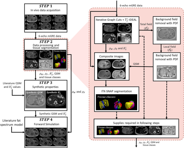
(Left) Pipeline employed in the phantom generation process. (Right) A magnified view shows the detailed workflow of the data processing and tissue segmentation step
2.1. In vivo data acquisition
We scanned a healthy volunteer (24‐y‐old female) in a 3T Philips Ingenia MRI scanner using an 18‐s single breath‐hold multi‐echo 3D GRE sequence. The acquisition parameters were: number of echoes = 6, TE1 = 1.8 ms, TE = 1.56 ms, TR = 10.76 ms, flip angle = 10°, FOV = 380 × 380 × 180 mm3, matrix size = 192 × 192 × 90, voxel size = 1.98 × 1.98 × 2 mm3, bandwidth = 2222 Hz/pixel, and SENSE reduction factor = 2. The acquisition was performed after an informed consent was signed by the volunteer and under the approval of the Institutional Ethics Committee.
2.2. Data processing and tissue segmentation
The main purpose of this step is to obtain the inputs employed in the generation of the synthetic properties and in the forward simulation. The experimental MR properties (, , , and QSM) and the tissue class labels were obtained following a series of interconnected processes (Figure 1, right hand side). Phase unwrapping and chemical shift removal of the acquired GRE MR images were performed using the IGC approach from the ISMRM fat‐water toolbox. 38 The , , , and a refined fieldmap were obtained using ‐IDEAL with a six‐peak fat model. 38 , 39
Additionally, we decided to compute a QSM from experimental data to (i) use it as an auxiliary segmentation reference for hepatic vessels, (ii) to provide susceptibility values for non‐reported tissues, and (iii) for visual comparison with our synthetic phantom. First, we generated a binary mask using the combined , , and echo magnitude images, excluding the arms and the internal air regions from lungs and gastrointestinal tract. Then, we applied the projection onto dipole fields (PDF) algorithm 37 to remove the background contributions from the fieldmap derived from the water‐fat separation process. No further erosion processes were made. We performed the dipole inversion using FAst Nonlinear Susceptibility Inversion (FANSI). 34
Composite images were generated using the magnitude images of the echoes, and , QSM, and maps. These images were employed to perform the tissue segmentations with the ITK‐Snap (version 3.8) active contours function. 40 We automatically segmented 23 structures of the abdominal region and we manually refined them. The segmented structures were the aorta, inferior vena cava, right kidney, left kidney, liver, spleen, gallbladder, esophagus, stomach, pancreas, small intestine, large intestine, hepatic veins, portal vein, ribs, vertebrae, intervertebral disks, spinal cord, subcutaneous fat, visceral fat, heart, muscle, and air regions inside the gastrointestinal tract and lungs.
2.3. Synthetic properties
We used the segmentations and properties obtained in the previous stage to generate two synthetic maps: susceptibility and . In both cases, the map values were assigned within a similar range as that provided by the reference images (experimental QSM and maps) and the literature (healthy or pathologic cases), while increasing textures and structural details.
2.3.1. Synthetic susceptibility map
A series of spherical ROIs, with radii from three to six pixels, were defined to compute the mean experimental susceptibility of each tissue class (Experimental QSM in Table 1). These ROIs were defined over regions with smooth and stable values, away from streaking artifacts or residual background fields. Air regions and large intestine were masked out in this process. The heart was also excluded to avoid cardiac motion artifacts. Muscle tissue was considered as the zero‐reference under the assumption that it does not accumulate iron, 15 , 16 , 41 and the susceptibility of the esophagus was set to 0, assuming that it is only made of muscular tissue.
TABLE 1.
Reference values and model parameters used to generate the synthetic susceptibility phantoms HS and PL
| Reference values | Synthetic susceptibility model | ||||||
|---|---|---|---|---|---|---|---|
| Reported | Experimental | HS | PL | ||||
| Tissue | QSM (ppm) | QSM (ppm) | (ppm) | (ppm) | (ppm) | (ppm) | (ppm) |
| Aorta | −0.085 41 | 0.044 ± 0.056 | 0.050 | 0.088 | 0.151 | −0.412 | 0.292 |
| Inferior vena cava | 0.054 — 0.445 4 , 63 | 0.424 ± 0.035 | 0.424 | 0.295 | 0.271 | 0.231 | 1.176 |
| Right kidney | 0.03 — 0.11 16 | 0.252 ± 0.144 | 0.180 | 0.255 | 0.091 | 1.437 | 0.111 |
| Left kidney | 0.25 — 0.13 16 | 0.189 ± 0.061 | 0.150 | 0.257 | 0.472 | 0.874 | 0.271 |
| Liver | 0.17 — 0.23 15 , 16 , 41 | 0.123 ± 0.121 | 0.150 | 0.182 | 0.111 | 0.573 | 0.854 |
| Spleen | NR | 0.131 ± 0.129 | 0.130 | 0.181 | 0.091 | 0.030 | 0.653 |
| Gallbladder | NR | 0.179 ± 0.052 | 0.180 | 0.204 | 0.030 | 0.030 | 1.156 |
| Esophagus | NR | 0.164 ± 0.062 | 0 | 0.125 | 0.171 | 0.653 | 0.271 |
| Stomach | NR | 0.170 ± 0.117 | 0.170 | 0.126 | 0.050 | 0.050 | 0.452 |
| Pancreas | NR | 0.074 ± 0.179 | 0.070 | 0.096 | 0.352 | 1.015 | 0.010 |
| Small intestine | NR | 0.172 ± 0.126 | 0.180 | 0.159 | 0.111 | 0.513 | 0.312 |
| Large intestine | 4.84 64 | — | 4.84 | 4.84 | 0 | 0 | 0 |
| Hepatic veins | 0.054 — 0.445 4 , 63 | 0.367 ± 0.068 | 0.367 | 0.309 | 0.472 | 0.332 | 0.794 |
| Porta vein | 0.054 — 0.445 4 , 63 | 0.343 ± 0.040 | 0.343 | 0.266 | 0.131 | 0.814 | 1.096 |
| Ribs | 2.4 — 1.4 35 , 65 | 0.901 ± 0.248 | 1.200 | 0.109 | 0.030 | 0.412 | 0.975 |
| Vertebrae | 0.037 — 0.032 66 | 0.372 ± 0.250 | 0.050 | 0.004 | 0.111 | 0.251 | 1.055 |
| Intervertebral disks | NR | 0.176 ± 0.069 | 0.180 | 0.050 | 0.050 | 0.312 | 0.633 |
| Spinal cord | NR | 0.135 ± 0.173 | 0.140 | 0.088 | 0.010 | 0.352 | 0.714 |
| Subcutaneous fat | 0.6 — 0.7 23 , 41 | 0.517 ± 0.155 | 0.550 | 0.215 | 0.372 | 0.111 | 0.171 |
| Visceral fat | 0.6 — 0.7 23 , 41 | 0.741 ± 0.200 | 0.700 | 0.344 | 0.251 | 0.714 | 0.452 |
| Heart | NR | — | 0 | 0 | 0 | 0 | 0 |
| Muscle | 0 | 0 | 0 | 0 | 0.292 | 1.156 | 0.533 |
| Internal Air | 4.84 64 | — | 4.84 | 4.84 | 0 | 0 | 0 |
| External Air | 9.2 35 | — | 9.2 | 9.2 | 0 | 0 | 0 |
Note: (i) NR stands for non‐reported susceptibility values. (ii) The texture of 0‐fixed tissues (muscle and esophagus) was also modulated to avoid constant value regions. (iii) The experimental QSM value of muscle tissue was −0.226 ± 0.030 ppm. The References values column shows the Reported QSM values from the literature and the Experimental QSM values for HS, obtained from small ROIs as described in the Synthetic properties section.
Since the literature showed both, some variability in terms of the reported tissue susceptibilities and sometimes some inconsistencies with our experimental values (Table 1), we considered the following rules. If the experimental mean was consistent with the range reported in the literature, we used the computed value as the mean susceptibility of the tissue. If the experimental values were outside the literature range, the assigned mean susceptibility was a value between the experimental mean and the range limit, keeping it as close as possible to the latter. For the case of non‐reported tissues (e.g., spleen, stomach, and pancreas), we set the value of the mean susceptibility obtained from our experimental QSM, rounded to the second decimal place.
To avoid promoting over‐regularized solutions and to provide realistic textures for the synthetic QSM, we employed a similar strategy as that used in RC2. 35 However, instead of using and , the susceptibility of each voxel was modulated using , and . This heuristic was chosen based in the linear dependence found between and iron concentration, 12 , 13 and between susceptibility and PDFF 42 Additionally, this formulation gives the practical advantage of separately modulate the textures related to water and fat structures in a same tissue class. To reduce scaling problems due to differences in the magnitude range of , , and we normalized each of these parameters in the 0 to 1 range, resulting in , , and , respectively. We then defined the susceptibility with the following equation:
| (1) |
where is the synthetic susceptibility of the tissue class at the voxel , is the assigned mean susceptibility, and , , and are the mean values taken from the whole mask of the tissue class . The initial values of the texture modulation weighting parameters , , and were found by minimizing the normalized RMS error (nRMSE) between the synthetic susceptibility and the experimental QSM for every tissue class. Then, parameter values were manually adjusted, following a visual inspection heuristic, which consisted in increasing texture and structural details (e.g., small vessels and muscle fibers), commonly attenuated in the experimental QSM map due to over‐regularization. We modified the values of , , and to slightly increase the structural contrast, while avoiding the generation of piece‐wise constant tissue classes.
Sharp tissue transitions become unrealistic for an abdominal scenario. Tissue interphases are commonly smooth due to partial volume effects at the low acquisition resolutions employed for the abdomen. To reproduce these effects, we applied the approach described in RC2. 35 A Gaussian kernel with = 0.5 was applied to each tissue class mask, except for hepatic veins, portal vein, large intestine, heart, and air regions. The probability that a voxel belongs to a tissue class was calculated by dividing each resulting mask by the total sum of all tissue masks . Then,
| (2) |
2.3.2. Synthetic map
For several pathologies, compromised tissues present significant changes not only in susceptibility values, but also in terms of signal decay, 43 which results in signal void regions with poor SNR. We therefore defined a model to create a synthetic map based on the same expression of Eq. (1) but setting and to 0. Thus:
| (3) |
where is the synthetic value of the tissue class at the voxel , and is the mean value assigned to the tissue class . The value of the parameter was chosen so that the resulting map acquired a realistic non‐smooth texture. When no changes are needed (), the value is set as the experimental one. Otherwise, for each tissue class the value is modified to an arbitrary value set by the user, to re‐create pathological scenarios.
2.4. Forward simulation
This is the final step of the phantom generation workflow, where the synthetic and maps are integrated into a signal model that also includes fat contributions. To eliminate the regions with fat swaps or lack of signal, we cropped five proximal and five distal axial slices of the complex water and fat images ( and ) leaving a final matrix size of 192 × 192 × 80. The same cropping was applied to and .To simulate a complex acquired signal, we neglected and flip angle effects. Fat contributions were introduced into our signal model as a six‐peak model 38 with frequency shifts () of −3.8, −3.4, −2.6, −1.94, −0.39, 0.6 ppm and relative amplitudes () of 0.087, 0.693, 0.128, 0.004, 0.039, 0.048, respectively. The single‐ multipeak water‐fat signal model which describes the evolution of a voxel with time has been widely studied 19 , 20 , 22 , 44 and can be formulated as follows:
| (4) |
where is the signal value of the voxel at the ‐th TE (), is the field strength, and is the gyromagnetic ratio. The fieldmap can be modeled as the 3D convolution of the local and background synthetic susceptibility maps with a magnetic dipole kernel along the z‐axis direction, which can be computed as a point‐wise multiplication in the Fourier domain. 45 , 46
| (5) |
with and the direct and inverse Fourier transform, respectively.
Instead of using the classical continuous formulation, 45 , 46 we employed a discrete approach 47 and zero‐padding by a factor of 2 along each dimension. This alternative formulation reduces aliasing artifacts that appear around regions with abrupt susceptibility variations (e.g., fat, bone, and air interfaces), which are originated by the sampling processes. 48
2.5. Phantom generation
2.5.1. Synthetic maps scenarios
To verify the ability of our phantom to simulate different susceptibility and values, we defined three scenarios:
Healthy subject (HS): values were assigned following the procedure described in the Synthetic susceptibility map section. In this case, the map was kept as the experimental one for every tissue class.
Pathologic lobe (PL): This scenario aims at showing the behavior of the phantom when all susceptibility values were slightly modified, while values increase significantly. In this case, each value was assigned as the mean value of the experimental QSM, instead of spherical ROIs described in the Synthetic susceptibility map section. These alternative values were taken from the whole mask of the tissue class , similar as , , and in Eq. (1). The values of susceptibility model parameters , , were the same as in HS. We simulated a lobe with a mean value of 150 and a mean susceptibility value of 0.2 ppm located in the liver, close to the porta hepatis. For the rest of the tissues, the values were the same as in HS.
Iron overload (IO): This phantom simulates a pathologic scenario, where and values were drastically increased for the affected tissues. Liver, spleen, pancreas, and vertebrae were chosen as the compromised tissues, as they all can be observed in a single slice. This represents a realistic scenario for hemochromatosis or hemosiderosis, where iron overload occurs in the liver, spleen, pancreas, and bone marrow, causing higher susceptibility values and a faster decay. 43 In this case, the susceptibility model parameters , , and were set manually, attempting to reproduce realistic textures. For non‐affected tissues, the values of those parameters were the same as in HS.
Table 1 shows the reference values and the model parameters employed in the generation of HS and PL. Table 2 shows the susceptibility and model parameters employed in IO.
TABLE 2.
Synthetic susceptibility and model parameters employed for the IO phantom
| Synthetic susceptibility model | Synthetic model | |||||
|---|---|---|---|---|---|---|
| Tissue | (ppm) | (ppm) | (ppm) | (ppm) | (Hz) | (Hz) |
| Liver | 0.60 | 0.332 | 0.719 | 0.854 | 100 | 225 |
| Spleen | 0.28 | 0.226 | 0.076 | 0.653 | 54 | 100 |
| Pancreas | 0.20 | 0.528 | 1.523 | 0.015 | 57 | 110 |
| Vertebrae | 0.05 | 0.111 | 0.251 | 1.055 | 145 | 200 |
To simulate the background field effects, we considered the external air, the large intestine and the gases from the gastrointestinal tract as background susceptibility sources. In order to reproduce a realistic background scenario, we appended axial‐flipped copies of our phantom in the axial direction, to emulate the superior and inferior regions of the body outside the phantom ROI. We also zero‐padded along the sagittal and coronal directions, resulting in a matrix size of 576 × 576 × 240. Then, we performed the dipole convolution and cropped the resulting field to its original size.
2.5.2. Simulated acquisitions
We simulated two acquisition protocols, which correspond to two of the most common approaches employed for abdominal QSM: water/fat separation and in‐phase acquisitions. The former consists in acquiring a series of echoes at a short and regular TE spacing and estimate the fieldmap using iterative algorithms like IGC. The latter approach sets the acquisitions at the TEs when water and fat are in the same phase. These TEs are commonly defined using a single‐peak fat model assumption, which results in echo acquisitions at every 2.3 ms for a 3T scanner. Given the signal model of Eq. (4), the simulation of these protocols is straight‐forward, and it just needs to set the TEs, defined as follows:
Protocol 1 (P1): Six‐echo acquisition with the same TEs as the experimental data: TE1 = 1.8 ms and TE = 1.56 ms. With this protocol we performed a QSM pipeline with a chemical shift correction step and compared the simulated phantom appearance with the experimental data.
Protocol 2 (P2): Five in‐phase echoes with TE1 = 2.3 ms and TE = 2.3 ms. With this protocol we performed a direct QSM reconstruction approach, without need of any chemical‐shift correction.
2.6. Experimental validation
For this implementation, we assumed a perfect background‐field removal. Thus, all voxels corresponding to air regions and large intestine were set to 0 and masked out from the synthetic maps and the signal model (). The synthetic susceptibility phantom was demeaned and forward‐simulated as described in Eq. (4). We decided to keep the phase contributions of fat, to study how the errors from the water/fat separation and in‐phase approaches propagate and affect the QSM reconstructions.
We performed the dipole inversion with five different methods reported in literature: Morphological Enabled Dipole Inversion (MEDI), 49 STreaking Artifact Reduction (STAR‐QSM), 50 , 51 Nonlinear Dipole Inversion (NDI), 52 FANSI, 34 , 53 and Hybrid Data fidelity term approach for QSM (HD‐QSM). 54 To evaluate our phantom as a ground truth for the assessment of QSM algorithms, we compared the quality of the obtained reconstructions under two different schemes:
QSM with chemical shift correction: Using data from P1, we performed a chemical shift correction and a water/fat separation with IGC 22 and T2*‐IDEAL. 39 The resulting fieldmap was employed as input for the dipole inversion. For NDI, FANSI, and HD‐QSM we defined a magnitude‐based and spatially variable weight for the data fidelity as:
| (6) |
where N is the number of echoes.
Direct QSM: Using data from P2, we performed a standard QSM pipeline. This includes phase unwrapping with ROMEO, 55 a linear least squared multi‐echo fit, and then dipole inversion. For the data fidelity term (NDI, FANSI, and HD‐QSM), we considered the spatially variable weight , defined in Eq. (6).
We added normally distributed complex noise () to the simulated data, with a peak SNR of 100. Reconstructed fieldmaps, maps and QSM maps were compared against ground truths using the nRMSE metric. To compare QSM reconstructions, we also employed the QSM‐specific structural similarity metric (XSIM). 56 To obtain the optimal QSM reconstructions (NDI, MEDI, FANSI, and HD‐QSM), parameters were set as those that minimize nRMSE.
3. RESULTS
3.1. Phantom simulations
Figure 2 shows a comparison between experimental data and the three synthetic phantoms. The first row shows an axial slice of the experimental susceptibility and the synthetic susceptibilities for phantoms HS, PL, and IO. HS shows a high contrast between the different tissue classes and texture details in tissues like pancreas, muscle, kidney, and visceral fat. In PL, instead of using specific ROIs, the mean susceptibilities were assigned as the average values inside each tissue class. This resulted in lower contrast between the tissue classes, especially in the bone/muscle, muscle/fat, and organ/fat transitions. The IO phantom aimed to simulate an iron overload scenario, with iron accumulations in the liver, spleen, pancreas, and vertebrae, as can be seen in the top‐right of Figure 2. Here, the liver shows a significant susceptibility increase, whereas smaller increases occur for the rest of the compromised tissues.
FIGURE 2.
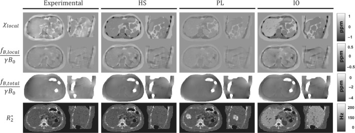
Representative axial and sagittal slices of the susceptibility, local field, total field, and maps of the experimental data and the three simulated phantoms: HS, PL, and IO
The second and third rows of Figure 2 show axial and sagittal slices of the resulting local and total fieldmaps after performing the convolution with the dipole kernel. For local fieldmaps, HS and IO present a similar level of detail as that in the experimental case, with higher contrast in the muscle/bone interphase and in the hepatic veins of IO. In the case of PL, the assigned values of muscle, ribs, and fat are closer to each other (Table 1), which results in a smoother transition between these tissue classes with no hyperintense regions around the ribs, in contrast to experimental data, HS, and IO. For total fieldmaps, the three phantoms show a similar appearance compared to the experimental case, except for the two hyperintense regions around the masked intestines and at the posterior‐left side of the phantoms.
The last row of Figure 2 shows the synthetic maps. For HS, map is the same as in the experimental case. For PL and IO, the maps show increased values for the simulated lobe and the iron overload in the chosen tissues, while keeping similar textures compared with the experimental case.
Figure 3 shows the resulting magnitudes and the unwrapped phases using ROMEO 55 for the three phantoms, after performing the forward simulation with the acquisition protocols P1 and P2. On the one hand, for all phantoms the phase of P1 acquisitions shows a similar appearance as that of the experimental case at the first echoes, with the same exceptions mentioned for Figure 2. For higher TEs, phase images become different compared to the experimental case, with hyperintense regions surrounding the subcutaneous fat. These differences might be explained by the simplifications made for modeling the background susceptibility sources. On the other hand, P1 magnitude images are almost identical to those of the experimental case, particularly the same out‐of‐phase artifacts at the muscle/fat interphases and at the right‐hand side of the pancreas at . For PL and IO images, a faster signal decay is observed in the simulated lobe and the tissues with iron overload: liver, spleen, pancreas, and vertebrae.
FIGURE 3.
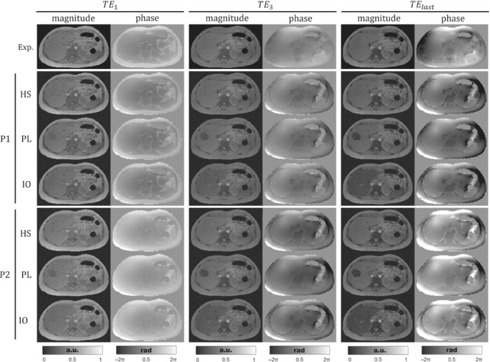
Axial views of the experimental and simulated acquired signals for phantoms HS, PL, and IO with protocols P1 and P2. The three pairs of columns show magnitude and the unwrapped phase at the first, third, and last TE (sixth echo for P1 or fifth for P2), respectively. To ease visualization, magnitude images were normalized between 0 and 1.
Protocol P2 was defined to simulate in‐phase acquisitions. In the first TE, the above‐mentioned out‐of‐phase artifacts are significantly reduced for P2 magnitude images. Additionally, the P2 phase image at shows a reduced water/fat contrast compared with P1 and the experimental data. For experimental data and P1, the third and last TEs are close to in‐phase acquisition times ( = 4.92 ms and = 9.6 ms). As consequence, experimental data, HS‐P1, and HS‐P2 show similar magnitude and phase images for and . The last echo phase image of P2 starts showing a higher contrast between fat and water structures; this can be clearly seen in the fat/muscle interphase.
3.2. Phantom reconstructions
Figure 4(A) shows the estimated total fieldmaps (HS, PL, and IO) for the two strategies associated to P1 and P2. For the in‐phase protocol, total fieldmap estimations using ROMEO and multiecho fitting results in smooth and continuous fieldmaps without phase wrap errors. However, IGC estimations for P1 show several fieldmap errors in some regions (pointed by black arrows), showing the sensitivity of the algorithm under the presence of strong fieldmap inhomogeneities. Given the significative differences between P1 and P2 total field estimations, we decided to ignore this step for the subsequent QSM reconstructions, and assume a perfect background field removal scenario, as described in the Experimental validation section.
FIGURE 4.
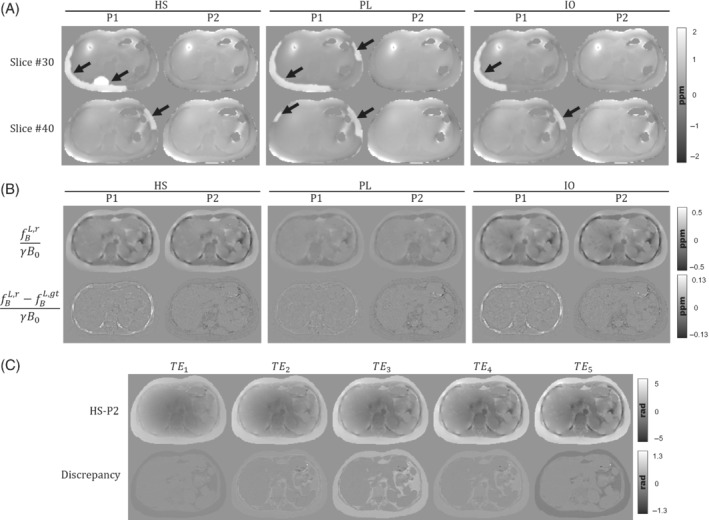
(A) Two axial examples of the total fieldmap estimations of phantoms HS, PL, and IO, for the corresponding acquisition protocols P1 and P2. Estimation errors from IGC can be seen as hyperintense regions around the subcutaneous fat (black arrows). (B) Axial slices of the local field reconstructions for phantoms HS, PL, and IO, and their difference with ground truth. Left and right columns show the results for P1 and P2 protocols, respectively. (C) Unwrapped phase of the HS phantom with the one‐peak‐based in‐phase protocol (P2) and its discrepancies with a perfect in‐phase simulation at every TE
Figure 4(B) shows the reconstructed local fieldmaps for both protocols and their respective differences against ground truths. For the three phantoms, reconstructions with protocol P1 produce fieldmaps with overestimated values in the ribs. This might be caused by residual errors from IGC and ‐IDEAL that might propagate to the dipole inversion step. Reconstructions with protocol P2 show structural differences in the fatty tissue regions (i.e., subcutaneous fat, visceral fat, and bone marrow in vertebrae). We compared the one‐peak based acquisitions of HS‐P2 against a perfect in‐phase simulation where we forced for each in Eq. (4). The difference maps of Figure 4(C) show the discrepancies generated under the one‐peak based in‐phase assumption, where the main differences can be appreciated in the fat‐related tissues.
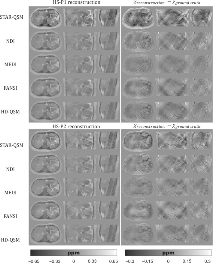
Figures 5, 6, 7 show the QSM reconstructions of the HS, PL, and IO phantoms. For HS, PL, and IO, the STAR‐QSM and NDI reconstructions present several streaking artifacts around ribs and vertebrae. With MEDI, FANSI, and HD‐QSM, reconstructions show a significant reduction of streaking artifacts, but also some dark regions around the ribs and a loss of structural information in the regions surrounding the stomach, intestine, left kidney, ribs, and vertebrae. Whereas STAR‐QSM present larger susceptibility values for the ribs and subcutaneous fat compared to the ground truth, the other reconstruction algorithms present smaller susceptibility values, resulting in hyperintense structures in the difference images, especially with NDI. For the above‐mentioned regions, P1 reconstructions present larger structural errors than P2. This might be a consequence of error propagation from the previous fieldmap estimation step with IGC and ‐IDEAL. Nevertheless, it is interesting how STAR‐QSM manages to address that problem in P1 but generates the opposite problem in P2, with hypointense regions around the whole rib cage.
FIGURE 5.

(Left) Axial, coronal, and sagittal slices of QSM reconstructions for the HS phantom with P1 (top) and P2 (bottom). (Right) Axial, coronal, and sagittal slices with the difference between the reconstructed QSM image and the ground truth
FIGURE 6.
(Left) Axial, coronal, and sagittal slices of QSM reconstructions for the PL phantom with P1 (top) and P2 (bottom). (Right) Axial, coronal, and sagittal slices with the difference between the reconstructed QSM image and the ground truth
FIGURE 7.

(Left) Axial, coronal, and sagittal slices of QSM reconstructions for the IO phantom with P1 (top) and P2 (bottom). (Right) Axial, coronal, and sagittal slices with the difference between the reconstructed QSM image and the ground truth
Table 3 shows the nRMSE of the reconstructed fieldmaps and maps. It also shows the nRMSE and XSIM of the QSM reconstructions for each evaluated method. For maps and fieldmaps, reconstructions present a similar nRMSE, with slightly higher values for the P2 protocol. In the case of the fieldmap, PL‐P2 presents a significantly higher nRMSE. This might be explained by the presence of unreliable voxels from the phase unwrapping of echo fitting steps, which increase severely the nRMSE but do not affect significantly the respective QSM reconstructions, compared with PL‐P1. Despite having a similar appearance compared with HS and IO reconstructions, PL shows a significant nRMSE increase. This might be explained because of the shorter range of susceptibility values in PL, which decreases the contrast between tissues and increases the effects of noise.
TABLE 3.
Accuracy metrics for the reconstructed fieldmaps, and QSM
| HS | PL | IO | ||||||
|---|---|---|---|---|---|---|---|---|
| P1 | P2 | P1 | P2 | P1 | P2 | |||
| Fieldmap | nRMSE (%) | 14.50 | 19.38 | 18.33 | 40.64 | 14.50 | 18.57 | |
|
|
nRMSE (%) | 13.48 | 14.47 | 13.16 | 14.21 | 12.12 | 12.98 | |
| STAR‐QSM | nRMSE (%) | 51.18 | 52.64 | 82.28 | 71.93 | 54.41 | 55.87 | |
| XSIM | 0.472 | 0.468 | 0.340 | 0.423 | 0.437 | 0.444 | ||
| NDI | nRMSE (%) | 41.80 | 39.84 | 47.38 | 48.85 | 46.10 | 43.50 | |
| XSIM | 0.519 | 0.522 | 0.461 | 0.470 | 0.468 | 0.476 | ||
| MEDI | nRMSE (%) | 25.41 | 22.84 | 36.29 | 35.84 | 30.29 | 27.58 | |
| XSIM | 0.721 | 0.734 | 0.574 | 0.621 | 0.662 | 0.678 | ||
| FANSI | nRMSE (%) | 29.92 | 25.88 | 43.32 | 41.59 | 33.35 | 29.43 | |
| XSIM | 0.659 | 0.704 | 0.525 | 0.561 | 0.611 | 0.655 | ||
| HD‐QSM | nRMSE (%) | 32.56 | 28.94 | 50.42 | 43.29 | 36.64 | 33.08 | |
| XSIM | 0.654 | 0.702 | 0.457 | 0.542 | 0.597 | 0.644 | ||
As qualitatively observed in Figure 5 and Figure 7, the TV regularization‐based methods (MEDI, FANSI, and HD‐QSM) show improved reconstructions compared with STAR‐QSM and NDI, with similar nRMSE and XSIM values around 25%–36% and 0.60–0.75, respectively.
4. DISCUSSION
In this work, we presented a realistic numerical phantom of the abdomen for the evaluation and comparison of different QSM reconstruction methods and pipelines under controlled conditions. The phantom effectively simulates susceptibility and values, and their corresponding magnitude and phase signals considering fat contributions and background susceptibility sources. It shows a realistic texture appearance and out‐of‐phase effects. The publicly available data and source codes were developed in a modular and flexible pipeline, where the different features can be easily included or removed (e.g., background susceptibility sources). This allows users to simulate phantoms with different tissue properties, signal effects, and acquisition TEs.
Our simulation pipeline employs MRI‐based segmentations and a multiparametric model to provide realistic geometries and textures to each of the tissue classes. These features represent an advantage compared with simplified models based in simple geometric shapes, or the current abdominal models with realistic anatomies but piecewise tissue property values. 19 , 36 , 57 Additionally, the fact that synthetic maps can be easily adjusted allows the users to simulate realistic scenarios, where not only the susceptibility but also the signal decay is involved. Both and QSM values can be easily and arbitrary modified, beyond the default parameters described here. Thus, users can modify or correct these rules and values according to their needs.
The addition of fat signal effects represents a new approach for the evaluation of the current outside‐the‐brain QSM pipelines. On the one hand, this feature allows researchers to develop new algorithms for simultaneous QSM in the presence of fat, and to compare different reconstruction pipelines which in some cases require different acquisition times to remove the chemical shift effects (e.g., ‐IDEAL, in‐phase acquisitions, multispectral ARMA modeling, 58 etc.). Our model allows us to define arbitrarily the TEs of the simulated acquisitions. In practice, this can be done simply by specifying the TEs in the header of our source code. On the other hand, this feature, in combination with the simulation of different χ and values, could be used to generate training data for neural‐network‐based aproaches, as proposed by Zhao et al. 36 Additionally, the phantom also includes a fieldmap and a PDFF ground truths, to evaluate, identify, and solve critical stages of the employed pipelines and water‐fat separation methods.
We used a forward simulation scheme to evaluate two of the current outside‐the‐brain QSM pipelines: water‐fat separation and in‐phase acquisition. For water‐fat separation with IGC and ‐IDEAL, phantom reconstructions showed that the algorithm is significatively sensitive to strong fieldmap inhomogeneities, and it is also prone to leave residual errors in regions with drastic susceptibility changes, like ribs and muscle/fat interphases. These errors were propagated to the dipole inversion step and generated systematic structural differences between the reconstructions and the ground truth for most QSM dipole inversion algorithms.
For in‐phase acquisitions, the reconstructed fieldmaps presented structural errors around the fat regions. These errors might be explained by TE mismatch between the one‐peak‐based in‐phase acquisition and the multiple frequency shifts of the six‐peak fat model, causing fat discrepancies as shown in Figure 4(C). Despite being the main clinical workhorse for water and fat images, questions have been raised about the usage of one‐peak‐based acquisitions and how this scheme introduces significant quantifications bias for QSM. 19 In this sense, the effective TEs proposed by Boehm et al. 19 could be employed in a future work, in order to evaluate a potential reduction on these mismatch effects.
QSM reconstruction experiments showed that algorithms like MEDI, FANSI, and HD‐QSM were more robust to noisy voxels and streaking artifacts. However, current algorithms are still prone to errors in regions with drastic susceptibility changes. This could be seen in Figures 5, 6, 7, where structural errors in the ribs were present in both acquisition protocols P1 and P2, despite of being significantly reduced for P2. These results show the potential of our phantom as a ground truth, allowing researchers to identify and solve critical stages of the current QSM pipelines.
There are some limitations in our framework. Due to the absence of an abdominal MRI atlas for the registration of the different tissue classes, the segmentations were performed just for common abdominal structures of a single female individual. Considering anatomical variations would require repeating the entire segmentation process.
Our signal model of Eq. (4) is based in the standard formulation employed in current water/fat separation state‐of‐the‐art studies, 19 , 20 , 22 , 44 which neglect and flip angle effects. Including these effects would be desirable to improve simulations and to allow and compare new acquisition scenarios. However, the incorporation of the previous effects is not straightforward (particularly ) since one would need to generate the corresponding map using the same acquisition as that used for and QSM, and thus, ensuring spatial correspondence among all three parameters may be difficult to achieve. This might be realized by using fingerprinting acquisitions, 59 , 60 which enables fast multiparametric maps (compatible with a breath hold scan) or using self‐navigating sequences 61 that could allow free‐breathing multiparametric acquisitions.
Our simulation corresponds to a static breath‐hold case, without moving artifacts from small respiratory motion. Additionally, the water and fat fractions are also static, leading to just one PDFF case. If necessary, incorporating the respiratory motion might be addressed using a similar model as that proposed by Lo et al. 57 Considering dynamic PDFF might be solved by employing a synthetic PDFF and including it in the signal model formulation of Eq. (4) and its contributions to the synthetic map. 62 The modular framework of our phantom source code allows including these features, and this might be considered as a future work.
5. CONCLUSIONS
We developed a numerical abdominal phantom for QSM, which effectively simulates susceptibility and maps with realistic texture appearance. Our simulation pipeline included two adjustable tissue properties and a signal model that incorporates background fields and fat phase contributions, allowing to recreate different susceptibility and signal scenarios and to mimic some abnormal conditions. Our reconstruction experiments show the potential of our phantom as a ground truth to develop and compare not only QSM algorithms but also water‐fat separation methods.
ACKNOWLEDGMENTS
This research work was funded by Fondecyt 1181057, Fondecyt 1191710, Fondecyt 1231535, Anid/PIA/Anillo ACT192064, and Millennium Institute for Intelligent Healthcare Engineering CN2021_004. Dr Carlos Milovic was supported by Cancer Research UK Multidisciplinary Award C53545/A24348. Dr Cristobal Arrieta was partially funded by ANID Fondecyt Postdoctorado 2019 No. 3190763.
Silva J, Milovic C, Lambert M, et al. Toward a realistic in silico abdominal phantom for QSM. Magn Reson Med. 2023;89:2402‐2418. doi: 10.1002/mrm.29597
Click here for author‐reader discussions
Funding information Agencia Nacional de Investigación y Desarrollo, Grant/Award Numbers: Millennium Science Initiative Program ICN2021_004; PIA‐ACT 192064; Cancer Research UK, Grant/Award Numbers: Multidisciplinary Award C53545/A24348; A24348; C53545; Fondo Nacional de Desarrollo Científico y Tecnológico, Grant/Award Numbers: 1181057; 1191710; 1231535; 3190763
DATA AVAILABILITY STATEMENT
The source code is publicly available at: https://gitlab.com/qsm1/realistic_abdominal_phantom.
REFERENCES
- 1. De Rochefort L, Liu T, Kressler B, et al. Quantitative susceptibility map reconstruction from MR phase data using bayesian regularization: validation and application to brain imaging. Magn Reson Med. 2010;63:194‐206. [DOI] [PubMed] [Google Scholar]
- 2. Haacke EM, Liu S, Buch S, Zheng W, Wu D, Ye Y. Quantitative susceptibility mapping: current status and future directions. Magn Reson Imaging. 2015;33:1‐25. [DOI] [PubMed] [Google Scholar]
- 3. Liu C, Li W, Tong KA, Yeom KW, Kuzminski S. Susceptibility‐weighted imaging and quantitative susceptibility mapping in the brain. J Magn Reson Imaging. 2015;42:23‐41. [DOI] [PMC free article] [PubMed] [Google Scholar]
- 4. Wang Y, Liu T. Quantitative susceptibility mapping (QSM): decoding MRI data for a tissue magnetic biomarker. Magn Reson Med. 2015;73:82‐101. [DOI] [PMC free article] [PubMed] [Google Scholar]
- 5. Langkammer C, Schweser F, Krebs N, et al. Quantitative susceptibility mapping (QSM) as a means to measure brain iron? A post mortem validation study. Neuroimage. 2012;62:1593‐1599. [DOI] [PMC free article] [PubMed] [Google Scholar]
- 6. Chen W, Zhu W, Ii K, et al. Intracranial calcifications and hemorrhages: characterization with quantitative susceptibility mapping. Radiology. 2014;270:496‐505. [DOI] [PMC free article] [PubMed] [Google Scholar]
- 7. Haacke EM, Tang J, Neelavalli J, Cheng YCN. Susceptibility mapping as a means to visualize veins and quantify oxygen saturation. J Magn Reson Imaging. 2010;32:663‐676. [DOI] [PMC free article] [PubMed] [Google Scholar]
- 8. Fan AP, Bilgic B, Gagnon L, et al. Quantitative oxygenation venography from MRI phase. Magn Reson Med. 2014;72:149‐159. [DOI] [PMC free article] [PubMed] [Google Scholar]
- 9. Langkammer C, Liu T, Khalil M, et al. Quantitative susceptibility mapping in multiple sclerosis. Radiology. 2013;267:551‐559. [DOI] [PMC free article] [PubMed] [Google Scholar]
- 10. Chen W, Gauthier SA, Gupta A, et al. Quantitative susceptibility mapping of multiple sclerosis lesions at various ages. Radiology. 2014;271:183‐192. [DOI] [PMC free article] [PubMed] [Google Scholar]
- 11. Langkammer C, Pirpamer L, Seiler S, et al. Quantitative susceptibility mapping in Parkinson's disease. PloS One. 2016;11:e0162460. [DOI] [PMC free article] [PubMed] [Google Scholar]
- 12. Sharma SD, Hernando D, Horng DE, Reeder SB. Quantitative susceptibility mapping in the abdomen as an imaging biomarker of hepatic iron overload. Magn Reson Med. 2015;74:673‐683. [DOI] [PMC free article] [PubMed] [Google Scholar]
- 13. Sharma SD, Fischer R, Schoennagel BP, et al. MRI‐based quantitative susceptibility mapping (QSM) and R2* mapping of liver iron overload: comparison with SQUID‐based biomagnetic liver susceptometry. Magn Reson Med. 2017;78:264‐270. [DOI] [PMC free article] [PubMed] [Google Scholar]
- 14. Jafari R, Hectors SJ, Koehne de González AK, et al. Integrated quantitative susceptibility and R2* mapping for evaluation of liver fibrosis: an ex vivo feasibility study. NMR Biomed. 2021;34:e4412. [DOI] [PMC free article] [PubMed] [Google Scholar]
- 15. Qu Z, Yang S, Xing F, et al. Magnetic resonance quantitative susceptibility mapping in the evaluation of hepatic fibrosis in chronic liver disease: a feasibility study. Quant Imaging Med Surg. 2021;11:1170‐1183. [DOI] [PMC free article] [PubMed] [Google Scholar]
- 16. Bechler E, Stabinska J, Thiel T, et al. Feasibility of quantitative susceptibility mapping (QSM) of the human kidney. Magn Reson Mater Physics, Biol Med. 2021;34:389‐397. [DOI] [PMC free article] [PubMed] [Google Scholar]
- 17. Karsa A, Punwani S, Shmueli K. An optimized and highly repeatable MRI acquisition and processing pipeline for quantitative susceptibility mapping in the head‐and‐neck region. Magn Reson Med. 2020;84:3206‐3222. [DOI] [PubMed] [Google Scholar]
- 18. Liu S, Wang C, Zhang X, et al. Quantification of liver iron concentration using the apparent susceptibility of hepatic vessels. Quant Imaging Med Surg. 2018;8:123‐134. [DOI] [PMC free article] [PubMed] [Google Scholar]
- 19. Boehm C, Schlaeger S, Meineke J, Weiss K, Makowski MR, Karampinos DC. On the water–fat in‐phase assumption for quantitative susceptibility mapping. Magn Reson Med. 2023;89:1068‐1082. [DOI] [PubMed] [Google Scholar]
- 20. Boehm C, Sollmann N, Meineke J, et al. Preconditioned water‐fat total field inversion: application to spine quantitative susceptibility mapping. Magn Reson Med. 2022;87:417‐430. [DOI] [PubMed] [Google Scholar]
- 21. Straub S, Emmerich J, Schlemmer HP, et al. Mask‐adapted background field removal for artifact reduction in quantitative susceptibility mapping of the prostate. Tomography. 2017;3:96‐100. [DOI] [PMC free article] [PubMed] [Google Scholar]
- 22. Hernando D, Kellman P, Haldar JP, Liang ZP. Robust water/fat separation in the presence of large field inhomogeneities using a graph cut algorithm. Magn Reson Med. 2009;63:79‐90. [DOI] [PMC free article] [PubMed] [Google Scholar]
- 23. Dong J, Liu T, Chen F, et al. Simultaneous phase unwrapping and removal of chemical shift (SPURS) using graph cuts: application in quantitative susceptibility mapping. IEEE Trans Med Imaging. 2015;34:531‐540. [DOI] [PubMed] [Google Scholar]
- 24. Bachrata B, Strasser B, Bogner W, et al. Simultaneous multiple resonance frequency imaging (SMURF): fat‐water imaging using multi‐band principles. Magn Reson Med. 2021;85:1379‐1396. [DOI] [PMC free article] [PubMed] [Google Scholar]
- 25. Lin H, Wei H, He N, et al. Quantitative susceptibility mapping in combination with water‐fat separation for simultaneous liver iron and fat fraction quantification. Eur Radiol. 2018;28:3494‐3504. [DOI] [PMC free article] [PubMed] [Google Scholar]
- 26. Liu T, Spincemaille P, de Rochefort L, Kressler B, Wang Y. Calculation of susceptibility through multiple orientation sampling (COSMOS): a method for conditioning the inverse problem from measured magnetic field map to susceptibility source image in MRI. Magn Reson Med. 2009;61:196‐204. [DOI] [PubMed] [Google Scholar]
- 27. Li W, Liu C, Duong TQ, van Zijl PCM, Li X. Susceptibility tensor imaging (STI) of the brain. NMR Biomed. 2017;30:e3540. [DOI] [PMC free article] [PubMed] [Google Scholar]
- 28. Milovic C, Tejos C, Acosta‐Cabronero J, et al. The 2016 QSM challenge: lessons learned and considerations for a future challenge design. Magn Reson Med. 2020;84:1624‐1637. [DOI] [PMC free article] [PubMed] [Google Scholar]
- 29. Hernando D, Cook RJ, Diamond C, Reeder SB. Magnetic susceptibility as a B 0 field strength independent MRI biomarker of liver iron overload. Magn Reson Med. 2013;70:648‐656. [DOI] [PMC free article] [PubMed] [Google Scholar]
- 30. Li J, Lin H, Liu T, et al. Quantitative susceptibility mapping (QSM) minimizes interference from cellular pathology in R2* estimation of liver iron concentration. J Magn Reson Imaging. 2018;48:1069‐1079. [DOI] [PMC free article] [PubMed] [Google Scholar]
- 31. Langkammer C, Bredies K, Poser BA, et al. Fast quantitative susceptibility mapping using 3D EPI and total generalized variation. Neuroimage. 2015;111:622‐630. [DOI] [PubMed] [Google Scholar]
- 32. Wisnieff C, Liu T, Spincemaille P, Wang S, Zhou D, Wang Y. Magnetic susceptibility anisotropy: cylindrical symmetry from macroscopically ordered anisotropic molecules and accuracy of MRI measurements using few orientations. Neuroimage. 2013;70:363‐376. [DOI] [PMC free article] [PubMed] [Google Scholar]
- 33. Langkammer C, Schweser F, Shmueli K, et al. Quantitative susceptibility mapping: report from the 2016 reconstruction challenge. Magn Reson Med. 2018;79:1661‐1673. [DOI] [PMC free article] [PubMed] [Google Scholar]
- 34. Milovic C, Bilgic B, Zhao B, Acosta‐Cabronero J, Tejos C. Fast nonlinear susceptibility inversion with variational regularization. Magn Reson Med. 2018;80:814‐821. [DOI] [PubMed] [Google Scholar]
- 35. Marques JP, Meineke J, Milovic C, et al. QSM reconstruction challenge 2.0: a realistic in silico head phantom for MRI data simulation and evaluation of susceptibility mapping procedures. Magn Reson Med. 2021;86:526‐542. [DOI] [PMC free article] [PubMed] [Google Scholar]
- 36. Zhao R, Buelo CJ, Velikina JV, et al. Quantitative susceptibility mapping of liver iron overload using deep learning. In: Proceedings of the 30 th Annual Meeting of ISMRM [Virtual]; International Society for Magnetic Resonance in Medicine (ISMRM); 2021:3996. [Google Scholar]
- 37. Liu T, Khalidov I, de Rochefort L, et al. A novel background field removal method for MRI using projection onto dipole fields (PDF). NMR Biomed. 2011;24:1129‐1136. [DOI] [PMC free article] [PubMed] [Google Scholar]
- 38. Hu HH, Börnert P, Hernando D, et al. ISMRM workshop on fat‐water separation: insights, applications and progress in MRI. Magn Reson Med. 2012;68:378‐388. [DOI] [PMC free article] [PubMed] [Google Scholar]
- 39. Yu H, McKenzie CA, Shimakawa A, et al. Multiecho reconstruction for simultaneous water‐fat decomposition and T2* estimation. J Magn Reson Imaging. 2007;26:1153‐1161. [DOI] [PubMed] [Google Scholar]
- 40. Yushkevich PA, Piven J, Hazlett HC, et al. User‐guided 3D active contour segmentation of anatomical structures: significantly improved efficiency and reliability. Neuroimage. 2006;31:1116‐1128. [DOI] [PubMed] [Google Scholar]
- 41. Jafari R, Sheth S, Spincemaille P, et al. Rapid automated liver quantitative susceptibility mapping. J Magn Reson Imaging. 2019;50:725‐732. [DOI] [PMC free article] [PubMed] [Google Scholar]
- 42. Bray TJP, Karsa A, Bainbridge A, et al. Association of bone mineral density and fat fraction with magnetic susceptibility in inflamed trabecular bone. Magn Reson Med. 2019;81:3094‐3107. [DOI] [PMC free article] [PubMed] [Google Scholar]
- 43. Labranche R, Gilbert G, Cerny M, et al. Liver iron quantification with MR imaging: a primer for radiologists. Radiographics. 2018;38:392‐412. [DOI] [PubMed] [Google Scholar]
- 44. Yu H, Shimakawa A, McKenzie CA, Brodsky E, Brittain JH, Reeder SB. Multiecho water‐fat separation and simultaneous R2* estimation with multifrequency fat spectrum modeling. Magn Reson Med. 2008;60:1122‐1134. [DOI] [PMC free article] [PubMed] [Google Scholar]
- 45. Salomir R, de Senneville BD, Moonen CTW. A fast calculation method for magnetic field inhomogeneity due to an arbitrary distribution of bulk susceptibility. Concepts Magn Reson. 2003;19B:26‐34. [Google Scholar]
- 46. Marques JP, Bowtell R. Application of a Fourier‐based method for rapid calculation of field inhomogeneity due to spatial variation of magnetic susceptibility. Concepts Magn Reson Part B Magn Reson Eng. 2005;25B:65‐78. [Google Scholar]
- 47. Milovic C, Acosta‐Cabronero J, Pinto JM, et al. A new discrete dipole kernel for quantitative susceptibility mapping. Magn Reson Imaging. 2018;51:7‐13. [DOI] [PubMed] [Google Scholar]
- 48. Cheng YCN, Neelavalli J, Haacke EM. Limitations of calculating field distributions and magnetic susceptibilities in MRI using a Fourier based method. Phys Med Biol. 2009;54:1169‐1189. [DOI] [PMC free article] [PubMed] [Google Scholar]
- 49. Liu T, Liu J, de Rochefort L, et al. Morphology enabled dipole inversion (MEDI) from a single‐angle acquisition: comparison with COSMOS in human brain imaging. Magn Reson Med. 2011;66:777‐783. [DOI] [PubMed] [Google Scholar]
- 50. Wei H, Dibb R, Zhou Y, et al. Streaking artifact reduction for quantitative susceptibility mapping of sources with large dynamic range. NMR Biomed. 2015;28:1294‐1303. [DOI] [PMC free article] [PubMed] [Google Scholar]
- 51. Chan KS, Marques JP. SEPIA—susceptibility mapping pipeline tool for phase images. Neuroimage. 2021;227:117611. [DOI] [PubMed] [Google Scholar]
- 52. Polak D, Chatnuntawech I, Yoon J, et al. Nonlinear dipole inversion (NDI) enables robust quantitative susceptibility mapping (QSM). NMR Biomed. 2020;33:e4271. [DOI] [PMC free article] [PubMed] [Google Scholar]
- 53. Bilgic B, Chatnuntawech I, Langkammer C, Setsompop K. Sparse methods for quantitative susceptibility mapping. In: Papadakis M, Goyal VK, van De Ville D, eds. Wavelets and Sparsity XVI, SPIE. Vol 9597. SPIE; 2015:959711. [Google Scholar]
- 54. Lambert M, Tejos C, Langkammer C, Milovic C. Hybrid data fidelity term approach for quantitative susceptibility mapping. Magn Reson Med. 2022;88:962‐972. [DOI] [PMC free article] [PubMed] [Google Scholar]
- 55. Dymerska B, Eckstein K, Bachrata B, et al. Phase unwrapping with a rapid opensource minimum spanning tree algorithm (ROMEO). Magn Reson Med. 2021;85:2294‐2308. [DOI] [PMC free article] [PubMed] [Google Scholar]
- 56. Milovic C, Tejos C, Irarrazaval P. Structural similarity index metric setup for QSM applications (XSIM). In: Proceedings of the 5 th International Workshop on MRI Phase Contrast & Quantitative Susceptibility Mapping, Seoul, Korea; 2019. [Google Scholar]
- 57. Lo W, Chen Y, Jiang Y, et al. Realistic 4D MRI abdominal phantom for the evaluation and comparison of acquisition and reconstruction techniques. Magn Reson Med. 2019;81:1863‐1875. [DOI] [PMC free article] [PubMed] [Google Scholar]
- 58. Tipirneni‐Sajja A, Loeffler RB, Hankins JS, Morin C, Hillenbrand CM. Quantitative susceptibility mapping using a multispectral autoregressive moving average model to assess hepatic iron overload. J Magn Reson Imaging. 2021;54:721‐727. [DOI] [PMC free article] [PubMed] [Google Scholar]
- 59. Jaubert O, Cruz G, Bustin A, et al. T1, T2, and fat fraction cardiac MR fingerprinting: preliminary clinical evaluation. J Magn Reson Imaging. 2021;53:1253‐1265. [DOI] [PubMed] [Google Scholar]
- 60. Boyacioglu R, Wang C, Ma D, McGivney DF, Yu X, Griswold MA. 3D magnetic resonance fingerprinting with quadratic RF phase. Magn Reson Med. 2021;85:2084‐2094. [DOI] [PubMed] [Google Scholar]
- 61. Küstner T, Bustin A, Jaubert O, et al. Fully self‐gated free‐running 3D cartesian cardiac CINE with isotropic whole‐heart coverage in less than 2 min. NMR Biomed. 2021;34:e4409. [DOI] [PubMed] [Google Scholar]
- 62. Mamidipalli A, Hamilton G, Manning P, et al. Cross‐sectional correlation between hepatic R2* and proton density fat fraction (PDFF) in children with hepatic steatosis. J Magn Reson Imaging. 2018;47:418‐424. [DOI] [PMC free article] [PubMed] [Google Scholar]
- 63. Wen Y, Nguyen TD, Liu Z, et al. Cardiac quantitative susceptibility mapping (QSM) for heart chamber oxygenation. Magn Reson Med. 2018;79:1545‐1552. [DOI] [PMC free article] [PubMed] [Google Scholar]
- 64. Gimsa J, Haberland L. Electric and magnetic fields in cells and tissues. Encycl Condens Matter Phys. 2005;2:6‐14. [Google Scholar]
- 65. Dimov AV, Liu Z, Spincemaille P, Prince MR, Du J, Wang Y. Bone quantitative susceptibility mapping using a chemical species‐specific R2* signal model with ultrashort and conventional echo data. Magn Reson Med. 2018;79:121‐128. [DOI] [PubMed] [Google Scholar]
- 66. Guo Y, Liu Z, Wen Y, et al. Quantitative susceptibility mapping of the spine using in‐phase echoes to initialize inhomogeneous field and R2* for the nonconvex optimization problem of fat‐water separation. NMR Biomed. 2019;32:e4156. [DOI] [PubMed] [Google Scholar]
Associated Data
This section collects any data citations, data availability statements, or supplementary materials included in this article.
Data Availability Statement
The source code is publicly available at: https://gitlab.com/qsm1/realistic_abdominal_phantom.