

Abstract
Background and objective
T-wave alternans (TWA) is a fluctuation of the ST–T complex of the surface electrocardiogram (ECG) on an every–other–beat basis. It has been shown to be clinically helpful for sudden cardiac death stratification, though the lack of a gold standard to benchmark detection methods limits its application and impairs the development of alternative techniques. In this work, a novel approach based on machine learning for TWA detection is proposed. Additionally, a complete experimental setup is presented for TWA detection methods benchmarking.
Methods
The proposed experimental setup is based on the use of open-source databases to enable experiment replication and the use of real ECG signals with added TWA episodes. Also, intra-patient overfitting and class imbalance have been carefully avoided. The Spectral Method (SM), the Modified Moving Average Method (MMA), and the Time Domain Method (TM) are used to obtain input features to the Machine Learning (ML) algorithms, namely, K Nearest Neighbor, Decision Trees, Random Forest, Support Vector Machine and Multi-Layer Perceptron.
Results
There were not found large differences in the performance of the different ML algorithms. Decision Trees showed the best overall performance (accuracy , precision , Recall , F1 score ). Compared to the SM (accuracy 0.79, precision 0.93, Recall 0.64, F1 score 0.76) there was an improvement in every metric except for the precision.
Conclusions
In this work, a realistic database to test the presence of TWA using ML algorithms was assembled. The ML algorithms overall outperformed the SM used as a gold standard. Learning from data to identify alternans elicits a substantial detection growth at the expense of a small increment of the false alarm.
Keywords: Machine Learning (ML), Spectral Method (SM), Modified Moving Average Method (MMA), Time Method (TM), Cross Validation (CV), Repolarization, T–Wave Alternans (TWA), Electrocardiogram (ECG)
1. Introduction
T–wave alternans (TWA) is a beat-to-beat fluctuation in the repolarization morphology of the electrocardiogram (ECG). It can be manifested as a variation in the amplitude, duration, or waveform of the ST–T complex. Several studies relate cardiac risk and increased malignant arrhythmias to the presence of TWA [1], [2], hence, TWA has been suggested as a marker of sudden cardiac death risk [3], [4], [5].
A variety of methods have been proposed for TWA detection and estimation relying on different techniques. In the Spectral Method [1] ECG beats are segmented and aligned. Then, the periodogram is obtained for each beat-to-beat series and the averaged power spectrum is computed at 0.5 cycles-per-beat (cpb). The resulting value is compared with the spectral noise level to decide if TWA is present. The SM has been extensively used for clinical research and it is included in commercial equipment. In the Complex Demodulation method [6] the ECG beats are aligned, and TWA is represented in each beat series as a sinusoidal signal of cpb with variable amplitude and phase. TWA amplitude is estimated by demodulation of the 0.5 cpb component in each beat series. The Correlation Method [7] is a time-domain approach to detect transient TWA episodes by computing, for each consecutive T Wave, an alternans correlation index based on a cross-correlation technique. The Modified Moving Average [8] is also a time-domain procedure that computes a recursive running average of odd and even beats. Then, a nonlinear term is added to the innovation of every new beat to avoid the effect of artifacts. Other approaches have been proposed, making use of different signal processing techniques, such as the Laplacian Likelihood Ratio [9], [10]; Matched filter [11] and template filter [12]; the Wavelet Transform [13] and adaptive time–frequency analysis [14]; or based on significant testing [15]. Also, several different signal processing techniques are used to preprocess the signal before TWA detection, such as Principal Component Analysis [16], Empirical Mode Decomposition [17], [18], and Bootstrap resampling [19]. Despite the number of contributions, the comparison and validation of the proposed algorithms are troublesome due to the lack of definition of a clinical gold standard. The difficulty lies on that the fluctuations mostly take on values of a few microvolts, which are invisible to the human eye, thereby hampering the assembling of annotated databases.
The lack of annotated databases has resulted in testing frameworks that rely on synthetic signals, usually obtained as the addition of an ECG segment, plus an alternant wave, and noise [9], [13], [10], [20], [15], [14], [16], [21], [22], [12], [23], enabling TWA identification due to the actual knowledge of the alternans features. Within the different approaches, there are more and less realistic results depending, for example, on whether the ECG and noise signals are real or simulated. Higher realistic strategies are closer to being able to replicate the nonstationary nature of a clinical environment.
The enormous development of machine learning (ML) and deep learning (DL) techniques in recent years has led to a number of works with applications to the ECG. Among them, classification problems are predominant [24], namely for atrial fibrillation detection during normal sinus rhythm [25], for sleep apnea detection [26], or arrhythmia detection [27] among other applications. Exhaustive reviews of ECG processing based on DL can be found in [28], [29]. Also, from a clinical perspective, a profound review of DL in ECG is performed in [30]. These works point to the convenience of processing raw data over traditional feature extraction, but also highlight several limitations in the proposals, for instance, the difficulty of comparison among approaches, deficient generalization capacity, and lack of interpretability. Regarding patient screening and risk stratification tasks, authors of [31] conclude that ML and DL have shown to be powerful tools, though often they do not provide the physiological basis of classification outcomes. Finally, it has been recently reported in [29] that risk stratification is scarcely addressed in the field, particularly in TWA-related research.
There are few attempts to address the TWA detection problem employing ML and DL. In [32] different ML classifiers are tested using the T-Wave alternans Database from PhysioNet website. However, this database is not labeled but ranked according to the level of T–wave alternans present in the ECG, therefore the authors had to set a threshold on this rank in order to have classification labels (+ TWA and - TWA). In [33] the same authors extended the previous database modeling synthetic cardiac cycles and alternans based on parameters from real signals.
The contribution of this work is twofold. First, to assemble a realistic database appropriate to test the presence of TWA alternans using ML algorithms. To that end, real ECG segments from public databases [34] are selected. The selection is performed to collect alternans–free ECG segments using the widely accepted Spectral Method (SM) as a gold standard. Afterward, TWA is introduced in approximately half of the ECG control segments, adding a real alternant wave [35]. The usage of actual ECGs allows the database to better capture the natural cardiac dynamic of the variability. Secondly, this work aims to provide a comprehensive ML approach using interpretable input features and a set of ML techniques ranging from the most simple to more advanced methods. From the interpretability of K Nearest Neighbor (KNN) and Decision Trees to more expressive Random Forest (RF), Support Vector Machine (SVM), and Multi–Layer Perceptron (MLP) methods. Special attention has been paid to the training, validation, and test procedures, carefully designing a methodology that prevents overfitting.
The remainder of this paper is organized as follows. Section 2 briefly reviews the Signal Processing and Machine Learning methods used in this work for TWA detection. Next, the procedure to assemble the database and the signal model are described in Section 3. In Section 4 the experimental setting is developed. The results are shown in Section 5 and some strengths and limitations of the work are provided in Section 6. Finally, the conclusions are derived in Section 7.
2. Review of signal processing and Machine Learning methods
2.1. TWA detection and estimation methods
Many methods have been proposed for TWA detection and estimation [9]. However, the difficulty in obtaining annotated databases complicates the performance validation of the methods. In this work, the intuitive and straightforward Time–domain Method [19] (TM), has been used. Also, two methods that have demonstrated their validity in a number of clinical studies are used [36]: the Spectral Method (SM) [1], [2], [37] and the Modified Moving Average Method (MMA) [8].
In TWA analysis, the attention is driven to the ventricular repolarization segments of the ECG with the purpose of characterizing a periodic pattern every–other–beat. Let be a matrix, represented in Eq. (1), that allocates in every row consecutive repolarization segments:
| (1) |
where stands for the i–th ST–T segment and for the i–th beat series. Parameter M stands for the number of heartbeats to be processed in a single window and N for the number of samples of each ST–T complex. Each ST–T complex is preprocessed accordingly, including the elimination of background ECG by consecutive heartbeat subtraction [9], [17]. Each column of Eq. (1) is a beat series that collects the samples at the same latency of consecutive beats belonging to the repolarization segment.
The TM estimates the TWA amplitude according to Eq. (2):
| (2) |
where and are the TWA templates for odd and even alternans, respectively, and E is the expected value, estimated as the sample average.
The SM analyzes TWA by means of the periodogram of each beat series , given by , and the averaged power spectrum is obtained as [2], [37]. The K score, also known as TWA ratio, determines the magnitude of the power spectrum at the alternans frequency over the noise as follows (Eq. (3)):
| (3) |
where is the magnitude of P at 0.5 cpb (cycles per beat) frequency bin of the spectrum, and () is the mean (standard deviation) of the spectral noise measured in a reference spectral interval. TWA is considered significant if .
The MMA relies on nonlinear averaging to estimate an alternant wave amplitude [38]. This method estimates even and odd ST–T segments as , where . Initialization is carried out as and . The array is a nonlinear correcting factor which is determined as described in [3], [8]. The alternant wave is computed as the difference between even and odd estimates , where , and the TWA amplitude is estimated as the maximum of the absolute value by Eq. (4):
| (4) |
In this work, the , the and the have been used as input features for the classification algorithms.
2.2. Machine Learning methods
ML methods are employed in this work to perform TWA detection in a classification frame: an instance can be classified as 0, no TWA or 1, TWA. A traditional ML approach is selected in this work on account of being a classification based on characteristics extracted from the ECGs, as well as for the sake of interpretability. With this aim and to ensure a representative solution, five popular algorithms among similar works with different levels of flexibility are selected: K Nearest Neighbors (KNN), Decision Tree, Support Vector Machines (SVM), Random Forest (RF) and Multi-Layer Perceptron (MLP).
KNN is a popular classification algorithm that performs the classification of the test examples based on the K–nearest instances in the dataset [39], [40]. Given K, a positive integer, and an example from the test subset, the algorithm identifies the K nearest train examples to using some distance metric. Next, is classified considering the most frequent class. In this work, euclidean distance is utilized, furthermore K is optimized by employing a grid search scheme.
Tree decision classifier is a nonlinear and nonparametric approach that uses decision rules learned from the train subset to assign each example a class [41], [40], [42]. Accordingly, the optimal hyperparameters minimum leaf size and maximum number of splits are found by using grid search, which is used to control the depth of the tree.
RF algorithm is an ensemble method which constructs a model with multiple tree classifiers [41], [40]. The trees are built independently by randomly selecting a subset from the dataset for training, building each tree with random features. The selection of the class is performed by voting, in which each independent tree provides a vote. In this case, the optimal hyperparameters minimum leaf size, maximum number of splits and number of trees are selected by means of grid search.
SVM algorithm classifies data by finding the optimal hyperplane which separates both classes adequately. In the case of non-linearly separable data, the algorithm takes advantage of the kernel trick: data is transformed into a higher-dimensional space in which classes are linearly-separable [39], [40]. In this work Gaussian radial basis function (RBF) kernel is employed. Grid search technique is employed to find the optimal hyperparameters γ and C, which controls the distance of influence of a single training example and adds penalty to each missclassified instance, respectively.
Recently, the use of Artificial Neural Networks (ANN) has been proven to be a more effective alternative to traditional ML approaches. The Multilayer Perceptron [39], [40] is one of the most popular algorithms among ANN. It consists of a structure of interconnected nodes or neurons which represents a nonlinear mapping between an input and an output vector. The connections between two neurons are represented by weights and nonlinear activation functions. The optimization algorithm employed in this work is RProp [43], a popular gradient descent algorithm which performs a local adaptation of the weight–updates based on the sign of the gradients. Furthermore, the number of layers and neurons in each layer are selected by using grid search. In order to avoid overfitting, regularization L2 [44] is applied with 0.5 ratio.
3. Database and signal model
3.1. Selection of ECG signals
The unavailability of annotated databases makes benchmarking TWA methods a challenging task. Thus, to obtain TWA parameters, the employment of synthetic ECGs and the introduction of artificial alternans has been generally accepted [9], [12], [13], [10], [20], [15], [14], [16], [22]. In order to accomplish a faithful setting able to represent a realistic environment, we only use real signals taken from ambulatory recordings. For this purpose, Physionet [34], is employed as the main source of ECGs, since its open source nature ensures reproducibility. Hence, as performed in previous works [18], the strategy followed consists of inserting artificially TWA and noise, if necessary, to control signals.
The SM method is the most acknowledged tool to detect alternans; this is on account of its generalized use in clinical studies in the context of TWA [36] as well as being one of the initial techniques established for this objective [1]. Accordingly, in this work SM method is established as a gold standard approach to construct a database free of TWA and for evaluating the classification results.
Control ECGs are selected from candidate signals taken from all leads of the following databases: MIT–BIH Arrhythmia Database [45] (mitdb, Hz), European ST-T Database [46] (edb, Hz), and MIT-BIH Normal Sinus Rhythm Database (nsrdb, Hz). A signal is considered to be a candidate only if more than 99% of its heartbeats are annotated as “normal”. A total of 42 recordings (standing for 84 ECGs, 2 leads per recording) were obtained holding this condition: 9 from mitdb (30 minutes per recording), 20 from edb (2 hours per recording), and 13 from nsrdb (around 24 hours per recording).
Candidate signals are eligible as control ECG after passing a test based on the SM to find ECGs without alternans as follows. A sliding window of M consecutive heartbeats, with the shift latency of one beat per iteration, is passed throughout the signal. Each ECG frame is tested with the SM and the absence of alternans is checked in the entire signal with the negative Detection Ratio (), defined in Eq. (5) as the proportion of K score values in a signal below 3 [3]:
| (5) |
where stands for alternans lack. As it is well known, the SM method requires quasi–stationary signal conditions, performing well on large block sizes of, typically, 128–long heartbeat. Decreasing the size down to will elicit more TWA events, and the chance of spurious alternans increases significantly for beats. So, to design the database, a trade–off solution was adopted and a size window of was chosen. Testing in these conditions results in only 4 signals without alternans (): 2–nd lead of , 1–st lead of , and both leads of , for a total of 5 hours approximately.
Due to the small dimension of this set, and in order to obtain a wider bunch of signals from a variety of patients, a signal segmentation procedure is tackled. We look for consistent signals from an alternans viewpoint to obtain control ECGs, i.e., signals containing very few and short TWA excerpts, which are prone to be removed. Then, the procedure and criteria for signal partitioning was the following: Operate on signals with a , remove the TWA excerpts and choose segments lasting more than 5 minutes.
As a result, 576 signal segments from a total of 31 patients were obtained (SM was retested on 925 eligible segmented signals to discard blocks with potential TWA excerpts appearing at the borders), distributed as follows: 15 excerpts from 5 patients of , 81 from 14 patients of edb, and 480 from 12 patients of . As can be seen, the database obtained in this way is imbalanced because the number of segments per database is different, as well as their duration. In summary, this data collection constitutes a set of raw control signals to be used for experiments related to TWA, from which specific datasets can be extracted to fit learning–based models.
3.2. Experimental dataset
In this work, we have configured a dataset under the condition to be patient–balanced. Furthermore, the proposed systems are devoted to operate on ambulatory recordings, intended to track TWA episodes of short duration, so frames of 32 heartbeats are selected as examples of the dataset. In order to obtain a reasonable number of instances, 25 frames per patient were extracted at random, resulting in 775 instances, which is the size of our database. Notice that every ECG block has different duration in signal samples, though they stand for the same length in heartbeats. Because there are several signal blocks per patient in the original selected data, the process was intra–block and inter–block randomized. Finally, all the resulting frame signals were preprocessed as follows. The sampling frequency is standardized at 250 Hz. Baseline wander is eliminated by third–order splines interpolation and high frequency noise is reduced by lowpass filtering with a Butterworth 6–th order filter with cutoff frequency set at 40 Hz.
3.3. Signal model
This part aims to describe the signal model utilized to obtain frames with alternans. The dataset obtained contains frames corresponding to control ECGs defined to be , where superscript i stands for the i–th instance of the dataset, and for its length. Every instance, corresponding to one ECG frame, can also be expressed in vectorial form as follows: . To obtain a frame signal with TWA, the operation is carried out as shown in Eq. (6):
| (6) |
where is the alternant wave, and its number of samples, which corresponds to the duration of the ST–T complex, much shorter than the signal length . Parameter N stands for the number of heartbeats or R waves of ( in this paper) and denotes the ST–T onset of the k–th beat, so index k adjusts the alternant wave to each heartbeat. Actual alternant waves were provided by J. P. Martínez and his research team, which consists of 15 waveforms estimated during the study reported in [35]. To introduce uncertainty, time delay introduces a jitter effect, which is characterized as a zero mean Gaussian random variable with a standard deviation of 20 ms. Function , fomulated in Eq. (7), represents the alternant amplitude, which alternates its value between 0 and α to represent the every–other–beat TWA fluctuation:
| (7) |
The result of this model is , i.e., an ECG frame containing alternans. As can be seen, this method introduces sustained alternans throughout the entire data segment, also referred to as stationary, and the alternant amplitude can be chosen as a free parameter by adjusting the value of α in Eq. (7).
For the current ML experiment, we have chosen to include alternans in approximately half of the data frames, particularly, 13 frames out of the 25 per each patient were defined as with alternans. The parameter α has been adjusted to obtain an alternant voltage of 35 μV [17]. Thus, a number of 775 examples have been allocated in the dataset, 372 control and 403 alternans. The i–th instance can be referred to as the pair , where is the target, which takes on the value 0 or 1 depending on whether is control or alternans. Fig. 1 shows a flow chart of the database assembling.
Figure 1.

Flow chart of the database assembling.
4. Experimental setting
Although SM method has been generally accepted for benchmarking alternans detection, in the literature there is no clear consensus on which method to use as a standard tool for TWA identification. Particularly, SM requires quasi–stationary conditions of the signal and it must be conducted under stress test. These conditions are unsuitable to be replicated in ambulatory recordings. Likewise, it is difficult to assess methods which provide a TWA amplitude estimation since the exact cutpoint has not been definitely defined yet [3]. In this context, the use of Machine Learning in this work aims to combine some of the most acknowledged methods to find out whether better predictions can be obtained than by just using one single technique.
In order to estimate the performance of the learning methods proposed in this work, a K–fold Cross Validation (CV) technique is applied to fine tuning the models. The dataset is then split in groups, i.e., K folds for the CV plus and additional set to test. Also important is to avoid what we refer to as intra–patient overfitting, for which purpose, patients allocated in the train set are not assigned to the test set. The reason for this is that ECG exhibits huge inter–patient variability, so the characteristics learnt from a patient in the train set can overestimate the performance of the system if this patient is used in the test set.
Taking into account these considerations, the 5 folds for CV are carefully chosen to well distribute the 5 individuals coming from mitdb. The 31 patients are separated and evenly distributed into the 6 groups, as shown in Table 1, where 5 individuals per group are allocated, which stands for a total of 125 data frames per group. Group 6 allocates one additional patient, corresponding to 150 signal examples, though with no patient from mitdb. This distribution is intended to achieve well training and fine tuning of the models by holding the next two conditions: first, patient inter–group parity, and second, balance of databases within each patient group.
Table 1.
Assignment of patients in six groups.
| Dataset | Group 1 | Group 2 | Group 3 | Group 4 | Group 5 | Group 6 | Total |
|---|---|---|---|---|---|---|---|
| mitdb | 1 | 1 | 1 | 1 | 1 | 0 | 5 |
| edb | 2 | 2 | 2 | 2 | 2 | 4 | 14 |
| nsrdb | 2 | 2 | 2 | 2 | 2 | 2 | 12 |
| # patients | 5 | 5 | 5 | 5 | 5 | 6 | 31 |
| # instances | 125 | 125 | 125 | 125 | 125 | 150 | 775 |
4.1. Feature extraction
Let us remind that the incoming raw data for the proposed framework is the vector expressed in Eq. (8):
| (8) |
corresponding to the i–th instance of the available dataset. All the examples are ECG blocks containing the same amount of heartbeats, i.e., each has different length , but equal number of beats, set to be beats in this work.
As the ultimate objective of this experiment is trying to improve the results obtained from doing a simple classification task with the SM method isolatedly employed over the same data, we propose an alternative approach based on feature extraction. So, a 3–dimensional problem, where ML models are fed by three input features , is addressed. Features are chosen to be the output of three different well known TWA detection methods, namely, the SM, MMA, and TM. The list of predictors is summarized in Table 2, where is determined as the index, while and are estimates of the alternant voltage by different approaches. To obtain , SM operates on a single window length covering the entire signal block , providing a single scalar as output. Similarly, variables and , which are estimates of the alternant voltage obtained from different approaches, are computed after processing the whole signal block .
Table 2.
Feature list, notation and description.
| Feature | Notation | Description |
|---|---|---|
| x1 | Kscore | TWA Ratio |
| x2 | Alternant voltage (μV) | |
| x3 | Alternant voltage (μV) |
Thus, each ECG block is processed to obtain its corresponding set of features . The resulting dataset arranged for the classification task consists of a matrix , which comprises instances, along with the target vector where the i–th example is given by the pair . Finally feature scaling is applied by using z-score normalization, determined by Eq. (9):
| (9) |
where and stand for the mean and the standard deviation of feature from the train set.
Fig. 2 shows the 3–dimensional input vectors to feed the ML algorithms. These vectors are composed of the SM, MMA, and TM normalized outputs for the instances. Although two clusters can be distinguished for the two different classes, “TWA” and “No TWA”, there are also many instances mixed in each other class. This representation suggests that a nonlinear ML algorithm could use the ensemble information from the three methods to improve TWA detection.
Figure 2.
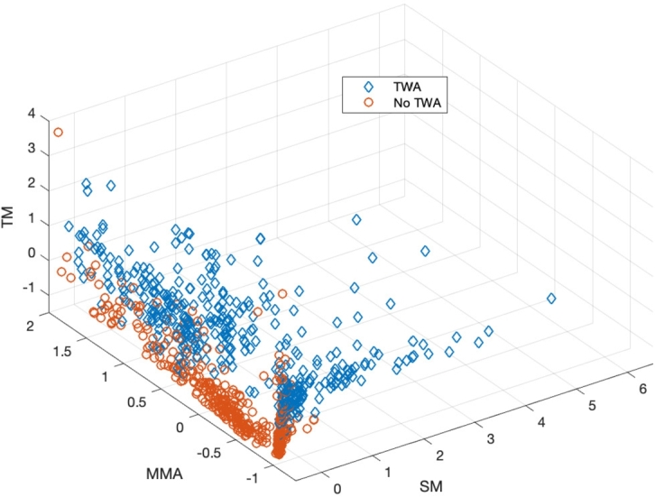
Input vectors for the ML algorithms. The normalized values from the TM, SM and MMA are represented in the Z, Y and X axis respectively.
4.2. Validation and test procedure
The procedure to evaluate the proposed models is carried out in two–steps. Five–fold CV is first achieved to perform hyperparameter tuning, as previously referred, followed by the test of the model on an independent set. Next, and because the test set has approximately the same size as that of the 5 folds, a permutation procedure of the test set is applied to analyze the robustness of the ML algorithms.
Fig. 3 depicts the strategy to perform hyperparameter tuning and to validate the results, relying on the patient group split described in Table 1. Model optimization is addressed by hyperparameter search through 5–fold CV, performed over patients from groups 1 up to 5 (PG1–PG5), each fold corresponding to a disjoint group of patients. The CV setting evaluates the performance of the model for the j–th hyperparameter tuple , resulting in the metrics , , obtained in the validation set of every fold, which is subsequently averaged throughout the five folds as follows (Eq. (10)):
| (10) |
The optimal model is obtained by choosing the tuple which optimizes the averaged metric (Eq. (11)):
| (11) |
Figure 3.

Cross Validation scheme of a model, where PG stands for Patient Group, kj refers to the hyperparameters tuple of a model, and ϕ stands for the metric utilized for the optimization problem. Patient group test set (PG6) is fitted with optimum hyperparameters obtained from CV. Notice that each PG corresponds to a disjoint group of patients.
The permutation scheme to analyze the robustness of the proposed models is depicted in Fig. 4 and works as follows. The strategy explained in Fig. 3 is iterated by choosing different patient groups as test set at each iteration. Thus, each permutation provides a different optimal model whose performance in estimated in different test sets. The global performance is given as the mean and the standard deviation, the latter to inform about the consistency of the trained model on different test sets.
Figure 4.

Diagram representation of permutation scheme, where PG stands for Patient Group. Notice that each PG corresponds to a disjoint group of patients.
Notice that the design of the ML models relies on an optimization process with regard to an overal metric ϕ, which can be chosen among several ones, such as the cost function. In this work, optimal models have been obtained using the accuracy score (defined in Eq. (12)) as the optimization metric.
4.3. Performance evaluation
Performance assessment is evaluated with the well known figures of merit used in the field, namely, Accuracy, Precision, Recall, and F1 score. Accuracy, calculated as in Eq. (12), stands for the probability of any ECG block be well classified:
| (12) |
where: TP stands for an alternans ECG block well classified (true positive); TN for a control ECG block well classified (true negative); FN for an alternans block classified as control (false negative); and FP for a control block classified as with TWA (false positive). Precision (Eq. (13)) assesses the probability of a detection being correct (positive predictivity):
| (13) |
and Recall (Eq. (14)) informs about the probability of an ECG block containing TWA be well classified (sensitivity):
| (14) |
F1 score, determined in Eq. (15), provides a joint measure in a single metric as a balance between the two previous ones:
| (15) |
Finally, a summary of the procedure followed in this Section is depicted in the flow chart of Fig. 5.
Figure 5.

Flow chart of ML setup followed in this work.
5. Results
The performance results are obtained as the mean and standard deviation of the different permutations represented in Fig. 4, where the model resulting from each patient group iteration is trained on the set employed to optimize it, and it is validated on the test set assigned to the permutation.
Every graph of Fig. 6 shows the performance of the different ML algorithms for one specific metric (from top to bottom, Accuracy, Precision, Recall, and F1 score). Each couple of bars stands for the mean value of the corresponding metric in the train test (bar on the left) and in the test set (bar on the right). The standard deviation is represented as whiskers around the mean. All the algorithms yield similar results. In general, the mean values of the metrics in the train set are very close to those of the test set, which indicates an appropriate generalization of the results. Nonetheless, the standard deviation in the test set is significantly higher than in the train set. The reason is twofold: On the one hand, it can be due to an insufficient count of test instances; on the other hand, the influence of inter–patient variability, which causes that the characteristics of the patients included in the test set are not fully learnt from patients of the train test.
Figure 6.

Classification performance for different ML algorithms in terms of mean and standard deviation. Every pair of bars stands for the metric value in the train (left) and test (right) sets.
In analyzing ML methods, a good choice should be one which holds some of the following properties. A small decrease in performance from train to test, indicating nice generalization capacity. Notice that a huge gap from train to test may be indicative of overfitting to the train set. Also a small standard deviation in the test set as an indicator of consistency, because this property suggests that different models (one ML algorithm with different hyperparameters) trained and tested on different datasets, perform similar to each other. The evaluation of Precision and Recall (second and third graphs from top to bottom) is also important because they report the rate of FP and FN, respectively, and a good method should provide a reasonable trade–off between these magnitudes. The results reported in the second column of Fig. 6, corresponding to Decision Tree, represent a good deal among the aforementioned points. Decision Tree is also the algorithm which yields better precision and recall in the test set.
Table 3 reports the performance of Decision Tree and the comparison with the SM when applied directly on every instance of the dataset. As can be seen, rather than using the SM alone, the use of learning methods to detect alternans increases the F1 score from 0.76 to 0.89. This improvement is due to a significant Recall upgrade at the expense of a small Precision decrease, resulting in a better balance among the two magnitudes. Basically, learning from data to identify alternans elicits a detection growth (TP increase) paying a small cost in the increment of the false alarm.
Table 3.
Mean and standard deviation performance of Decision Tree in the six permutations and comparison with the Spectral Method.
| Method | Set | Accuracy | Precision | Recall | F1 score |
|---|---|---|---|---|---|
| SM | All | 0.79 | 0.93 | 0.64 | 0.76 |
| Decision Tree | Train | 0.90 ± 0.01 | 0.89 ± 0.01 | 0.91 ± 0.01 | 0.90 ± 0.01 |
| Test | 0.88 ± 0.04 | 0.89 ± 0.05 | 0.90 ± 0.05 | 0.89 ± 0.03 | |
As depicted in Table 4, the results obtained for Decision Tree from CV in each permutation are stable, hence reaffirming the robustness of the classifier. The optimal hyperparameters Maximum Number of Splits and Minimum Leaf Size are shown for each permutation as well.
Table 4.
Results on the test set and optimal hyperparameters Maximum Number of Splits (MaxNumSplits) and MinLeafSize (Minimum Leaf Size) for the 6 permutations with Decision Trees.
| Perm 1 | Perm 2 | Perm 3 | Perm 4 | Perm 5 | Perm 6 | |
|---|---|---|---|---|---|---|
| Accuracy | 0,82 | 0,89 | 0,88 | 0,94 | 0,89 | 0,89 |
| Precision | 0,82 | 0,88 | 0,86 | 0,93 | 0,95 | 0,87 |
| Recall | 0,85 | 0,91 | 0,92 | 0,95 | 0,83 | 0,92 |
| F1 score | 0,83 | 0,89 | 0,89 | 0,94 | 0,89 | 0,89 |
| Optimal MaxNumSplits | 4 | 4 | 4 | 4 | 4 | 4 |
| Optimal MinLeafSize | 12 | 2 | 28 | 2 | 19 | 2 |
6. Discussion
One of the purposes of the current work was the development of an experimental setting to check the efficiency of learning–based algorithms for detection and estimation of TWA in surface ECG. The configuration of a database was essential to achieve this goal, because to date, there are no available recordings with labeled TWA to conduct supervised experiments. This is in fact the main constraint to report solutions in this field, so the methodology of the design of a database for TWA analysis proposed in this work can be considered as a contribution.
The procedure to assemble a set of data is carried out as an extension of a methodology previously introduced in preceding works [17], [19], [18], with the aim of covering as best as possible the actual ECG variability in both dimensions, namely, the structural variability of the signal, which represents the dynamic of the cardiac system, and the existing waveform difference among patients. Thus, the configuration of control ECGs, i.e., signals free from alternans, is obtained as a result of a two step evaluation of actual ECG recordings, which consists of first collecting ECGs with normal sinus rhythm followed by the selection of the signals resulting from a negative test of TWA. In this way, the posterior inclusion of TWA sections with alternant waves of different shape and scale (either with or without the addition of noise, as done in [17], [18]) enables the design of a diverse set of annotated datasets. The SM has been chosen for the selection of control signals because alternans identification with this method relies on an accepted decision criterion, something which is not clearly reported by other methods. The procedure to obtain a database is easy to replicate and the choice of signals from opensource banks ensures reproducibility, though notice that the final result in the database configuration may have small variations depending on the manner the different processing blocks are implemented, such is the case of the SM.
The experimental setting presented in this work constitutes a TWA detection experiment which operates on signal excerpts of 32–heartbeats long for the identification of a sustained alternant wave of 35 μV introduced in the entire segment. This is an initial attempt to demonstrate the liability of learning methods applied in this field, and as shown by the results, the inclusion of a classification stage to decide about the presence of TWA can outperform traditional techniques. Nevertheless, further studies must be accomplished so that the systems can learn from a wider variety of alternans configurations, namely, different and varying amplitudes throughout the segment, considering non–stationary TWA, i.e., non–sustained in the entire window, and including phase shift of the alternant pattern [47]. This research could be tackled further by following the framework proposed in this work, but for this purpose, a significant increase of the dataset must be addressed.
Another important advantage that an ML method can report in the field of TWA detection is to provide decision making solutions, because this issue is not well defined with most of the current existing methods. Regarding the SM, it provides a well defined and clinically accepted threshold for the K score, but as any other method relying on spectrum analysis, it requires quasi–stationary conditions of the signal, and it is typically applied to a middle–term window length of 128 heartbeats, while the performance decays for shorter windows. Thus, the SM is not a suitable technique to be used with ambulatory recordings, where a response must be supplied in a short–term dimension. On the other hand, the MMA and the TM estimate the alternant voltage, relying the decision on a cutpoint value. Nonetheless, the selection of reliable cutpoints to identify positive TWA is not an easy task [48], as it requires the development of clinical studies, something that has been possible with the MMA because it is implemented in commercial ECG devices. Thus, cutpoints for this method have been found, e.g., μV in patients during early post–myocardial infarction [36], [49] indicates severely elevated risk for sudden cardiac death. However, methodological studies comparing several methods have shown that the MMA may report false positive TWA due to the inherent T–wave variability, the influence of respiration in the ECG, as well as higher levels of noise and artifact contaminating the ECG [21], [22], [50], while others not.
The use of a more sophisticated signal model, with an extended database, will surely require the application of enhanced tools, designed by means of the incorporation of additional features to feed the classification systems. For the design of any TWA signal index, the attention must be drawn to the repolarization segment to extract the information concerning any every–other–beat transition of that part of the ECG. Because extracting this information is the objective of any TWA marker, such those introduced in Section 1, these indicators can be considered as very good parameters for ML algorithms based on feature extraction. Recently, the alternation of the whole heartbeat is raising interest as indicator of cardiac instability. Although P wave alternans does not occur frequently, it has been found to be a predictor of atrial fibrillation. Similarly, QRS alternans is patent in case of supraventricular and ventricular tachycardias [51], [52]. The underlying signal processing problem of heartbeat alternans is basically the same as that of the TWA, and it also suffers from the lack of gold standard. The current work could serve as an inspiration to tackle the alternans problem in the whole beat through the design of a specific signal model, the adaptation of TWA markers to the overall problem, and the use of existing indices for this purpose [52].
To date, we have not found previous works tackling TWA detection based on ML methods published in international indexed journals, but two conference papers [32], [33] reporting an F1 score of 89% and 95.9% respectively, with the Physionet TWA dataset [34], [53]. Although this database is of great value, it may not be appropriate for ML methods since it contains different segments from the same patients, and they are unidentified. Therefore, patient separation is impossible in the test and train sets, avoiding the evaluation of the effect that intra–patient overfitting can cause. Furthermore, the limitation of this database is the lack of labels specifying the information related to TWA in specific regions of the ECG, which has hardly encouraged the development of novel TWA studies with this tool.
Some parts of this section deal with future works related to traditional ML algorithms because there are still much work to do. Nonetheless, research on detection of TWA relying on Deep Learning should also be tackled because these networks have proven nice performance as outstanding approaches within the family of representation learning. Nonetheless, the exploding amount of parameters that this type of algorithms needs to adjust will surely require to enlarge the database by scrutinizing more data, e.g., by following a similar methodology than that proposed here. Because this approach is not sufficient, the challenge of annotating TWA on real ECG becomes more evident, being one of the biggest challenges to be tackled in this field. Manually annotation is in general cumbersome, and particularly in this area, where TWA is not straightforward visible on the ECG, requiring previous signal processing and special help for visualization. For this purpose, techniques such as Active Learning could be used by combining labeling and the use of trained models to track TWA on real data to increase the amount of labeled data and, at the same time, improving the performance of the detection algorithms [54]. Although Deep Neural Network, is usually applied to the raw ECG, the entire heartbeat, or a transformed version of them, processing the whole beat in TWA could elicit false alarm as long as other types of alternans could be detected. Likely in the initial attempts with Convolutional Neural Networks, matrix M from Eq. (1) could be a suitable choice.
7. Conclusion
The experimental setting designed in this work to conduct supervised experiments for TWA detection constitutes a contribution to further investigations with ML and DL algorithms. The ensemble TWA detection method proposed in this work, based on ML algorithms fed with features that are the results of three traditional TWA detection and estimation methods, outperformed the SM used as a gold standard. Learning from data to identify alternans elicits a substantial detection growth at the expense of a small increment of the false alarm.
Author contributions statement
RGE, MGFC, and MBV conceived, designed, and performed the experiments. All coauthors analyzed and interpreted the data, contributed reagents, materials, analysis tools or data, and also all coauthors wrote the paper.
Funding statement
This work has been partially supported under project EPU-INV/2020/002 from Community of Madrid and University of Alcalá.
Declaration of Competing Interest
The authors declare no conflict of interest.
Contributor Information
Miriam Gutiérrez Fernández–Calvillo, Email: miriam.gutierrez@urjc.es.
Rebeca Goya–Esteban, Email: rebeca.goyaesteban@urjc.es.
Fernando Cruz–Roldán, Email: fernando.cruz@uah.es.
Antonio Hernández–Madrid, Email: antonio.hernandez@uah.es.
Manuel Blanco–Velasco, Email: manuel.blanco@uah.es.
Data availability
Data available on request from the authors.
References
- 1.Smith J.M., Clancy E.A., Valeri C.R., Ruskin J.N., Cohen R.J. Electrical alternans and cardiac electrical instability. Circulation. 1988;77(1):110–121. doi: 10.1161/01.cir.77.1.110. [DOI] [PubMed] [Google Scholar]
- 2.Rosenbaum D.S., Albrecht P., Smith J.M., Garan H., Ruskin J.N., Cohen R.J. Electrical alternans and vulnerability to ventricular arrhythmias. N. Engl. J. Med. 1994;330(4):235–241. doi: 10.1056/NEJM199401273300402. [DOI] [PubMed] [Google Scholar]
- 3.Gimeno-Blanes F.J., Blanco-Velasco M., Barquero-Pérez O., García-Alberola A., Rojo-Álvarez J.L. Sudden cardiac risk stratification with electrocardiographic indices - a review on computational processing, technology transfer, and scientific evidence. Front. Physiol. 2016;7(82) doi: 10.3389/fphys.2016.00082. [DOI] [PMC free article] [PubMed] [Google Scholar]
- 4.Gehi A.K., Stein R.H., Metz L.D., Gomes J.A. Microvolt T–wave alternans for the risk stratification of ventricular tachyarrithmic events. J. Am. Coll. Cardiol. 2005;46(1):75–82. doi: 10.1016/j.jacc.2005.03.059. [DOI] [PubMed] [Google Scholar]
- 5.Merchant F.M., Sayadi O., Moazzami K., Puppala D., Armoundas A.A. T-wave alternans as an arrhythmic risk stratifier: state of the art. Curr. Cardiol. Rep. 2013;15(9):1–9. doi: 10.1007/s11886-013-0398-7. [DOI] [PMC free article] [PubMed] [Google Scholar]
- 6.Nearing B.D., Huang A.H., Verrier R.L. Dynamic tracking of cardiac vulnerability by complex demodulation of the T wave. Science. 1991;252(5004):437–440. doi: 10.1126/science.2017682. [DOI] [PubMed] [Google Scholar]
- 7.Burattini L., Zareba W., Moss A.J. Correlation method for detection of transient T-wave alternans in digital holter ECG recordings. Ann. Noninvasive Electrocardiol. 1999;4(4):416–424. [Google Scholar]
- 8.Nearing B.D., Verrier R.L. Modified moving average analysis of T-wave alternans to predict ventricular fibrillation with high accuracy. J. Appl. Physiol. 2002;92(2):541–549. doi: 10.1152/japplphysiol.00592.2001. [DOI] [PubMed] [Google Scholar]
- 9.Martínez J.P., Olmos S. Methodological principles of T wave alternans analysis: a unified framework. IEEE Trans. Biomed. Eng. 2005;52(4):599–613. doi: 10.1109/TBME.2005.844025. [DOI] [PubMed] [Google Scholar]
- 10.Monasterio V., Clifford G., Laguna P., Martínez J.P. A multilead scheme based on periodic component analysis for T-wave alternans analysis in the ECG. Ann. Biomed. Eng. 2010;38(8):2532–2541. doi: 10.1007/s10439-010-0029-z. [DOI] [PubMed] [Google Scholar]
- 11.Burattini L., Zareba W., Burattini R. Adaptive match filter based method for time vs. amplitude characterization of microvolt ECG T-wave alternans. Ann. Biomed. Eng. 2008;36(9):1558–1564. doi: 10.1007/s10439-008-9528-6. [DOI] [PubMed] [Google Scholar]
- 12.Bashir S., Bakhshi A.D., Maud M.A. A template matched-filter based scheme for detection and estimation of T-wave alternans. Biomed. Signal Process. Control. 2014;13:247–261. [Google Scholar]
- 13.Romero I., Grubb N., Clegg G., Robertson C., Addison P., Watson J. T-wave alternans found in preventricular tachyarrhythmias in CCU patients using a wavelet transform-based methodology. IEEE Trans. Biomed. Eng. 2008;55(11):2658–2665. doi: 10.1109/TBME.2008.923912. [DOI] [PubMed] [Google Scholar]
- 14.Ghoraani B., Krishnan S., Selvaraj R.J., Chauhan V.S. T wave alternans evaluation using adaptive time–frequency signal analysis and non-negative matrix factorization. Med. Eng. Phys. 2011;33(6):700–711. doi: 10.1016/j.medengphy.2011.01.007. [DOI] [PubMed] [Google Scholar]
- 15.Nemati S., Abdala O., Monasterio V., Yim-Yeh S., Malhotra A., Clifford G.D. A nonparametric surrogate-based test of significance for T-wave alternans detection. IEEE Trans. Biomed. Eng. 2011;58(5):1356–1364. doi: 10.1109/TBME.2010.2047859. [DOI] [PMC free article] [PubMed] [Google Scholar]
- 16.Monasterio V., Laguna P., Martínez J.P. Multilead analysis of T-wave alternans in the ECG using principal component analysis. IEEE Trans. Biomed. Eng. 2009;56(7):1880–1890. doi: 10.1109/TBME.2009.2015935. [DOI] [PubMed] [Google Scholar]
- 17.Blanco-Velasco M., Cruz-Roldán F., Godino-Llorente J.I., Barner K.E. Nonlinear trend estimation of the ventricular repolarization segment for T–wave alternans detection. IEEE Trans. Biomed. Eng. 2010;57(10):2402–2412. doi: 10.1109/TBME.2010.2048109. [DOI] [PubMed] [Google Scholar]
- 18.Blanco-Velasco M., Goya-Esteban R., Cruz-Roldán F., García-Alberola A., Rojo-Álvarez J.L. Benchmarking of a T–wave alternans detection method based on empirical mode decomposition. Comput. Methods Programs Biomed. 2017;145:147–155. doi: 10.1016/j.cmpb.2017.04.005. [DOI] [PubMed] [Google Scholar]
- 19.Goya-Esteban R., Barquero-Pérez O., Blanco-Velasco M., Caamaño-Fernández A., García-Alberola A., Rojo-Álvarez J. Nonparametric signal processing validation in T–wave alternans detection and estimation. IEEE Trans. Biomed. Eng. 2014;61(4):1328–1338. doi: 10.1109/TBME.2014.2304565. [DOI] [PubMed] [Google Scholar]
- 20.Cuesta-Frau D., Micó-Tormos P., Aboy M., Biagetti M.O., Austin D., Quinteiro R.A. Enhanced modified moving average analysis of T–wave alternans using a curve matching method: a simulation study. Med. Biol. Eng. Comput. 2009;47(3):323–331. doi: 10.1007/s11517-008-0415-y. [DOI] [PubMed] [Google Scholar]
- 21.Burattini L., Bini S., Burattini R. Comparative analysis of methods for automatic detection and quantification of microvolt T-wave alternans. Med. Eng. Phys. 2009;31(10):1290–1298. doi: 10.1016/j.medengphy.2009.08.009. [DOI] [PubMed] [Google Scholar]
- 22.Burattini L., Bini S., Burattini R. Correlation method versus enhanced modified moving average method for automatic detection of T–wave alternans. Comput. Methods Programs Biomed. 2010;98(1):94–102. doi: 10.1016/j.cmpb.2010.01.008. [DOI] [PubMed] [Google Scholar]
- 23.Janusek D., Kania M., Zaczek R., Zavala-Fernandez H., Maniewski R. A simulation of T–wave alternans vectocardiographic representation performed by changing the ventricular heart cells action potential duration. Comput. Methods Programs Biomed. 2014;114(1):102–108. doi: 10.1016/j.cmpb.2014.01.015. [DOI] [PubMed] [Google Scholar]
- 24.Jiang J., Zhang H., Pi D., Dai C. A novel multi-module neural network system for imbalanced heartbeats classification. Expert Syst. Appl. 2019;X 1 [Google Scholar]
- 25.Radhakrishnan T., Karhade J., Ghosh S., Muduli P., Tripathy R., Acharya U.R. AFCNNet: automated detection of AF using chirplet transform and deep convolutional bidirectional long short term memory network with ECG signals. Comput. Biol. Med. 2021;137 doi: 10.1016/j.compbiomed.2021.104783. [DOI] [PubMed] [Google Scholar]
- 26.Yang Q., Zou L., Wei K., Liu G. Obstructive sleep apnea detection from single-lead electrocardiogram signals using one-dimensional squeeze-and-excitation residual group network. Comput. Biol. Med. 2022;140 doi: 10.1016/j.compbiomed.2021.105124. [DOI] [PubMed] [Google Scholar]
- 27.Wang T., Lu C., Sun Y., Yang M., Liu C., Ou C. Automatic ECG classification using continuous wavelet transform and convolutional neural network. Entropy. 2021;23(1):119. doi: 10.3390/e23010119. [DOI] [PMC free article] [PubMed] [Google Scholar]
- 28.Liu X., Wang H., Li Z., Qin L. Deep learning in ECG diagnosis: a review. Knowl.-Based Syst. 2021;227 [Google Scholar]
- 29.Xue J., Yu L. Applications of machine learning in ambulatory ECG. Hearts. 2021;2(4):472–494. [Google Scholar]
- 30.Sun J.-Y., Shen H., Qu Q., Sun W., Kong X.-Q. The application of deep learning in electrocardiogram: where we came from and where we should go? Int. J. Cardiol. 2021;337:71–78. doi: 10.1016/j.ijcard.2021.05.017. [DOI] [PubMed] [Google Scholar]
- 31.Mincholé A., Camps J., Lyon A., Rodríguez B. Machine learning in the electrocardiogram. J. Electrocardiol. 2019;57:S61–S64. doi: 10.1016/j.jelectrocard.2019.08.008. [DOI] [PubMed] [Google Scholar]
- 32.Karnaukh O., Karplyuk Y., Nikitiuk N. IEEE 38th International Conference on Electronics and Nanotechnology. 2018. Evaluation of machine learning techniques for ECG T–wave alternans; pp. 346–350. [Google Scholar]
- 33.Karnaukh O., Karplyuk Y. IEEE 40th International Conference on Electronics and Nanotechnology. 2020. Application of machine learning methods for artificial ECG with T–wave alternans; pp. 613–617. [Google Scholar]
- 34.Goldberger A.L., Amaral L.A.N., Glass L., Hausdorff J.M., Ivanov P.C., Mark R.G., Mietus J.E., Moody G.B., Peng C.-K., Stanley H.E. PhysioBank, PhysioToolkit, and PhysioNet: components of a new research resource for complex physiologic signals. Circulation. 2000;101(23):215–220. doi: 10.1161/01.cir.101.23.e215. [DOI] [PubMed] [Google Scholar]
- 35.Martínez J.P., Olmos S., Wagner G., Laguna P. Characterization of repolarization alternans during ischemia: time-course and spatial analysis. IEEE Trans. Biomed. Eng. 2006;53(4):701–711. doi: 10.1109/TBME.2006.870233. [DOI] [PubMed] [Google Scholar]
- 36.Verrier R.L., Klingenheben T., Malik M., El-Sherif N., Exner D.V., Hohnloser S.H., Ikeda T., Martínez J.P., Narayan S.M., Nieminen T., Rosenbaum D.S. Microvolt T–wave alternans: physiological basis, methods of measurement, and clinical utility—consensus guideline by international society for holter and noninvasive electrocardiology. J. Am. Coll. Cardiol. 2011;58(13):1309–1324. doi: 10.1016/j.jacc.2011.06.029. [DOI] [PMC free article] [PubMed] [Google Scholar]
- 37.Rosenbaum D.S., Jackson L.E., Cohen R.J. Predicting sudden cardiac death from T wave alternans of the surface electrocardiogram: promise and pitfalls. J. Cardiovasc. Electrophysiol. 1996;7(11):1095–1111. doi: 10.1111/j.1540-8167.1996.tb00487.x. [DOI] [PubMed] [Google Scholar]
- 38.Verrier R.L., Nearing B.D., la Rovere M.T., Pinna G.D., Mittleman M.A., Bigger J.T., Schwartz P.J. Ambulatory electrocardiogram–based tracking of T wave alternans in postmyocardial infarction patients to assess risk of cardiac arrest of arrhythmic death. J. Cardiovasc. Electrophysiol. 2003;14:705–711. doi: 10.1046/j.1540-8167.2003.03118.x. [DOI] [PubMed] [Google Scholar]
- 39.Bishop C.M. Springer-Verlag; 2006. Pattern Recognition and Machine Learning. (Information Science and Statistics). [Google Scholar]
- 40.Hastie T., Tibshirani R., Friedman J. 2nd edition. Springer; 2009. The Elements of Statistical Learning: Data Mining, Inference and Prediction. [Google Scholar]
- 41.Breiman L. Random forests. Mach. Learn. 2001;45(1):5–32. [Google Scholar]
- 42.Wu X., Kumar V., Quinlan J. Ross, Ghosh J., Yang Q., Motoda H., McLachlan G.J., Ng A., Liu B., Yu P.S., et al. Top 10 algorithms in data mining. Knowl. Inf. Syst. 2008;14(1):1–37. [Google Scholar]
- 43.Riedmiller M., Braun H. IEEE International Conference on Neural Networks. IEEE; 1993. A direct adaptive method for faster backpropagation learning: the RPROP algorithm; pp. 586–591. [Google Scholar]
- 44.Goodfellow I., Bengio Y., Courville A. MIT Press; 2016. Deep Learning. [Google Scholar]
- 45.Moody G., Mark R. The impact of the MIT-BIH arrhythmia database. IEEE Eng. Med. Biol. Mag. 2001;20(3):45–50. doi: 10.1109/51.932724. [DOI] [PubMed] [Google Scholar]
- 46.Taddei A., Distante G., Emdin M., Pisani P., Moody G.B., Zeelenberg C., Marchesi C. The European ST-T database: standard for evaluating systems for the analysis of ST-T changes in ambulatory electrocardiography. Eur. Heart J. 1992;13(9):1164–1172. doi: 10.1093/oxfordjournals.eurheartj.a060332. [DOI] [PubMed] [Google Scholar]
- 47.Martín-Yebra A., Monasterio V., Cygankiewicz I., Bayés-de Luna A., Caiani E.G., Laguna P., Martínez J.P. Post-ventricular premature contraction phase correction improves the predictive value of average T-wave alternans in ambulatory ECG recordings. IEEE Trans. Biomed. Eng. 2018;65(3):635–644. doi: 10.1109/TBME.2017.2711645. [DOI] [PubMed] [Google Scholar]
- 48.Hohnloser S.H. Risk stratification using T–wave alternans: more questions waiting to be answered. J. Cardiovasc. Electrophysiol. 2008;19(10):1043–1044. doi: 10.1111/j.1540-8167.2008.01205.x. [DOI] [PubMed] [Google Scholar]
- 49.Verrier R.L. Modified moving average T-wave alternans cutpoints. Indian Pacing and Electrophysiol. J. 2021;21(2):139. doi: 10.1016/j.ipej.2021.01.009. [DOI] [PMC free article] [PubMed] [Google Scholar]
- 50.Wan X., Li Y., Xia C., Wu M., Liang J., Wang N. A T-wave alternans assessment method based on least squares curve fitting technique. Measurement. 2016;86:93–100. [Google Scholar]
- 51.Marcantoni I., Calabrese D., Chiriatti G., Melchionda R., Pambianco B., Rafaiani G., Scardecchia E., Sbrollini A., Morettini M., Burattini L. In: XV Mediterranean Conference on Medical and Biological Engineering and Computing – MEDICON 2019. Henriques J., Neves N., de Carvalho P., editors. Springer International Publishing; 2020. Electrocardiographic alternans: a new approach; pp. 159–166. [Google Scholar]
- 52.Marcantoni I., Sbrollini A., Morettini M., Swenne C.A., Burattini L. Enhanced adaptive matched filter for automated identification and measurement of electrocardiographic alternans. Biomed. Signal Process. Control. 2021;68 [Google Scholar]
- 53.Moody G. 2008 Computers in Cardiology. IEEE; 2008. The physionet/computers in cardiology challenge 2008: T-wave alternans; pp. 505–508. [DOI] [PMC free article] [PubMed] [Google Scholar]
- 54.Ahsan M.A., Qayyum A., Razi A., Qadir J. An active learning method for diabetic retinopathy classification with uncertainty quantification. Med. Biol. Eng. Comput. 2022;60(10):2797–2811. doi: 10.1007/s11517-022-02633-w. [DOI] [PubMed] [Google Scholar]
Associated Data
This section collects any data citations, data availability statements, or supplementary materials included in this article.
Data Availability Statement
Data available on request from the authors.