Efficient representations of binarized health deficit data: the frailty index and beyond

Abstract

We investigated efficient representations of binarized health deficit data using the 2001–2002 National Health and Nutrition Examination Survey (NHANES). We compared the abilities of features to compress health deficit data and to predict adverse outcomes. We used principal component analysis (PCA) and several other dimensionality reduction techniques, together with several varieties of the frailty index (FI). We observed that the FI approximates the first — primary — component obtained by PCA and other compression techniques. Most adverse outcomes were well predicted using only the FI. While the FI is therefore a useful technique for compressing binary deficits into a single variable, additional dimensions were needed for high-fidelity compression of health deficit data. Moreover, some outcomes — including inflammation and metabolic dysfunction — showed high-dimensional behaviour. We generally found that clinical data were easier to compress than lab data. Our results help to explain the success of the FI as a simple dimensionality reduction technique for binary health data. We demonstrate how PCA extends the FI, providing additional health information, and allows us to explore system dimensionality and complexity. PCA is a promising tool for determining and exploring collective health features from collections of binarized biomarkers.

Supplementary Information

The online version contains supplementary material available at 10.1007/s11357-022-00723-z.

Introduction

Biological dysfunction arising from damage is central to aging [1]. Representing dysfunction requires robust summary measures of aging data, which can then help us to operationalize theories of causal mechanisms [1–3]. Is there a systematic way to generate summary measures from observed health deficits? How well do they predict a battery of adverse outcomes?

The frailty index (FI, see Table 1 for key abbreviations) is a simple, robust measure that is strongly predictive of general adverse outcomes [4, 5]. Dichotomizing data as healthy (0) or deficit (1) probes dysfunction directly. The FI is defined as the average number of dysfunctional (deficit) health variables an individual has [6]. Conventionally, the FI is constructed from self-reported questionnaire — “clinical” — data, such as (instrumental) activities of daily living (I)ADLs and physical limitations. Recently, the FI has been extended to include “lab” biomarker data [7, 8].

Table 1.

Nomenclature

FI	Frailty index
FP	Frailty phenotype
(I)ADL	(Instrumental) activities of daily living
PC(A)	Principal component (analysis)
LPC(A)	Logistic PC (analysis)a
LSV(D)	Logistic singular value (decomposition)b
GLM	Generalized linear model

^a Cousin of PCA

^b Cousin of LPCA

Aging is widely considered to be multidimensional [1–3, 9–11]. The FI is just one of many univariate summary health measures. In particular, many “biological ages” have been proposed. These measures overlap only moderately, implying that a complete description of “biological age” would require several of them [12, 13]. Machine learning studies also suggest multiple dimensions of health information, though survival information appears to compress into just one or two dimensions [14]. Furthermore, interventional study reviews often report improvement along one dimension at the expense of worsening along other dimensions: for example, mice treated with metformin show improved treadmill performance but reduced visual acuity [15]. For which outcomes is a univariate health measure sufficient? Do integrative hallmarks of aging [1] or bow tie systems [16], which mediate interactions between multiple systems, require multidimensional health measures?

The rapidly increasing dimensionality of “omics” aging data [17] makes these questions pressing. For example, Jansen et al. [12] studied over 20,000 gene expressions from fewer than 3000 individuals. Data with more variables than individuals carry the “curse of dimensionality” which can lead to overfitting and loss of interpretability with standard algorithms [18]. Condensing high-dimensional data into a few salient features simplifies statistical modelling [18, 19]. To achieve this, we need scalable and robust dimensionality reduction techniques.

While the FI is a simple and reproducible dimensionality reduction technique [20] that compresses 30+ binary health variables [6] into a single, graded measure [21], it has not been systematically extended to higher-dimensional health features. Ad hoc multivariate extensions such as domain-specific FIs [22, 23] or multiple biological ages [13] neglect the possibilities that these measures may have gaps or redundancies in the information they contain.

The canonical dimensionality reduction technique in machine learning and statistics is principal component analysis (PCA), which is robust, fast, and systematically extensible [18]. PCA linearly combines (rotates) existing health variables into a complete set of new “latent” health variables — principal components (PCs) — ordered from most to least variance. By construction, the PCs are mutually independent and hence do not suffer the problem of redundant information faced by multiple ad hoc approaches.

PCA has been used to improve epigenetic clock reliability [24], and to analyse raw biomarker data [25, 26] and dysfunction biomarkers [27]. PCA is robust to covariates, including sex, race, and study population [25]. When used correctly, PCA summarizes the salient information in a dataset. For example, Entwistle et al. [28] applied PCA to NHANES III dietary data and identified the first 4 PCs as being idealized dietary patterns. Nevertheless, studies using PCA to generate new health measures (PCs) from deficit data are rare. Few, if any, have leveraged the extensive literature on health deficit data that surrounds the FI. Furthermore, none of the aforementioned studies has systematically explored multiple dimensionality reduction algorithms nor the effect of modifying the number of PCs on adverse outcome prediction. What are the generic features of dimensionality reduction of health deficit data? How can this help us to understand and build upon the success of the FI?

We should also explore what is the correct number of PCs to use for health deficit data. Arbitrarily restricting which PCs to use has led to serious criticisms of its reproducibility for low-rank projections (e.g. only using the first two PCs) [29]. Others have noted that mortality information can be found in low-variance PCs, which are often neglected [24].

While the FI and PCA are both linear transformations, the FI imposes equal weightings of each variable whereas PCA does not. Accordingly, the FI and PCA need not be related. Nevertheless, previous work has shown that the first PC of biomarker dysfunction data from hemodialysis patients approximately reproduces the two key phenomenon of the FI: approximately equal weightings across input variables, and good prediction of adverse outcomes, including the frailty phenotype (FP) [27]. Furthermore, the FI has been shown to efficiently compress clinical, deficit questionnaire data, with little unexplained residual variance [30]. However, research on biomarker lab deficit data implies the presence of additional dimensions [31]. How many dimensions are relevant in lab biomarker data, and do they overlap with clinical dimensions? Any such information that is shared between lab and clinical domains will affect joint dimensionality reduction.

As with the FI, our primary interest is in damage arising from dysfunction, so we binarize data as either normal (0) or dysfunctional/deficit (1). We expect that compression of health deficit data will find efficient representations of both dysfunction and adverse outcomes because health deficits are themselves adverse outcomes, e.g. ADLs [32]. This improves interpretability — dysfunction is what we care about — and saves us from issues endemic to continuous variables, such as scaling, healthy variability, and non-normal behaviour. Recent advances in PCA specific to binary data provide additional techniques that we also explore: “logistic” PCA [33] and “logistic SVD” [33, 34] (SVD: singular value decomposition).

All of these PCA algorithms are lightweight with minimal assumptions. They compress data into efficient rank-ordered representations, where the first dimension contains the most information and the last contains the least. In contrast, latent variable models such as grade of membership [35–37], while more directly interpretable, have sub-optimal compression efficiency and do not rank-order their latent space. Efficient, rank-ordered representations will effectively coarse grain the data, allowing us to answer our questions about dimensionality and information flow. Here, we restrict our attention to PCA and its variants.

The goal of this study is to systematically explore the use of PCA in compression and prediction of multidimensional health deficit data, and to compare PCA with the FI. We also examine PCA alternatives. Compression can tell us the maximum number of dimensions required to efficiently represent input data, but cannot a priori distinguish between useful information and noise. We compare compression of binary deficit data and prediction of adverse outcomes using both outcome associations and a generalized linear model (GLM). We include a battery of adverse outcomes to test predictive power. Finally, we take a deeper look at PCA, fully exploring its utility, its robustness, the patterns it extracts from the data, i.e. PCs, and its systematic mode of action. We demonstrate that PCA provides a multidimensional perspective of health not available to univariate health measures.

Methods

Figure 1 outlines the study pipeline. We split the data into three parallel analyses: compression, associations with input/outcome variables, and prediction using GLMs. We compared compression using the FI, PCA, logistic PCA (LPCA) [33], and logistic singular value decomposition (LSVD) [33, 34].

Fig. 1.

Study pipeline. We performed three parallel analyses: compression, feature associations, and outcome modelling. Data were preprocessed, resulting in an input matrix of health deficit data, X, and an outcome matrix of adverse outcomes, Y (rows: individuals, columns: variables). The input was transformed by a dimensionality reduction algorithm, represented by Φ, which was either the FI (frailty index), PCA (principal component analysis), LPCA (logistic PCA), or LSVD (logistic singular value decomposition). Each algorithm, Φ, generated a matrix of latent features with tunable dimension, Z (dimension: number of columns/features; the FI was not tunable). We tuned the size of this latent feature space, Z, to infer compression efficiency and the maximum dimensions of Z before features became redundant (binarizing with optimal threshold, η). The latent features were then associated with input and outcomes to infer their information content and the flow of information from input to output. The dimension of Z was then again tuned to predict the adverse outcomes. $Ŷ$ represents the outcome estimates by the generalized linear model (GLM), which were compared to ground truth, Y, to determine the minimum dimension of Z needed to achieve optimal prediction performance for each outcome. This procedure allowed us to characterize the flow of information through each dimensionality reduction algorithm

Data and pre-processing

We used data from the 2001–2002 NHANES with linked public mortality records [38]. We included individuals over age 60 (N = 1872) to focus on older individuals and to avoid problems with gated variables [39]. We used lab and clinical health deficit data from multiple domains to predict multiscale, multidomain outcomes. In total, we included 26 clinical predictors, 29 lab predictors, 47 outcomes, and 7 demographical variables.

The complete list of predictors, outcomes, and covariates is provided in Online Resource S1.1. We binarized all predictors using standard rules [40] (Tables S1 and S2). This simplified our analysis and forced our dimensionality reduction algorithms to find efficient representations of dysfunction — as desired. Outcomes included health biomarkers, disability, morbidity, and mortality. All continuous outcomes were standardized to zero mean and unit variance. We included 7 demographic covariates: age (top-coded at 85), and (binarized) sex, race, family income, education level, smoker status, and partner status.

The FI was computed as the average of binarized predictor variables [6]. The FP was included as an alternative frailty measure, defined as 3+ out of 5: low BMI, bottom 20% for gait speed (sex-adjusted), and self-reported: weakness, exhaustion, and low physical activity [41].

Imputation was performed using multivariate imputation by chained equations (MICE) version 3.10.0 [42]. We used the classification and regression tree (CART) method, which performs well with similar NHANES data [39]. We imputed all data, including predictors, outcomes, covariates, survival information, and auxiliary variables. Imputing outcomes had no significant effect on prediction accuracies: except for gait, which had a higher R² by $\sim 0.05$ (Online Resource S1.2.4). We imputed 15 times, reflecting the $\sim 15\%$ missingness [43]. We propagated the uncertainty in these imputations into our final results using Rubin’s rules [43]. We symmetrized and scaled standard errors (assuming normality), applied Rubin’s rules, then rescaled to 95% confidence intervals (CIs).

In Online Resource S1.2, we provide consistency checks on the imputed values and characterized the missing data. Individuals with missing data were older, with median (IQR) age 71 (65–78) vs 76 (67–83) (Wilcox p = 2 ⋅ 10^− 16), and had significantly worse survival, hazard ratio: 1.6(1) (p: 7 ⋅ 10^− 13, log-rank test). This means that the missing data were not missing completely at random and that failure to impute could lead to biased results [44]. We performed our initial analysis using complete case predictor and demographic data (no missingness for each individual), and available case outcome data (individuals were included for any outcome they had reported). Complete case analysis yielded similar results to our full, imputed analysis (Online Resource S4).

Performance metrics

Most of the binary outcomes and predictors were rare, with many occurring in less than 10% of study participants (Table S4). Such unbalanced data poses a problem when measuring binary performance [45]. An uninformative diagnostic test that returns negative regardless of disease status would have 90% accuracy in diagnosing a disease with 10% prevalence. Its Youden index [46], however, would be 0:

$$\text{Youden index}\equiv \text{sensitivity}+\text{specificity}-1.$$ 1

A perfectly informative test would have a Youden index of 1. The Youden index is strongly correlated with the AUC, which estimates the probability that a metric will correctly rank the positive individuals as higher than negative individuals [39]. Assuming case and control are both normality distributed with the same variance, the AUC and Youden index are redundant, for example Youden indexes of 0.2, 0.4, 0.6, and 0.8 correspond to AUCs of 0.64, 0.77, 0.88, and 0.97, respectively [47]; this model fits our data very well (Fig. S15).

When comparing continuous-continuous variable pairs we used Spearman’s ρ, a non-parametric measure of correlation [48]; we took the absolute value and estimated the confidence interval using quantiles from bootstrapping (with 2000 resamples). For models predicting continuous outcomes, we used R², the coefficient of determination, which measures the explained variance as a proportion of the total variance with 1 being perfect. The mean-squared error (MSE) is the average of the squared model residual [18]. We standardized continuous outcomes to zero mean and unit variance; hence, useful models have MSE < 1 (assuming unit variance, R² = 1 −MSE). Time-to-event outcomes, i.e. survival, were scored using the concordance-index (C-index), a cousin of the AUC [39]. GLM predictive power used R², MSE, AUC, Youden and/or the C-index. Outcome associations used Spearman’s ρ (specifically $|\rho |$), AUC, Youden, or the C-index (specifically $|C-0.5|$). Feature importance was first inferred from stepwise regression, then validated using selection frequency (Online Resource S3.3).

Input compression

We applied the FI, PCA, LPCA, and LSVD to the predictor variables (binarized lab and clinical data) — Fig. 2 illustrates how PCA compressed the data by decomposing the 2D joint deficit histogram. We treated the binary scale as an absolute scale for dysfunction, akin to the FI, so we did not center variables by their respective means. Lab and clinical data were compressed together and separately. Compression performance was measured by reconstruction accuracy. Data were compressed into a latent space using one of the four algorithms, then mapped back to the inputs using the inverse transform [33] (excluding the FI, which is not invertible). An ROC curve was then trained to map from the reconstruction (PCA, LPCA, and LSVD) or latent space (FI) to the inputs, providing an optimal cutting point to reconstruct the original inputs; this step calibrates the reconstruction. Test inputs were then compared to their reconstructions using the Youden index. Note that the Youden index is a (relatively) neutral measure that does not favour PCA, which minimizes the MSE, nor LPCA/LSVD, which minimize the Bernoulli deviance. We progressively increased the size of the latent space to be able to infer the minimum number of dimensions required for high-fidelity reconstruction. This yielded compression plots of increasing fidelity with increasing latent space dimension.

Fig. 2.

Principal component analysis (PCA) of binary data is equivalent to eigen-decomposing the 2D joint deficit histogram. The first column is the complete histogram, and the remaining columns sum to the first column (Eq. A6). The first PC is clearly dominant and is dense, meaning it is nearly equal weights for each variable (akin to the FI). The eigen-decomposition naturally finds blocks of correlated variables. When it runs out of blocks, it looks for strong diagonal terms. This causes PCA to naturally block out like-variables, e.g. lab vs clinical in PC2, similar to an expert choosing to create an FI out of variables from the same domain. Values have been transformed for visualization using sign(x)|x|^γ, γ = 2/3, see Fig. S16 for the figure without scaling

Generalized linear models (GLMs)

The primary motivation for using a regression model is to capture conditional effects, including demographical variables and the combined performance of multiple features. We used GLMs [48]. GLMs include linear, logistic, and Cox proportional hazard regression [18], allowing us to model each outcome variable with a homologous linear model.

We performed stepwise regression to analyse the effect of iteratively adding variables on the predictive performance, starting with the model that used only demographical information. Our motivation was to determine the optimal number of latent features to include in our models, which are naturally ordered by the dimensionality reduction algorithm, PC1 through to PC55. Stepwise models produced incremental prediction plots for comparison to the compression plots.

We inferred feature importance by building complete models that potentially included all predictors. Feature selection was performed using an L1-penalized GLM (LASSO), with the penalty selected using 10-fold cross-validation to pick the minimum mean-squared error (continuous outcomes) or deviance (binary outcomes) [49]. An L1-penalty penalizes regression coefficients that differ from 0, encouraging the model to retain only the most important features. Selection frequency was used as a measure of feature importance.

GLMs used to predict binary outcomes are known to underestimate the frequency of rare events, even for datasets with 1000s of individuals (such as ours) [45]. In Online Resource S2.1, we studied the use of observation weights to improve the Youden index. We found that the optimal weight of the i th individual was,

$$w_i=\left\{\begin{array}{cc}\frac{\text{Frequency of majority class}}{\text{Frequency of minority class}},& \text{if}i\text{is in minority}\mathrm{.}\\ 1,& \text{if}i\text{is in the majority}\mathrm{.}\end{array}\right)$$

This choice of weights is equivalent to the “weighted exogenous sampling” method [45], where we have weighted as if the population underlying the sample is perfectly balanced.

All computations were performed using R version 4.0.1 [48]. Error bars are standard errors unless specified otherwise. Errors are reported in parentheses, e.g. 12(3) ≡ 12 ± 3. Confidence intervals are 95%. We report out-of-sample performance metrics using 10-fold cross-validation for all parametric models, including compression and prediction. Out-of-sample means that the compression or prediction algorithm is completely ignorant of the testing data. This procedure estimates the expected performance on new, unseen data, from the same population, independent of the training set [50].

Results

Input compression

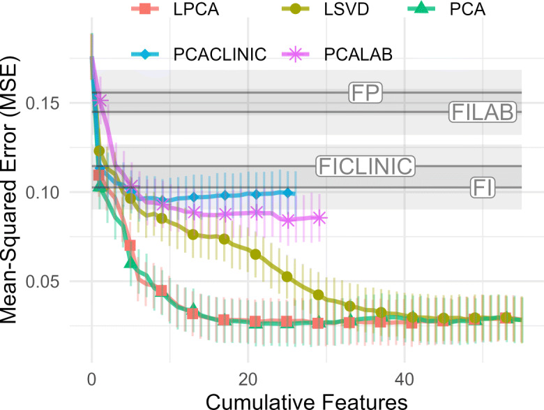
We decomposed and then reconstructed input variables using various dimensionality reduction techniques. In Fig. 3, we show the out-of-sample Youden index for the FI, PCA, LPCA, and LSVD, as indicated. For all, the first dimension dominates and represents $\sim 30\%$ of the gain in predictive power over guessing (a guess has Youden index = 0).

Fig. 3.

Cumulative compression. Tuning the size of the latent dimension bottleneck, we inferred the maximum number of dimensions required to efficiently represent the input data. The reader should look for two things: (1) the number of components (dimensions) needed to achieve a relatively high score, and (2) the slope of the curve — when it flattens we can expect the features are noise, variable-specific, or otherwise less important. Logistic SVD compresses the input most efficiently, saturating at around 30 features. Note the dramatic difference between lab and clinical compression both for PCA and the FI; the first PC of clinical data scores as well as 9 lab PCs. PCACLINIC and FICLINIC use only clinical variables; PCALAB and FILAB use only lab variables

LSVD was the most efficient compression technique, having perfect reconstruction after approximately 30 latent dimensions. However, this performance comes at a large cost in terms of number of parameters [33], and with respect to computational resources. Our benchmarks in Online Resource S3.6 indicate that PCA is about 10× faster than LPCA which is itself 10× faster than LSVD.

The information in the input variables includes both important, latent, information reflecting an individual’s health-state and variable-specific information which could be considered noise (i.e. not useful for predicting relevant outcomes). Generally, we see that the first dimension performs similarly for all methods. Additional dimensions are needed for accurate compression. The number of dimensions needed ranges from 30 (LSVD) to all 55 (PCA). This implies the dataset can be fully represented by a manifold of new features with dimensionality at most 30. We also see that clinical data compresses more efficiently than lab data, implying significant correlations between clinical variables. All four dimensionality reduction techniques estimated a very similar first dimension, as indicated by their strong mutual correlations, shown in Fig. 4. The correlation between the FI and PC1/LPC1/LSV1 is almost perfect, ρ > 0.95, with nearly identical age and sex dependencies (Fig. S19). Centering had a negligible affect on results, only reducing the correlation to ρ > 0.9. This implies that a very strong signal is present in the data and that it is very close to the FI, particularly the FI CLINIC.

Fig. 4.

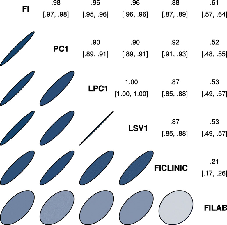
Spearman correlation of primary features across algorithms. The first latent dimension for either PCA, LPCA, or LSVD correlated strongly with the FI and each other, and correlated more strongly with the FI CLINIC than FI LAB. This implies a strong mutual signal very close to the FI, especially the FI CLINIC. Upper triangle is correlation coefficient with 95% confidence interval. Ellipses indicate equivalent Gaussian contours [51]

In Appendix A.2, we show how the equivalence between the FI and PC1 can arise from the structure of the joint histogram and provide conditions under which the FI/PC1 is the dominant dimension.

Feature associations

While compression efficiency identifies the number of dimensions needed to recover the input data, it does not tell us how the information is split across features, nor how that information relates to adverse outcomes.

We explore the flow of information by investigating the associations between each observed variable and each latent feature, e.g. the FI, each PC. We used the metrics described in the “Performance metrics” section, which range from 0 (no association) to 1 (perfect association). A score of 1 means that if we know the value of the feature then we can perfectly predict the value of the associated variable. We automatically picked the Youden index greater than 0, reflecting the arbitrary direction of the association.

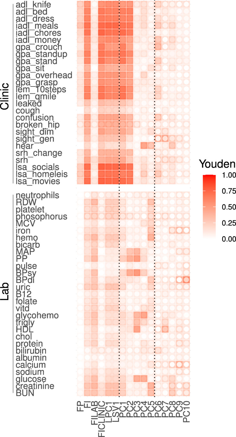
In Fig. 5, we present the Youden index for predicting the input variables, i.e. compression ability. We can infer the information content of each feature through the scores — a higher score implies more information related to a particular input variable. Similarly, in Fig. 6, we score the association strength of each feature with each outcome. In both figures, the inner colour indicates the lower limit of the 95% CI: lighter values are less significant (white is non-significant). Consistent with the compression observations, we see nearly identical patterns between the FI and the first latent dimension: PC1, LPC1, and LSV1; note also the similarity to the FI CLINIC. We have included PCs up to 10 as input variables. We observe higher PCA dimensions tend to be weaker, but also more specific predictors.

Fig. 5.

Feature associations with individual input variables, i.e. what goes into each feature. Youden index (fill colour) quantifies strength of associations between features (x-axis) and health deficits (y-axis); 0, no association; 1, perfect. Note the similarity of the FI, FI CLINIC, LPC1, LSV1, and PC1. Inner circle fill colour is the lower limit of 95% CI (white is non-significant). Higher PCs show no/low significance

Fig. 6.

Feature associations with individual outcomes, i.e. what we get out of each feature. Association strength (fill colour) between features (x-axis) and adverse outcomes (y-axis); 0, no association; 1, perfect. Note the similarity of the FI, FI CLINIC, LPC1, LSV1, and PC1. Inner circle fill colour is lower limit of 95% CI (white is non-significant). Higher PCs show no/low significance. Text on right denotes accuracy metric used

Generalized linear models (GLMs)

The feature associations give an idea of what information is in each latent variable but they do not consider the contributions that multiple latent variables can make towards prediction. Our GLMs do this, and so allows us to see how many latent dimensions are needed to predict outcomes well.

The cumulative predictive power conditional on all available information up to the N^th PC/LPC/LSV is given in Figs. 7 and 8. We have included demographic information as the 0^th feature, and are again estimating out-of-sample performance. We see that the discrete outcomes (Fig. 7) require few dimensions to achieve near-maximum performance. Conversely, continuous outcomes (Fig. 8) require many dimensions. Overfitting appeared to be present in the highest dimensions, as demonstrated by a drop in performance as the cumulative number of features becomes larger (Fig. 7). Overfitting was much worse in the complete case data, ostensibly due to outcome rarity (Fig. S41). When choosing the number of PCs to use, the optimal balance between overfitting discrete outcomes and under-fitting continuous outcomes seemed to be at approximately 20 latent dimensions for both PCA and LPCA. It is interesting that LSVD, which was best at compression, required more dimensions, approximately 40, to predict continuous outcomes well. This suggests that LSVD could be susceptible to overfitting when case data are scarce.

Fig. 7.

Cumulative prediction plot for discrete outcomes (GLM). 0th dimension is demographic information. Increasing the number of features initially improves prediction but eventually it gets worse due to overfitting. LSVD performs notably worse than PCA and LPCA. Youden index: higher is better

Fig. 8.

Cumulative prediction plot for continuous outcomes (GLM). 0th dimension is demographic information. Increasing the number of features improves prediction monotonically. LSVD performs notably worse than PCA and LPCA. MSE is on standarized scale; therefore, R² = 1 − MSE. MSE: lower is better

We observed strong similarities between PCA and LPCA both in compression (Fig. 3) and prediction (Figs. 7 and 8). In Appendix A.4, we demonstrate that, under reasonable asssumptions, PCA is the single-iteration approximation of LPCA, which explains the similarities.

For specific outcomes, the performance of the GLM using PCA is shown in Fig. 9, grouped by type. Consistent with Fig. 7, medical conditions, disability, and survival (all binary) tend to have low-dimensional representations and do not benefit from more than a few PCs: typically PC1 is sufficient. Note the difference between the FI CLINIC and FI LAB, with the former being perfectly reconstructed by 2 PCs, whereas the latter required many more.

Fig. 9.

Improvement in predictive power as more PCs are included, grouped by outcome type (GLM). Coloured lines indicate specific outcomes, and black line indicates the mean for each group. For most outcomes, the performance stops improving after a few PCs, hence why we have truncated at PC6. The exceptions are explored in Fig. 10. Note: legend is sorted from best (top) to worse (bottom) performance of the PC6 model. See Fig. S21 for the complete plots without truncation. Subplots represent outcomes grouped by type, as indicated (“a–f”)

In Fig. 10, we highlight selected outcomes which showed high-dimensional behaviour. These were variables that we visually observed in Fig. 9 to have positive slopes up to several PCs (excluding the FI LAB because it shares input variables with PCA). We include FP as a reference system that is theoretically high-dimensional [52]. Several of the high-dimensional outcomes are related to biological systems that integrate information from many subsystems: inflammation and metabolism, as well as age itself. Note that microalbuminuria is connected to many different systems as a biomarker of microvasculature damage [41].

Fig. 10.

Improvement in predictive power as more PCs are included, high-dimensional outcomes (GLM). Outcomes were hand-picked variables based on requiring many PCs to achieve maximum performance. The FP was included for comparison. We tend to see continual improvement for the discrete and continuous outcomes, excluding the FP (up to $\sim$10). Age appeared to be the highest dimensional. Subplots represent high-dimensional outcomes grouped as continuous, (a), or discrete, (b) along with age as the lone outcome, (c)

In Online Resource S3.3, we repeated the stepwise GLM using either LPCA or LSVD. We observed only minor differences between LPCA and PCA (Fig. S24). LSVD showed much larger differences than PCA, in particular it achieved lower overall accuracies (Fig. S25). In all cases, our qualitative results remain unchanged. We also considered non-linear behaviour by including quadratic and interaction terms between the PCs but found no improvement and a tendency to overfit (Fig. S22), suggesting that the linear model is optimal for the available data.

Robustness analysis

PCA defines a particular linear transformation (rotation) between the original variables and a new “latent” space. An important question is reproducibility of this latent space: can it be robustly estimated from the data?

We bootstrapped the sample to estimate the robustness of the linear transformation that rotates the data into PCs. The resulting rotation matrix up to the 10th PC is displayed in Fig. 11. The exact values are in Table S7. Note the overall sign of each PC is arbitrary [18]. We observed that the first 4 PCs were reliably estimated, 5 and 6 were marginally robust; the remaining PCs were too noisy to be consistently estimated. The loss of robustness could be due to PC features swapping order due to small changes in their associated eigenvalues (see Fig. 12), which could be addressed by a matching algorithm. On the other hand, the first 4–6 PCs appear to be robust and generalizable across the sample population.

Fig. 11.

PCA robustness. Robustness of the PCA rotation was assessed by randomly sampling which individuals to include (i.e. bootstrapping, N = 2000). Left side are lab variables; right are clinical. Inner circle fill colour is 95% CI limit closest to 0. Grayed out tiles were non-significant. The first three PCs were quantitatively robust. We see the robustness drops with increasing PC number. The global sign for each PC was mutually aligned across replicates using the Pearson correlation between individual feature scores. In Fig. S27, we assessed robustness by randomly sub-sampling input variables and again observed that PCs 1–3 were robust

Fig. 12.

PCA second moments (eigenvalues) with bootstrapped standard errors (N = 2000). Log-log scales. Note the bilinear structure. Banded region is optimal performance region (± 1 error bar from best using Figs. 7 and 8). In all three variable sets, eigenvalues curved away from second line just before overfitting started

PC1 is very close to the full FI (lab + clinical), as shown in the “Input compression” section, and we observe in Fig. 11 that PC1 has nearly uniform weights for each variable, explaining the underlying similarity. Both the FI and PC1 are (nearly) unweighted averages of deficit variables. PC2 suggests that the next most important term to the full FI is a contrast term splitting lab and clinical inputs into their respective domains. PC3 has a similar structure of contrasting domains of blood pressure and metabolism. In Online Resource S3.4, we confirmed the robustness of the first 3 PCs to choice of variables by randomly selecting variable subsets of size 30, the remaining PCs did not appear to be robust (Fig. S27).

The corresponding second moments — i.e. eigenvalues — of the PCs are given in Fig. 12. A bilinear structure was apparent in the log-log plot. In time series analysis, others have attributed this PC structure to fractal dimension [53], indicating a potential connection to complexity [54]. Values curved below the second line after approximately 20 PCs for the complete data, around 15 for the clinical data, and around 12 for the lab data. These values correspond to the end of the optimal-model regions in Figs. 7 and 8 (represented as bands in Fig. 12); the curved region may therefore provide a useful heuristic for identifying less relevant PCs that exacerbate overfitting.

Note that the PC rotation does not have to be robust for it to be useful, for example PCA can be trained on one sample and used on another. Differences between the samples would then change the eigenvalues (via Eq. A8) and PC ranks. Practically, this means performing feature selection after PCA, either by inspecting the eigenspectrum (e.g. Fig. 12) or by using an automated algorithm such as LASSO [49].

Age stratification

We investigated the effect of cohort age on our results. The joint 2D histogram tended to saturate (increase in magnitude) with age, although the qualitative structure of the histogram was stable (Online Resource S3.5). This implies that the PCA features — which are derived from decomposing the 2D histogram — do not change much with age. The increasing saturation does increase the relative contribution of the first PC with age, however. The first eigenvalue increased with increasing age quartile from 0.352(3) for ages 60–65 to 0.330(3) for ages 65–72 to 0.405(3) for ages 72–81 to 0.473(3) for ages 81+, as seen in Fig. S30.

To investigate a potential age effect further, we split the population at the median age (72) then redid the analysis using a young cohort (age < 72) and an old cohort (age 72+). (Note that we excluded demographical variables in this comparison because the baseline model, i.e. covariates as the only predictors, may not be equally powerful for both cohorts, confounding direct comparison.) Compression was similar for both cohorts (Fig. S31). Prediction using the GLM, however, was notably different (Fig. S32). For discrete outcomes, the cohorts scored similarly, the young cohort had a maximum Youden index of 0.333(15) compared to the older cohort which scored 0.326(13). For continuous outcomes, the young cohort performed much worse with a minimum MSE of 0.134(20) compared to the older cohort with 0.055(19).

We summarize the variable-specific compression and prediction using GLMs in Online Resource S3.5. The results were qualitatively similar, indicating robustness with respect to age. The GLM Youden indexes for compressing each predictor showed a stronger focus on predicting creatinine and BUN in the older cohort than in the younger cohort. The younger cohort tended to prioritize other predictor variables, e.g. glucose, HDL, and iron (Fig. S33). The GLM scores for predicting outcomes also showed microalbuminuria, and to a lesser extend gait, were better predicted in the older cohort (Fig. S34). Most of the differences we observed between the young and old cohorts were strongest in the higher PCs, and this reflects the lack of robustness of the higher PCs that we observed in Fig. 11.

Discussion

The first latent dimension “is” the frailty index

We performed dimensionality reduction on binarized health data encoded as normal (0) or dysfunctional (1). The first dimension of each algorithm, PCA, LPCA, and LSVD, indicated a strong signal with general predictive power both for deficit compression and adverse outcome prediction. This first latent dimension correlated almost perfectly with the FI (Spearman ρ > 0.95), reproduced the same gender and age trajectories as the FI (Fig. S19), and had very similar associations (Figs. 5 and 6).

What underlying phenomenon is this first latent dimension capturing? The FI is a measure of frailty [21], making it the primary suspect. Indeed, frailty is strongly associated with adverse outcomes [5] and the first latent dimension strongly predicted almost all outcomes. Specifically, the first latent variable predicted the five key frailty outcomes: exhaustion, weakness, physical inactivity, gait, and weight (BMI). Frailty has been strongly associated with inflammation, total and HDL cholesterol, hyperglycemia, and insulin resistance [55]. Consistent with this, we observed a (weak) relation between the first latent variable and HDL/total cholesterol, a (weak) relationship with the inflammation biomarker CRP, and a (moderate) relationship with glucose and glycohemoglobin. We saw stronger relationships with clinical measures: IADL/ADL disability, exhaustion, and gait, all three of which are important signs/symptoms of frailty [55]. IADL/ADL disability is known to be strongly related to frailty and specifically the FI [56].

What is behind the approximate equality of FI and PC1? We see in Fig. 2 that the 2D histogram for PC1 is approximately a large block of uniformly correlated variables. In Appendix A.2, we show how an exact block structure leads to PC1 ≈FI and that the FI becomes an increasingly good approximation for the information in the entire 2D histogram as the number of variables increase — saturating past approximately 30 variables. Indeed, others have reported moderate-to-strong correlations between all variables and equal associations/weightings to the first PC [27].

We hypothesize that the selection criteria for the FI [6] ensure that the joint histogram has this universal correlation structure between many variables: all deficit variables must (1) be related to health status, (2) increase in prevalence with age, (3) cannot saturate in youth, and (4) should contain “at least 30-40” variables [6]. These conditions are likely to lead to moderate-to-strong correlation between deficits due to their mutual age dependence through an individual’s biological age (overall health state) [57]. These correlations then lead to $\text{PC1}\simeq \text{FI}$.

To summarize, the FI is an excellent summary measure for a large collection of moderate-to-highly correlated health deficit variables. That is, the FI acts as a “state variable” which summarizes the health state of an individual [20]. Under such conditions, the FI approximately equals PC1 and can describe the collection of health deficit variables with little residual information, as has been empirically observed [30]. In turn, PC1 approximates the more appropriate loss function provided by LPCA (Appendix A.4). The ease with which the FI, PCA, and other methods detect a very similar primary signal suggests that any good dimensionality reduction algorithm would identify it as the dominant signal in health deficit data. This signal predicts important outcomes and can be easily estimated via the FI or PC1.

PCs represent scales of dysfunction

PCs should be interpreted as building blocks consisting of coarse grained scales that can be added together to efficiently represent common patterns of dysfunction — adverse outcomes and health deficits. While others have discussed the biological significance of individual PCs, for example as dietary patterns [28] or up/down inflammation regulators [26], it is unlikely that the PCs in the present study represent specific diseases or adverse conditions (excluding PC1). This is because the PCs must be statistically independent, while the first PC already represents generic dysfunction akin to the FI [4, 5]. Hence, any biological pattern of dysfunction using PCA should include a non-trivial contribution from PC1. Therefore, PCs past PC1 are unlikely to represent specific pathways of dysfunction.

Instead, we should look for the minimum number of PCs to combine to construct a known pattern of dysfunction. For example, we can cross-reference Fig. 11 against upticks in Figs. 9 or 10. Low PC1 plus low PC2 gives global clinical dysfunction with agnostic lab, which is tantamount to the FI CLINIC. This explains why PC1 plus PC2 reconstructed the FI CLINIC. Low PC1 plus high PC2 gives quasi-global lab dysfunction with agnostic clinic, with strong cardiovascular dysfunction, such as would be seen in metabolic syndrome [58]. Adding low PC3 would give metabolic dysfunction alone, and this explains why inclusion of PCs 1–3 gives a sudden improvement in BMI, obesity, and diabetes prediction. If we then add high PC4, we could get dysfunctional glucose metabolism alone, which explains the uptick in diabetes prediction with inclusion of PC4 [41, 59]. PCA provides an efficient coarse graining procedure such that many common patterns of dysfunction are efficiently represented as sums of PCs.

How does PCA achieve this? PCA identifies domains of variables likely to be mutually deficient, i.e. strongly correlated. In this manner, PCA coarse grains by concatenating domains in a PC (e.g. PC 1 contained all domains), approximating them as a block, and then in the next PC it can contrast those domains with opposing signs to account for the stronger within-domain correlations than between-domains (e.g. PC 2 splitting lab and clinical). In this way, the PCs encode domain-specific information, similar to the way experts have manually created domain-specific FIs [23]. Understanding health using multiple domain-specific FIs may be helpful for interpretability but could also make the analysis vulnerable to issues related to collinearity, such as unreliable regression coefficients [18]. In contrast, PCA is high-throughput, and PCs are uncorrelated, making PCA a better foundation for quantitative approaches — including pre-processing [24] before mapping into domains.

An alternative route to improving interpretability is through formal latent variable modelling. For example, grade of membership simultaneously infers health “profiles,” along with individual scores for each profile, which are similar to PC scores [35–37]. The primary advantage that we see in PCA is that it compresses information into the lowest PCs by systematically estimating the direction of highest variance, followed by second highest, etc. This yields a set of optimal representations [18], and makes it particularly easy to quantify the information lost by picking a smaller representation. For example, Fig. 3 shows the efficiency of each representation from 1 dimension up to the number of input dimensions. PCA also has several practical advantages over formal latent variable models: it is simple, fast, convex, easily tuned, reversible, and standard in statistical software packages, such as R [48]. Because of this, PCA can be easily integrated into an existing analysis pipeline as a pre-processing step.

PCA appears to generalize the action of the FI. The FI treats all health deficits as indistinguishable, such that you can pick any 30+ and expect to get the same summary health measure (subject to selection criteria) [6]. $\text{PC1}\simeq \text{FI}$ adopts indistinguishability of deficits from the FI. PC2 is able to “see” (discriminate) the difference between lab and clinical deficits, but cannot distinguish individual lab variables from lab nor clinical from clinical. For example, we expect PC1 and PC2 will change little if a new admixture of lab and clinical variables are used — while higher PCs will change more. PC3 is able to “see” the difference between metabolic, heart-related vs other deficits, and so forth for higher PCs. Within each PC, the exact variables used should be unimportant, as long as they come from the same domains.

Domains in lab vs clinical data

We see that dimensionality reduction algorithms treat clinical and lab data domains differently, and are sensitive to domain boundaries. Strongly mutually dependent variables form block-like domains in the joint histogram, which can be efficiently represented by a single latent dimension, making them preferred targets of PCA (and LPCA).

Clinical variables were strongly associated with a single latent variable whereas lab variables spanned more dimensions. For example, comparing the FI CLINIC to FI LAB in Fig. 9: the FI CLINIC was almost completely described by 1 PC whereas the FI LAB required at least 5. Inspecting the 2D histogram (Fig. 2), we can see that the clinical data have stronger inter-dependencies than the lab. Previous research has shown that clinical variables are sufficiently compressed by a single dimension [30], whereas lab variables need at least two [31]. We did see an indication of high-dimensional clinical data in the pooled continuous outcome prediction of clinical PCA, which improved up to 5–6 PCs, probably due to improvements in CRP, BMI, gait, and/or age (which were high-dimensional).

Clinical deficits tend to accumulate over time and are efficiently described by the FI CLINIC. In contrast, the lab data are more complex, reflecting the diversity of biological systems the lab data represent, for example: metabolic (e.g. cholesterol and glucose [60]), immune (e.g. neutrophils [61] and CRP), renal (e.g. creatinine and BUN [62]), and cardiovascular (e.g. blood pressure [62]). Ostensibly, there are too many directions for dysfunction to proceed in to be completely captured by a single summary measure such as the FI LAB alone. For example, an individual may be prone to metabolic dysfunction, as indicated by dysfunctional glucose and glycohemoglobin, whereas another may have a weak heart, as indicated by dysfunction blood pressure, or weak kidneys. Why should these individuals accumulate (and propagate) dysfunction, or damage, in the same way? Our results indicated that they do not; multiple dimensions of PCs are needed to represent the diverse phenotypes of dysfunction captured by lab data. In contrast, the clinical data appears considerably more homogeneous.

Clinical data therefore seem to contain more generic (albeit crucial) information than lab data, with only a few dominant PCs in the former but more PCs needed in the latter. This may reflect the improved resolution of biological dysfunction in lab data. For example, lab data can resolve heart disease from hypertension vs from chemotherapy toxicity, but the clinical consequences of heart disease are the same either way. Inclusion of molecular data, such as metabolomics, proteomics, or genomics, in future studies would clarify whether this trend towards more PCs continues as biological resolution is further increased.

The underlying univariate structure of the clinical data means that when we calculate the FI with equal weightings we are favouring the strongly correlated clinical deficit data over the weakly correlated lab data. PCA targets large, dense blocks of highly correlated variables. In the present study, the clinical data formed a dense block of the same size as the lab data and were therefore preferred targets. Conversely, we expect that a very large block of weakly correlated variables would be a preferable target over the relatively small number of clinical variables. Thus, if we had included an exceptionally large domain, e.g. “omics” data with thousands of features, then it could dominate any much smaller domain. How would we know if there is a problem? We can look for blocks in the 2D joint histogram: a large block indicates strong mutual dependence, which will drag most algorithms towards it. A two-stage, hierarchical dimensionality reduction procedure, homologous to the “bifactor” model of [31], would mediate such an effect, and would be a good starting point for “omics” data. One could do PCA on each domain, take the most important PCs from each domain, and then perform PCA on all of the top PCs.

The dimensionality of integrative systems

“High-dimensional” outcomes required many PCs to fully predict. If an outcome relies on integrating information from many domains then we should see an incremental improvement as we move from PC1 to higher PCs. For example, prediction of age continually improved until about PC20. This is indicative of a high-dimensional, integrative process that accumulates dysfunction over several domains/scales and we therefore surmise, many different pathways of dysfunction. Stated equivalently, these are systems that function in many different ways.

CRP and chronological age showed the highest dimensionality, ostensibly integrating information from many domains. CRP is an inflammation biomarker indicative of altered cellular communication, the latter has been called an “integrative hallmark of aging,” meaning that it indicates a phenotypic accumulation of damage [1]. These outcomes may be indicators of accumulated damage across domains and, ostensibly, scales. The approximately 20 PCs needed by age represents information integrated over all domains, probably leaving only noise in the remaining PCs (Fig. 12). In regressing against age, we are generating a biological age model [57]. Such a model is effectively condensing 20 dimensions of age-related decline into a single measure. This explains why there exists many partially overlapping biological ages [12, 13]: each biological age represents a different one-dimensional projection from a high-dimensional latent space. All of these ages contain overlapping contributions from the first latent dimension due to its strong explanatory power.

In contrast, medical conditions, ADL/IADL disability, survival, and FP all seem to have one dominant dimension: PC1. For these outcomes, the first PC predicted almost as well as including all 55. This means that the only dimension we know is useful for predicting these outcomes is the dimension representing generic health deficits. This implies that our knowledge of these outcomes lies on a line: things go wrong in just one direction.

Money difficulty and difficulty preparing meals, both IADL, were notable exceptions that depended on higher PCs, notably PCs 6–8. These were the most cognitive-intensive clinical outcomes, which suggests that cognitive decline has its own domains of dysfunction captured by later PCs, and is consistent with what others have observed via factor analysis [63]. This highlights the critical difference between outcomes which appear to integrate information across multiple scales/domains, such as chronological age, versus those that depend on specific domains beyond a low rank PC representation, such as difficulty preparing meals. The former should show continual improvement as the number of PCs increases whereas the latter should show sudden improvement when a specific PC is included (e.g. compare the curves for predicting age versus difficulty preparing meals, iadl_mealDIS in Fig. 10, the former improves with each additional PC).

Practical considerations

The FI’s ability to effectively compress the salient information within a set of binary health deficits appears to be due to a dominant underlying signal that is readily identified by various dimensionality reduction techniques. PCA is the most common, robust, simplest, and fastest. LPCA is a more complex algorithm that can enhance compression without loss of predictive power. LSVD is too focused on compression to yield good predictive features; it is also much slower. However, any of these techniques can be used to extend the dimensionality of the FI.

A critical aspect of our central hypothesis — that efficient representations of health deficits are efficient representations of adverse outcomes — is that biomarkers must be converted to a standardized dysfunction scale. Sample-specific scales, such as the standard deviation, run the risk of propagating sample population idiosyncrasies or healthy variation. In contrast, deficit thresholds have been expertly tuned. Applying PCA directly to continuous biomarker data without converting to a standardized dysfunction scale may result in features that primarily capture healthy variation and/or have no clear connection to adverse outcomes.

We have focused on dimensionality reduction using compression algorithms, which do not depend on any specific outcomes. Dimensionality reduction could also be used with specific outcomes [19], or could simply be used with some of the adverse outcomes as input variables — for example medical conditions like diabetes and heart disease [40].

As we observed with LSVD, while compression seeks an efficient representation of the input it may not also be efficient for prediction. We hypothesized that efficient representations of health deficits would also be efficient representations of adverse outcomes. It is thus a surprise that we observed LSVD compressing so well, given its relatively poor predictive performance. Since LSVD has many more parameters than either PCA or LPCA, this could be a manifestation of overfitting to the input data, i.e. finding population-specific features rather than health-specific features.

Both PCA and LPCA are designed to handle cross-sectional data, although we expect they will also be useful for longitudinal data. Both are based on reversible linear transformations which preserve information, and hence they can be applied to new populations or measurement waves without loss of information. If the PCs/LPCs are expected to remain constant over time then we can simply pick a convenient wave to compute the transformation, probably the first, then apply the transformation to all other waves. This would be a viable approach in the present study population, since we observed that the PC transformation did not depend on age (Online Resource S3.5). If the transformation changes between waves, then we would suggest to first combine the waves to learn a shared transformation, then apply it separately to each wave.

What additional utility does PCA provide over the FI? Each of the multivariate dimensionality reduction algorithms was at least as good at predicting any given outcome as the FI was. It is also clear from stepwise regression that truncated PCA can help to avoid overfitting; we can surmise that it would be particularly useful for avoiding the “curse of dimensionality” (when the number of predictors meets or exceeds the number of individuals). The only downside to a multivariate approach is the increased computational complexity, which is minor for PCA.

How do we know the right number of features (PCs) to use? Conventionally, one looks for an “elbow” in the eigenspectrum, indicating a sudden drop in PC information content, or one picks the optimal number that maximizes prediction accuracy for a desired outcome [18]. PCs with small eigenvalues are, by our choice of normal/dysfunctional scale, minor corrections to the 2D deficit histogram which we hypothesize are unimportant for predicting adverse outcomes. In the present study, we observed that the eigenspectrum had a distinct bilinear structure in the log-log plot, and inferred that when eigenvalues drop below the second line, it is an indication of a drop in PC importance. Others have noted small eigenvalue PCs were significant predictors of mortality [24]; we hypothesize that these PC eigenvalues would lay on the second line (but not below). Our proposed method of finding the “elbow” can be used to automatically identify the number of PCs to use without needing to refer to any particular outcome. Other fields have shown that there is an unmet need for unbiased PC selection criteria such as ours [29].

We observed little change in PCA performance with age. One minor change was in the relative importance of certain biomarkers/outcomes, as indicated by the PC order in which they appeared. The primary age effect was a monotonic increase in overall deficit frequency with age, a phenomenon that is well known from the FI [64]. Although the 2D histogram thus became increasingly saturated with age, normalizing by the mean FI showed that the histogram structure was not changing, only the global deficit frequency. This suggests that the canonical pathways of dysfunction do not change with age, rather they saturate.

We note a few sources of error. Data imbalances can negatively affect performance measures and model fits; hence, we focused on the Youden index and used a weighting scheme for the GLM. Most of the clinical variables used as inputs were related to physical activity which may skew our interpretation, although other researchers have used a similar set [40]. Our clinical variables were self-reported rather than observer assessed, which may affect performance [65] although it is unclear how [23]. The main weakness of this study is our use of a single population. We used cross-validation and performed a robustness analysis to estimate precisely the effects for the sample population, but there may be study or population–specific effects in our results. However, the complete case data provided a subpopulation of younger, healthier individuals, and yielded similar conclusions (Online Resource S4).

We have also neglected to include social vulnerability deficits, which contain additional predictive power over the FI alone [66], although we did include partner status, education, and income as covariates. It is curious to consider how PCA would handle grouping domains of information such as social vulnerability and observer vs self-reported health deficits — we expect it would modify the PCs to find these new domain boundaries.

Future directions

Our work has been motivated by the need for estimating summary measures of health from new domains and with multiple dimensions. PCA may provide a useful extension of the FI to higher dimensions. Other approaches are also worth exploring, such as non-negative matrix decomposition [67], variational autoencoders [68], or kernel PCA [69]. Nested approaches may be useful for dealing with domains with many variables e.g. “omics” data. Our ability to robustly estimate latent dimensions also provides an opportunity for more interpretable latent variable modelling, for example structural equation modelling or factor analysis [31]. The stability of the PC rotation with age may also make it a useful pre-processing step for longitudinal analysis, such as for dynamical modelling. PCs can reduce dimensionality and likely have simplified interactions.

PCA appears to have additional utility. If the “elbow” we observed in the PC spectrum is caused by a transition from signal to noise, it may be useful for denoising, which has been identified as an important issue with epigenetic clocks [24].

Conclusion

We compared several dimensionality reduction algorithms for their ability to compress health deficit data and predict adverse outcomes. The FI, PCA, LPCA, and LSVD all identified the same dominant signal. This demonstrates and explains the FI’s uncanny ability to predict adverse outcomes. We found that the additional dimensions estimated by PCA were helpful for better capturing health outcomes, particularly integrative systems such as inflammation, metabolism, and chronological age. Such systems were sensitive to many dysfunction pathways, domains, or scales. PCA is a simple tool that can help researchers to identify and efficiently represent multidimensional biological systems in aging research.

Electronic supplementary material

Below is the link to the electronic supplementary material.

Appendix: . Binary PCA

We seek an efficient representation for binary health data: normal (0) or deficit (1). Equivalently, we are seeking (1) a basis set, (2) a set of features, or (3) a set of composite health measures. Representation efficiency is commonly measured by compression. Compression is the ability to take a set of p input variables, reduce (“compress”) them into k < p latent variables, and be able to reconstruct the original p input variables from these k latent variables. Compression fidelity is measured by a loss function that compares the original input variables to the reconstructed inputs.

Each dimensionality reduction technique is the optimal solution to a particular choice of loss function. If we require independent (orthogonal) features and minimize the mean-squared error then the solution is given by PCA (see below). The mean-squared error is not ideal for binary data, however, since we only need to know whether a variable is larger or smaller than 0.5. More appropriate choices for binary data lead to LPCA [33] and LSVD [33, 34]. The performance gains of these methods over linear PCA have been modest [33, 34], and may not justify the increased algorithmic complexity. When we refer to PCA, we mean conventional, linear PCA.

In finding the directions of maximum variance, PCA decomposes the covariance matrix into its eigenvectors. For binary healthy/deficit data, the covariance matrix takes on a special meaning. The (uncentered) covariance matrix is equivalent to the 2D pairwise joint deficit frequencies, with the diagonal corresponding to the individual variable’s marginal probability (i.e. deficit frequency). Binary PCA effectively compresses all of the marginal and pairwise deficit probabilities into a set of features of decreasing importance. We refer to each feature as a latent dimension.

A.1 Problem formalization

We seek an orthogonal basis set of features to efficiently represent the data. Orthogonality ensures that features are independent (uncorrelated) and that each individual has a unique representation in terms of the basis [70].

Let ${\overrightarrow{\varphi }}_i$ be the i th basis feature, we want to minimize the reconstruction error between the N × p data matrix, X, in its original state and after bottlenecking through the (latent) feature space of size k ≤ p. The representation of the i th individual and j th deficit from our data in the new space is given by:

$${\widehat{X}}_{ij}\equiv \sum _{n=1}^k{Z}_{in}{\varphi }_{nj},$$ A1

where Z_in represents an individual’s feature score and ${\widehat{X}}_{ij}$ is our best estimate of the reconstructed input data, X_ij.

Using the orthogonality of the ${\overrightarrow{\varphi }}_i$, we estimate the feature scores using the inner product,

$$Z_{in}=\sum _{j=1}^p{\varphi }_{nj}{X}_{ij}$$ A2

thus,

$$\begin{array}{rcl}{\widehat{X}}_{ij}& =& \sum _{j=1}^p\sum _{n=1}^k{\varphi }_{nj}{X}_{ij}{\varphi }_{nj}\\ & =& \sum _{j=1}^p{X}_{ij}\sum _{n=1}^k{\varphi }_{nj}{\varphi }_{nj}\\ & =& \sum _{j=1}^p{X}_{ij}\sum _{n=1}^k{U}_{jn}{U}_{nj}^t\\ \Rightarrow \widehat{X}& =& XU{U}^t\end{array}$$ A3

where U is the p × k matrix formed by having i th column equal to the i th basis, ${\overrightarrow{\varphi }}_i$, and U^t is the transpose of U.

For simplicity, convexity, and robustness, we assume the mean-squared error function; hence, we have:

$$\underset{\{{\overrightarrow{\varphi }}_i\}}{\min }\sum _{i=1}^N\sum _{j=1}^p\left(\right)X_{ij}-{[U{U}^t{\overrightarrow{X}}_{i\cdot }]}_j{\left)\right)}^2\text{with}\sum _{j=1}^p{U}_{ji}{U}_{jk}={\delta }_{ik}\mathrm{.}$$ A4

This is the Pearson formalism of PCA (where the mean has not been subtracted) [33]. Z ≡ XU^t is the PC score matrix and U is the rotation matrix. This formalism can be solved sequentially for each ${\overrightarrow{\varphi }}_i$ and is equivalent to picking the rotation of the data such that the first direction, Z_i1, has the maximum second moment (eigenvalue), the second direction has the second largest, and so forth [18].

The solution to Eq. A4 is found by eigen-decomposition of X^tX [18]. Each of the columns of U, ${\overrightarrow{\varphi }}_i$ satisfies

$$\frac{1}{N}{X}^{t}X{\overrightarrow{\varphi }}_i={\lambda }_i{\overrightarrow{\varphi }}_i\text{where}{\overrightarrow{\varphi }}_i\equiv U_{\cdot i}$$ A5

where λ_i is the i th eigenvalue and X^tX/N is the 2D histogram of joint frequencies of the binary input variables, with the diagonal equal to the 1D frequencies. This implies (using $X^{t}X\approx X^t\widehat{X}$, Eqs. A3 and A5),

$$\frac{1}{N}{X}^{t}X\approx \sum _{i=1}^k{\lambda }_i\left(\right){\overrightarrow{\varphi }}_i\otimes {\overrightarrow{\varphi }}_i\left)\right)$$ A6

with equality when k = p. ⊗ denotes the outer/tensor product and the terms are sorted by decreasing strength. Intuitively, we are forming the 2D histogram, X^tX/N, then decomposing it into a set of rank 1 matrices — i.e. square blocks — sorted by relative contribution; Fig. 2 illustrates the process for our dataset.

The principal components (PCs), P ≡ Z, are defined as the initial data transformed (“rotated”) into the latent space,

$$P_{ij}\equiv \sum _{k=1}^p{X}_{ik}{U}_{kj}$$ A7

using the eigen-decomposition, Eq. A5, we can show that the norm of each PC is determined by its eigenvalue (substituting U for ϕ),

$$\begin{array}{rcl}& & \frac{1}{N}\sum _k\sum _j{X}_{nk}^t{X}_{kj}{U}_{ji}={\lambda }_i{U}_{ni}\\ & \Rightarrow & \frac{1}{N}\sum _n\sum _k\sum _j{X}_{nk}^t{X}_{kj}{U}_{ji}{U}_{nm}={\lambda }_i\sum _n{U}_{ni}{U}_{nm}\\ & \Rightarrow & \frac{1}{N}\sum _k{P}_{km}{P}_{ki}={\lambda }_i{\delta }_{im}\end{array}$$ A8

hence the second moment of each PC determines its eigenvalue, λ, and therefore its order and relative importance. The sum of the second moments is conserved because U is an isometry [70].

A.2 Block histogram

There is a special 2D joint histogram pattern for which the first PC is equal to the FI for both logistic [33] and linear PCA (scaled by an irrelevant constant). When a uniform diagonal is on top of a dense, uniform, off-diagonal, the FI is the dominant eigenvector and is therefore the first PC.

More precisely, suppose the 2D joint frequency histogram, X^tX/N, is given by:

$$\frac{1}{N}{X}^{t}X=\left[\begin{array}{cccc}a& b& \dots & b\\ b& a& & ⋮\\ ⋮& & \ddots & b\\ b& \dots & b& a\end{array}\right]$$ A9

that is, the diagonal is constant, a, and the off-diagonals are also constant, b. This is a circulant matrix [71]. Note that a ≥ 0, b ≥ 0, and a ≥ b, because they are deficit frequencies ((X^tX)_ij = N〈x_ix_j〉 for binary variables x_i and x_j, clearly $\langle x_i^2\rangle \ge \langle x_i{x}_j\rangle$ so a ≥ b because $a=\langle x_i^2\rangle$ and b = 〈x_ix_j〉, where 〈x_i〉 is the mean of x_i). The eigenvalues of this circulant matrix are [71]:

$${\lambda }_k=a-b+b\sum _{j=0}^{p-1}{\left(\exp \left(\frac{2\pi }{p}ki\right)\right)}^j$$ A10

where k ∈ [1,p] is an integer and p is the number of columns in X (i.e. the number of variables); $i\equiv \sqrt{-1}$. If k≠p, the sum is a geometric series which converges to [72],

$$\begin{array}{rcl}{\lambda }_k& =& (a-b)+b\left(\frac{1-\exp \left(\frac{2\pi }{p}pki\right)}{1-\exp \left(\frac{2\pi }{p}ki\right)}\right)\\ {\lambda }_k& =& a-b\mathrm{k}\ne \mathrm{p}\end{array}$$ A11

If k = p, we instead have,

$$\begin{array}{rcl}{\lambda }_p& =& a-b+b\sum _{j=0}^{p-1}{\left(\exp (2\pi i)\right)}^j\\ {\lambda }_p& =& a+(p-1)b\end{array}$$ A12

because a,b ≥ 0 and a ≥ b we have that λ_p must be the first (largest) eigenvalue (assuming b > 0, otherwise it will be a tie).

The associated eigenvectors are given by [71],

$$U_{kl}=\frac{1}{\sqrt{p}}{e}^{-\frac{2\pi }{p}ikl}$$ A13

where k and l are integers. From Eq. A12, we know the first eigenvector is,

$$U_{pl}=\frac{1}{\sqrt{p}}\mathrm{.}$$ A14

Using Eq. A7, we can calculate the first principal component,

$$\begin{array}{rcl}{P}_{\cdot 1}& =& \sum _j\frac{1}{\sqrt{p}}{X}_{ij}\\ & =& \sqrt{p}\frac{1}{p}\sum _j{X}_{ij}\\ & =& \sqrt{p}\cdot \text{frailty index},\end{array}$$ A15

which is a constant times the FI. Hence if the joint histogram has the form of Eq. A9, the FI will coincide with the first PC. In the next section, we show the conditions under which the first PC is sufficient.

A.3 How well can we approximate the histogram?

The 2D histogram contains all pairwise frequencies (off-diagonals) and individual frequencies, making it an important summary of the information we know about the deficit statistics. How well does the first eigenvalue/eigenvector pair approximate the complete 2D histogram, given it has the special structure of Eq. A9?

From Eq. A6, we know that the eigenvalues/eigenvectors approximate the 2D histogram as:

$$\frac{1}{N}{X}^{t}X\approx \sum _{i=1}^k{\lambda }_i\left(\right){\overrightarrow{\varphi }}_i\otimes {\overrightarrow{\varphi }}_i\left)\right)$$ A16

with equality when k is equal to the number of variables, p (equal to the number of columns of X). Since the model is linear, we can summarize the mean-squared error using the coefficient of determination, R², and expect R² = 0 for a useless reconstruction and R² = 1 for a perfect reconstruction. Specifically,

$$R^2=1-\frac{{\sum }_i{\sum }_j{\left({(X^{t}X)}_{ij}/N-{\sum }_{l=1}^k{\lambda }_l\left(\right){\overrightarrow{\varphi }}_l\otimes {\overrightarrow{\varphi }}_l{\left)\right)}_{ij}\right)}^2}{{\sum }_i{\sum }_j\left(\right){(X^{t}X)}_{ij}/N{\left)\right)}^2}\mathrm{.}$$ A17

Using this, we compute the accuracy of the first eigenvalue/eigenvector pair in approximating the full 2D histogram,

$$\begin{array}{rcl}{R}^2& =& 1-\frac{{\sum }_i{\sum }_j\left(\right){(X^{t}X)}_{ij}/N-{\sum }_{l=1}^1{\lambda }_l\left(\right){\overrightarrow{\varphi }}_l\otimes {\overrightarrow{\varphi }}_l{\left)\right)}_{ij}{\left)\right)}^2}{{\sum }_i{\sum }_j\left(\right){(X^{t}X)}_{ij}/N{\left)\right)}^2}\\ & =& 1-\frac{{\sum }_i{\sum }_j\left(\right){(X^{t}X)}_{ij}/N-(a+(p-1)b)(1/p){\left)\right)}^2}{{\sum }_i{\sum }_j\left(\right){(X^{t}X)}_{ij}/N{\left)\right)}^2},\end{array}$$ A18

and substitute in the special form for X^tX/N,

$$\begin{array}{rcl}{R}^2& =& 1-\frac{{\sum }_i{\sum }_{j\ne i}\left(\right)b-(a+(p-1)b)(1/p){\left)\right)}^2}{{\sum }_i{a}^2+{\sum }_i{\sum }_{j\ne i}{b}^2}\\ & & +\frac{{\sum }_i\left(\right)a-(a+(p-1)b)(1/p){\left)\right)}^2}{{\sum }_i{a}^2+{\sum }_i{\sum }_{j\ne i}{b}^2}\\ & =& 1-\frac{p-1}{p}{(1-b/a)}^2\frac{1}{p(b^2/a^2)+(1-b^2/a^2)}\\ & & \end{array}$$ A19

where in the last line we emphasize there are only two tunable parameters: b/a is a measure of correlation strength and p is the number of variables. Both 0 ≤ a ≤ 1 and 0 ≤ b ≤ a are constrained because X is composed of binary variables.

There are two limits of interest. First, for b > 0 if we take b → a,

$$\begin{array}{rcl}\underset{b\to a}{\lim }{R}^2& =& 1-\frac{p-1}{p^2}\frac{{(a-b)}^2}{b^2}\\ & =& 1\end{array}$$ A20

this corresponds to a 2D histogram of perfectly dependent variables (which would be a rank 1 matrix). The other limit is taking a large number of variables with b > 0,

$$\begin{array}{rcl}\underset{p\to \infty }{\lim }{R}^2& =& 1-\frac{1}{p}\frac{{(a-b)}^2}{b^2}\\ & =& 1\end{array}$$ A21

which corresponds to an infinitely large 2D histogram. In both cases, R² = 1 and the first eigenvector — equal to the FI — is sufficient to perfectly estimate the 2D histogram and hence sufficient to completely describe the first- and second-order statistics. It is interesting to note the compatibility of the two limits which imply that getting a large, but finite, p and having b close to, but not equal to, a is likely to give R² ≈ 1.

In Fig. 13, we plot Eq. A19 for several values of the two free parameters, b/a and p. Nearly perfect R² is achieved for fairly modest values of b/a when p is sufficiently large. Interestingly, there is an apparent diminishing return for increasing p with an elbow at p ≈ 25, this is comparable to the 30 + deficits rule for the FI [6]. The 2D joint histogram in this study had a median diagonal value of a = 0.20 and median off-diagonal value of b = 0.04, giving b/a = 0.22 (p = 55; Fig. 2). We would then expect an ideal case to have R² = 0.84, the fit for our data yielded R² = 0.50 — large, but smaller than the ideal case.

Fig. 13.

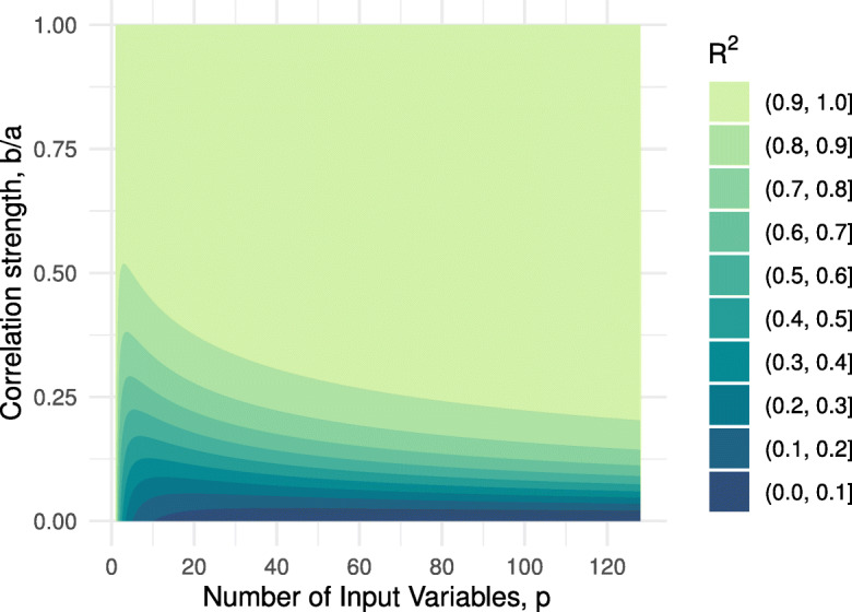
Special joint histogram approximation (Eq. A19). Fill is the R² fit quality for PC1 approximating the full histogram, given the histogram has the special structure given in Eq. A9. p is the number of features. a is the deficit frequency. b is the joint deficit frequency

This idealized, “toy,” model explains the approximate equivalence of the FI and PC1. What’s more, it allows us to estimate how dominant the FI/PC1 is. In the limit of a large number of variables and/or b ≈ a, we find that the FI/PC1 becomes a better approximation for the information in the 2D histogram. This is consistent with the observation that the FI is best used to describe a large number of correlated variables.

A.4 PCA approximates logistic PCA

Logistic PCA [33] minimizes the Bernoulli deviance, in analogy to the Gaussian formulation of linear (normal) PCA. The optimization problem is not convex but Landgraf and Lee [33] derive an iterative majorization-minimization scheme for solving the problem. We follow their approach and show that the first iteration of their loss function reduces to the same loss function as linear PCA. As a result, the estimated transformation, U, will be the same for either PCA or logistic PCA after the first iteration.

There are four steps to our adaptation of their approach:

1. Initialize U⁽⁰⁾ to be an orthogonal matrix. Pick k = p. Then, U⁽⁰⁾(U⁽⁰⁾)^t = I.

2. Initialize the mean, μ = logit(𝜖) where 𝜖 → 0⁺ is a small, positive number. This is akin to not subtracting the mean when we perform PCA.

3. Fix m ≡−μ. This is the main assumption. m should be a large, positive number [33]. Our definition of μ ensures that m is a large positive number.

4. Iterate the majorization-minimization algorithm [33] exactly once.

The initial ${𝜃}_{ij}^{(1)}={\widetilde{𝜃}}_{ij}$, due to the orthogonality of the initial U⁽⁰⁾. Note that ${\widetilde{𝜃}}_{ij}\equiv m(2X_{ij}-1)$ [33]. The loss function, Eq. (9) of [33], is then

$$\begin{array}{rcl}& & \underset{U}{\min }\sum _i\sum _j\left({\left[U{U}^t\left({\widetilde{𝜃}}_{i\cdot }-\overrightarrow{\mu }\right)\right]}_j-\left({\widetilde{𝜃}}_{ij}-\mu \right)\right)\\ & & {\left(-4\left(X_{ij}-\sigma \left({\widetilde{𝜃}}_{ij}\right)\right)\right)}^2\\ & =& \underset{U}{\min }\sum _i\sum _j\left({\left[U{U}^t\left(2m{\overrightarrow{X}}_{i\cdot }-m\overrightarrow{1}-\overrightarrow{\mu }\right)\right]}_j\right)\\ & & {\left(-\left(2m{X}_{ij}-m-\mu \right)-4\left(X_{ij}-\sigma \left({\widetilde{𝜃}}_{ij}\right)\right)\right)}^2\\ & =& \underset{U}{\min }\sum _i\sum _j\left(2m\left({\left[U{U}^t{\overrightarrow{X}}_{i\cdot }\right]}_j-X_{ij}\right)\right)\\ & & \left(-\left({\left[U{U}^t\left(m\overrightarrow{1}+\overrightarrow{\mu }\right)\right]}_j-m-\mu \right)\right)\\ & & {\left(-4\left(X_{ij}-\sigma \left({\widetilde{𝜃}}_{ij}\right)\right)\right)}^2\\ & =& 2m\underset{U}{\min }\sum _i\sum _j{\left({\left[U{U}^t{\overrightarrow{X}}_{i\cdot }\right]}_j-X_{ij}\right)}^2,\end{array}$$ A22

where we use m ≡−μ and $\mu \to -\infty$ in the last line, with $m\to \infty$ ensuring $\sigma ({\widetilde{𝜃}}_{ij})\to X_{ij}$ (σ is the inverse logit). The factor of 2m does not affect the position of the minimum and hence Eq. A22 finds the same optimal U as the PCA loss function, Eq. A4 (recall that U is constructed out of the set of ${\overrightarrow{\varphi }}_i$).

References

- 1.López-Otín C, Blasco MA, Partridge L, Serrano M, Kroemer G. The hallmarks of aging. Cell. 2013;153:1194–217. doi: 10.1016/j.cell.2013.05.039. [DOI] [PMC free article] [PubMed] [Google Scholar]
- 2.Kennedy BK, et al. Geroscience: linking aging to chronic disease. Cell. 2014;159:709–13. doi: 10.1016/j.cell.2014.10.039. [DOI] [PMC free article] [PubMed] [Google Scholar]
- 3.Schmauck-Medina T, et al. New hallmarks of ageing: a 2022 Copenhagen ageing meeting summary. Aging. 2022;14:6829–39. doi: 10.18632/aging.204248. [DOI] [PMC free article] [PubMed] [Google Scholar]
- 4.Kojima G, Iliffe S, Walters K. Frailty index as a predictor of mortality. Syst Rev Meta-Anal Age Ageing. 2018;47:193–200. doi: 10.1093/ageing/afx162. [DOI] [PubMed] [Google Scholar]
- 5.Dent E, Kowal P, Hoogendijk EO. Frailty measurement in research and clinical practice: a review. Eur J Intern Med. 2016;31:3–10. doi: 10.1016/j.ejim.2016.03.007. [DOI] [PubMed] [Google Scholar]
- 6.Searle SD, Mitnitski A, Gahbauer EA, Gill TM, Rockwood K. A standard procedure for creating a frailty index. BMC Geriatr. 2008;8:24. doi: 10.1186/1471-2318-8-24. [DOI] [PMC free article] [PubMed] [Google Scholar]
- 7.Howlett SE, Rockwood MRH, Mitnitski A, Rockwood K. Standard laboratory tests to identify older adults at increased risk of death. BMC Med. 2014;12:171. doi: 10.1186/s12916-014-0171-9. [DOI] [PMC free article] [PubMed] [Google Scholar]
- 8.Blodgett JM, Rockwood K, Theou O. Changes in the severity and lethality of age-related health deficit accumulation in the USA between 1999 and 2018: a population-based cohort study. Lancet Health Longev. 2021;2:e96–104. doi: 10.1016/S2666-7568(20)30059-3. [DOI] [PubMed] [Google Scholar]
- 9.Kirkwood TB. Understanding the odd science of aging. Cell. 2005;120:437–47. doi: 10.1016/j.cell.2005.01.027. [DOI] [PubMed] [Google Scholar]
- 10.Freund A. Untangling aging using dynamic, organism-level phenotypic networks. Cell Syst. 2019;8:172–81. doi: 10.1016/j.cels.2019.02.005. [DOI] [PubMed] [Google Scholar]
- 11.Cohen AA, et al. (2022) A complex systems approach to aging biology. Nature Aging :1–12 [DOI] [PMC free article] [PubMed]
- 12.Jansen R, et al. An integrative study of five biological clocks in somatic and mental health. Elife. 2021;10:e59479. doi: 10.7554/eLife.59479. [DOI] [PMC free article] [PubMed] [Google Scholar]
- 13.Li X, et al. (2020) Longitudinal trajectories, correlations and mortality associations of nine biological ages across 20-years follow-up. Elife :9 [DOI] [PMC free article] [PubMed]
- 14.Farrell S, Mitnitski A, Rockwood K, Rutenberg AD. Interpretable machine learning for high-dimensional trajectories of aging health. PLoS Comput Biol. 2022;18:e1009746. doi: 10.1371/journal.pcbi.1009746. [DOI] [PMC free article] [PubMed] [Google Scholar]
- 15.Palliyaguru DL, Moats JM, Di Germanio C, Bernier M, de Cabo R. Frailty index as a biomarker of lifespan and healthspan: focus on pharmacological interventions. Mech Ageing Dev. 2019;180:42–48. doi: 10.1016/j.mad.2019.03.005. [DOI] [PMC free article] [PubMed] [Google Scholar]
- 16.Csete M, Doyle J. Bow ties, metabolism and disease. Trends Biotechnol. 2004;22:446–450. doi: 10.1016/j.tibtech.2004.07.007. [DOI] [PubMed] [Google Scholar]
- 17.Zierer J, Menni C, Kastenmüller G, Spector TD. Integration of ‘omics’ data in aging research: from biomarkers to systems biology. Aging Cell. 2015;14:933–44. doi: 10.1111/acel.12386. [DOI] [PMC free article] [PubMed] [Google Scholar]
- 18.James G, Witten D, Hastie T, Tibshirani R. An introduction to statistical learning: with applications in R. New York: Springer; 2013. [Google Scholar]
- 19.Adragni KP, Cook RD. Sufficient dimension reduction and prediction in regression. Philos Trans A Math Phys Eng Sci. 2009;367:4385–405. doi: 10.1098/rsta.2009.0110. [DOI] [PubMed] [Google Scholar]
- 20.Rockwood K, Mitnitski A. Frailty fitness, and the mathematics of deficit accumulation. Rev Clin Gerontol. 2007;17:1–12. doi: 10.1017/S0959259807002353. [DOI] [Google Scholar]
- 21.Howlett SE, Rutenberg AD, Rockwood K. The degree of frailty as a translational measure of health in aging. Nature Aging. 2021;1:651–65. doi: 10.1038/s43587-021-00099-3. [DOI] [PubMed] [Google Scholar]
- 22.Blodgett JM, Theou O, Howlett SE, Wu FCW, Rockwood K. A frailty index based on laboratory deficits in community-dwelling men predicted their risk of adverse health outcomes. Age Ageing. 2016;45:463–8. doi: 10.1093/ageing/afw054. [DOI] [PubMed] [Google Scholar]
- 23.Blodgett JM, et al. (2022) Frailty indices based on self-report, blood-based biomarkers and examination-based data in the Canadian longitudinal study on aging. Age Ageing 51. 10.1093/ageing/afac075 [DOI] [PMC free article] [PubMed]
- 24.Higgins-Chen AT, et al. A computational solution for bolstering reliability of epigenetic clocks: implications for clinical trials and longitudinal tracking. Nature Aging. 2022;2:644–61. doi: 10.1038/s43587-022-00248-2. [DOI] [PMC free article] [PubMed] [Google Scholar]
- 25.Cohen AA, et al. Detection of a novel, integrative aging process suggests complex physiological integration. PLoS ONE. 2015;10:e0116489. doi: 10.1371/journal.pone.0116489. [DOI] [PMC free article] [PubMed] [Google Scholar]
- 26.Bandeen-Roche K, Walston JD, Huang Y, Semba RD, Ferrucci L. Measuring systemic inflammatory regulation in older adults: evidence and utility. Rejuvenation Res. 2009;12:403–10. doi: 10.1089/rej.2009.0883. [DOI] [PMC free article] [PubMed] [Google Scholar]
- 27.Nakazato Y, et al. Estimation of homeostatic dysregulation and frailty using biomarker variability: a principal component analysis of hemodialysis patients. Sci Rep. 2020;10:10314. doi: 10.1038/s41598-020-66861-6. [DOI] [PMC free article] [PubMed] [Google Scholar]
- 28.Entwistle MR, Schweizer D, Cisneros R. Dietary patterns related to total mortality and cancer mortality in the United States. Cancer Causes Control. 2021;32:1279–88. doi: 10.1007/s10552-021-01478-2. [DOI] [PMC free article] [PubMed] [Google Scholar]
- 29.Elhaik E. Principal component analyses (PCA)-based findings in population genetic studies are highly biased and must be reevaluated. Sci Rep. 2022;12:14683. doi: 10.1038/s41598-022-14395-4. [DOI] [PMC free article] [PubMed] [Google Scholar]
- 30.Widagdo IS, Pratt N, Russell M, Roughead EE. Construct validity of four frailty measures in an older Australian population: a Rasch analysis. J Frailty Aging. 2016;5:78–81. doi: 10.14283/jfa.2016.83. [DOI] [PubMed] [Google Scholar]
- 31.Gross AL, et al. Derivation of a measure of physiological multisystem dysregulation: results from WHAS and health ABC. Mech Ageing Dev. 2020;188:111258. doi: 10.1016/j.mad.2020.111258. [DOI] [PMC free article] [PubMed] [Google Scholar]
- 32.Kuo H-K, Leveille SG, Yu Y-H, Milberg WP. Cognitive function, habitual gait speed, and late-life disability in the National Health and Nutrition Examination Survey (NHANES) 1999–2002. Gerontology. 2007;53:102–10. doi: 10.1159/000096792. [DOI] [PMC free article] [PubMed] [Google Scholar]
- 33.Landgraf AJ, Lee Y. Dimensionality reduction for binary data through the projection of natural parameters. J Multivar Anal. 2020;180:104668. doi: 10.1016/j.jmva.2020.104668. [DOI] [Google Scholar]
- 34.Schein AI, Saul LK, Ungar LH (2003) A generalized linear model for principal component analysis of binary data. In: Bishop CM, Frey BJ (eds) Proceedings of the 9th international workshop on artificial intelligence and statistics, vol. R4 of Proceedings of Machine Learning Research. PMLR, Key West FL, pp 240–247
- 35.Manton KG, Woodbury MA. Grade of membership generalizations and aging research. Exp Aging Res. 1991;17:217–26. doi: 10.1080/03610739108253899. [DOI] [PubMed] [Google Scholar]
- 36.Stallard E. Trajectories of morbidity, disability, and mortality among the U.S. elderly population. N Am Actuar J. 2007;11:16–53. doi: 10.1080/10920277.2007.10597465. [DOI] [Google Scholar]
- 37.Erosheva EA, Fienberg SE, Joutard C. Describing disability through individual-level mixture models for multivariate binary data. Ann Appl Stat. 2007;1:346–84. doi: 10.1214/07-aoas126. [DOI] [PMC free article] [PubMed] [Google Scholar]
- 38.Centers for Disease Control and Prevention (CDC) National Health and Nutrition Examination Surveydata. https://www.cdc.gov/nchs/nhanes/index.htm
- 39.Pridham G, Rockwood K, Rutenberg A. Strategies for handling missing data that improve frailty index estimation and predictive power: Lessons from the NHANES dataset. GeroScience. 2022;44:897. doi: 10.1007/s11357-021-00489-w. [DOI] [PMC free article] [PubMed] [Google Scholar]
- 40.Blodgett JM, Theou O, Howlett SE, Rockwood K. A frailty index from common clinical and laboratory tests predicts increased risk of death across the life course. Geroscience. 2017;39:447–55. doi: 10.1007/s11357-017-9993-7. [DOI] [PMC free article] [PubMed] [Google Scholar]
- 41.Wilhelm-Leen ER, Hall YN, K Tamura M, Chertow GM. Frailty and chronic kidney disease: the third National Health and Nutrition Evaluation Survey. Am J Med. 2009;122:664–71.e2. doi: 10.1016/j.amjmed.2009.01.026. [DOI] [PMC free article] [PubMed] [Google Scholar]
- 42.van Buuren S, Groothuis-Oudshoorn K. mice: multivariate imputation by chained equations in R. J Stat Softw. 2010;45:1–68. [Google Scholar]
- 43.White IR, Royston P, Wood AM. Multiple imputation using chained equations: issues and guidance for practice. Stat Med. 2011;30:377–99. doi: 10.1002/sim.4067. [DOI] [PubMed] [Google Scholar]
- 44.Sterne JAC, et al. Multiple imputation for missing data in epidemiological and clinical research: potential and pitfalls. BMJ. 2009;338:b2393. doi: 10.1136/bmj.b2393. [DOI] [PMC free article] [PubMed] [Google Scholar]
- 45.King G, Zeng L. Logistic regression in rare events data. Polit Anal. 2001;9:137–63. doi: 10.1093/oxfordjournals.pan.a004868. [DOI] [Google Scholar]
- 46.Youden WJ. Index for rating diagnostic tests. Cancer. 1950;3:32–35. doi: 10.1002/1097-0142(1950)3:1<32::AID-CNCR2820030106>3.0.CO;2-3. [DOI] [PubMed] [Google Scholar]
- 47.Yin J, Tian L. Joint confidence region estimation for area under ROC curve and Youden index. Stat Med. 2014;33:985–1000. doi: 10.1002/sim.5992. [DOI] [PubMed] [Google Scholar]
- 48.R Core Team (2022) R: a language and environment for statistical computing. R Foundation for Statistical Computing, Vienna, Austria. https://www.R-project.org/
- 49.Friedman J, Hastie T, Tibshirani R. Regularization paths for generalized linear models via coordinate descent. J Stat Softw. 2010;33:1. doi: 10.18637/jss.v033.i01. [DOI] [PMC free article] [PubMed] [Google Scholar]
- 50.Bates S, Hastie T, Tibshirani R (2021) Cross-validation: what does it estimate and how well does it do it? 2104.00673
- 51.Murdoch D, Chow ED (2020) ellipse: functions for drawing ellipses and ellipse-like confidence regions. https://CRAN.R-project.org/package=ellipse. R package version 0.4.2
- 52.Fried LP, et al. The physical frailty syndrome as a transition from homeostatic symphony to cacophony. Nat Aging. 2021;1:36–46. doi: 10.1038/s43587-020-00017-z. [DOI] [PMC free article] [PubMed] [Google Scholar]
- 53.Gao JB, Cao Y, Lee J-M. Principal component analysis of 1/fα noise. Phys Lett A. 2003;314:392–400. doi: 10.1016/S0375-9601(03)00938-1. [DOI] [Google Scholar]
- 54.Lipsitz LA, Goldberger AL. Loss of ‘complexity’ and aging: potential applications of fractals and chaos theory to senescence. JAMA. 1992;267:1806–9. doi: 10.1001/jama.1992.03480130122036. [DOI] [PubMed] [Google Scholar]
- 55.Fulop T, et al. Aging, frailty and age-related diseases. Biogerontology. 2010;11:547–63. doi: 10.1007/s10522-010-9287-2. [DOI] [PubMed] [Google Scholar]
- 56.Theou O, Rockwood MRH, Mitnitski A, Rockwood K. Co-morbidity in relation to frailty disability how much do they overlap? Arch Gerontol Geriatr. 2012;55:e1–e8. doi: 10.1016/j.archger.2012.03.001. [DOI] [PubMed] [Google Scholar]
- 57.Klemera P, Doubal S. A new approach to the concept and computation of biological age. Mech Ageing Dev. 2006;127:240–48. doi: 10.1016/j.mad.2005.10.004. [DOI] [PubMed] [Google Scholar]
- 58.Alberti KGMM, Zimmet P, Shaw J. Metabolic syndrome–a new world-wide definition. A consensus statement from the International Diabetes Federation. Diabet Med. 2006;23:469–80. doi: 10.1111/j.1464-5491.2006.01858.x. [DOI] [PubMed] [Google Scholar]
- 59.Cook DG, Shaper AG, Thelle DS, Whitehead TP. Serum uric acid, serum glucose and diabetes: relationships in a population study. Postgrad Med J. 1986;62:1001–6. doi: 10.1136/pgmj.62.733.1001. [DOI] [PMC free article] [PubMed] [Google Scholar]
- 60.Kant AK, Whitley MI, Graubard BI. Away from home meals: associations with biomarkers of chronic disease and dietary intake in American adults, NHANES 2005–2010. Int J Obes. 2014;39:820–7. doi: 10.1038/ijo.2014.183. [DOI] [PMC free article] [PubMed] [Google Scholar]
- 61.Li Q, et al. Homeostatic dysregulation proceeds in parallel in multiple physiological systems. Aging Cell. 2015;14:1103–12. doi: 10.1111/acel.12402. [DOI] [PMC free article] [PubMed] [Google Scholar]
- 62.Nie C, et al. Distinct biological ages of organs and systems identified from a multi-omics study. Cell Rep. 2022;38:110459. doi: 10.1016/j.celrep.2022.110459. [DOI] [PubMed] [Google Scholar]
- 63.Thomas VS, Rockwood K, McDowell I. Multidimensionality in instrumental and basic activities of daily living. J Clin Epidemiol. 1998;51:315–21. doi: 10.1016/S0895-4356(97)00292-8. [DOI] [PubMed] [Google Scholar]
- 64.Mitnitski A, Rockwood K. The rate of aging: the rate of deficit accumulation does not change over the adult life span. Biogerontology. 2016;17:199–204. doi: 10.1007/s10522-015-9583-y. [DOI] [PubMed] [Google Scholar]
- 65.Theou O, et al. Measuring frailty using self-report and test-based health measures. Age Ageing. 2015;44:471–77. doi: 10.1093/ageing/afv010. [DOI] [PMC free article] [PubMed] [Google Scholar]
- 66.Wallace LMK, Theou O, Pena F, Rockwood K, Andrew MK. Social vulnerability as a predictor of mortality and disability: cross-country differences in the survey of health, aging, and retirement in Europe (SHARE) Aging Clin Exp Res. 2015;27:365–72. doi: 10.1007/s40520-014-0271-6. [DOI] [PubMed] [Google Scholar]
- 67.Lee DD, Seung HS. Learning the parts of objects by non-negative matrix factorization. Nature. 1999;401:788–91. doi: 10.1038/44565. [DOI] [PubMed] [Google Scholar]
- 68.Mehta P, et al. A high-bias, low-variance introduction to machine learning for physicists. Phys Rep. 2019;810:1–124. doi: 10.1016/j.physrep.2019.03.001. [DOI] [PMC free article] [PubMed] [Google Scholar]
- 69.Schölkopf B, Smola A, Müller K-R. Nonlinear component analysis as a kernel eigenvalue problem. Neural Comput. 1998;10:1299–319. doi: 10.1162/089976698300017467. [DOI] [Google Scholar]
- 70.Byron FW, Fuller RW. Mathematics of classical and quantum physics. Reading MA: Dover; 1992. [Google Scholar]
- 71.Aldrovandi R. Special matrices of mathematical physics: stochastic, circulant, and bell matrices. Singapore: World Scientific; 2001. [Google Scholar]
- 72.Weisstein EW Geometric series. https://mathworld.wolfram.com/GeometricSeries.html
Associated Data
This section collects any data citations, data availability statements, or supplementary materials included in this article.