C_Half: Folding Stability Made Simple

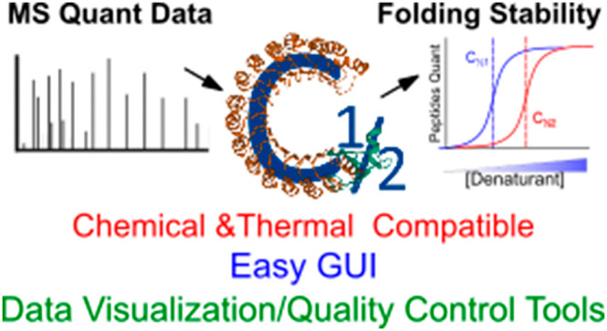
Abstract

The structure of a protein defines its function and integrity and correlates with the protein folding stability (PFS). Quantifying PFS allows researchers to assess differential stability of proteins in different disease or ligand binding states, providing insight into protein efficacy and potentially serving as a metric of protein quality. There are a number of mass spectrometry (MS)-based methods to assess PFS, such as Thermal Protein Profiling (TPP), Stability of Proteins from Rates of Oxidation (SPROX), and Iodination Protein Stability Assay (IPSA). Despite the critical value that PFS studies add to the understanding of mechanisms of disease and treatment development, proteomics research is still primarily dominated by concentration-based studies. We found that a major reason for the lack of PFS studies is the lack of a user-friendly data processing tool. Here we present the first user-friendly software, C_Half, with a graphical user interface for calculating PFS. Besides calculating site-specific PFS of a given protein from chemical denature folding stability assays, C_Half is also compatible with thermal denature folding stability assays. C_Half also includes a set of data visualization tools to help identify changes in PFS across protein sequences and in between different treatment conditions. We expect the introduction of C_Half to lower the barrier of entry for researchers to investigate PFS, promoting the usage of PFS in studies. In the long run, we expect this increase in PFS research to accelerate our understanding of the pathogenesis and pathophysiology of disease.

Introduction

In a physiological setting, a protein’s folding determines its structure and function and thus is integral to its proper biological application. As a result, the quality of a protein is directly related to the quality of its folding. Hence, changes in protein folding can negatively impact protein quality and can produce changes in cellular function that can lead to disease.¹ Most studies of disease and biomarkers, however, rely on measuring these downstream effects by using traditional proteomics methods to measure changes in concentrations of biomolecules which cannot quantify protein quality.² Measuring protein concentration changes may result in a diagnosis³ but frequently cannot actually quantify the biophysical causes of disease or whether a therapeutic interacts specifically with a protein of interest. Hence, nonconcentration-based methods are essential for diagnosing disease sooner and identifying potential treatment methods. Utilizing methods that quantify protein folding may provide more directly quantifiable information on causes of pathogenesis and pathophysiology, as well as provide direct evidence of therapeutic engagement with proteins of interest.

Consulting previous reviews of proteomic approaches to measuring protein stability,² there exists a range of in vivo, mass spectrometry (MS)-based methods that can probe protein folding using thermal denature approaches, such as Thermal Protein Profiling (TPP),⁴ or using chemical denature approaches such as Stability of Proteins from Rates of Oxidation (SPROX),⁵ and the Iodination Protein Stability Assay (IPSA).⁶ Each of these methods can measure differential stability of proteins in native and disease states, potentially providing insight into protein quality, by measuring protein folding stability (PFS). As protein structure is a function of PFS, physiologically significant insights can be made about in vivo protein quality by measuring PFS. By quantifying changes in PFS, such methods have proven able to identify drug-target interactions and to elucidate new potential drug targets.⁷ The PFS methods are widely applicable as they can probe stability changes at the level of individual amino acid residues or full-length proteins. Because these methods are MS-based, they also have high throughput and can measure changes in protein structure within complex mixtures and for many proteins simultaneously.

Despite these inherent advantages, PFS methods, however, have not been widely adopted. Some roadblocks for adoption may be a lack of familiarity with PFS methods within the proteomics community or the current heavy emphasis on concentration-based biomarker discovery methods. We also observed that there is a lack of a user-friendly, publicly available tools for calculating PFS from MS data (Table 1). Such a lack of tools, requires researchers to develop their own computational methods to calculate PFS and requires knowledge of programming in addition to an understanding of the nuances of PFS and structural biochemistry. This barrier to entry greatly limits the number of researchers who are able to experiment with PFS and limits the utilization of PFS as a subfield of proteomics.

Table 1. Literature Review of Tools for Calculating PFS^a.

Year	Publication	Language	Availability	GUI	Site PFSc	Visualization	PFS methodd
2022	H. Lin et al.6	Python	Public	Yes	Yes	Yes	Chem. and Therm.
2022	D. Childs et al.8b	R	Public	N/A	No	Yes	Them.
2022	E. Walker et al.9	Mathematica (Wolfram).	In house	N/A	N/A	N/A	Chem.
2021	N. McCracken et al.10	R	Public	N/A	N/A	Yes	Therm.
2021	Y. Xu et al.11	R	Public	N/A	N/A	N/A	Chem. and Therm.
2021	R. Ma et al.12	JAVA	In house	N/A	N/A	N/A	Chem.
2020	K. Lu et al.13	JAVA	In house	N/A	N/A	N/A	Chem.
2019	E. Walker et al.5	Mathematica (Wolfram).	In house	N/A	N/A	N/A	Chem.
2019	D. Childs et al.14	R	Public	N/A	No	Yes	Therm.
2018	H. Meng et al.15	Mathematica (Wolfram).	In house	N/A	N/A	N/A	Chem.

^aThe table lists known tools for calculating PFS. Details were extracted from the method sections of 9 publications and one public repository for the programs used to fit the sigmoid curve and calculate PFS.

^bFrom public repository.

^cLists if the program calculates the PFS of a given site of protein instead of peptide (discussed in depth in later sections).

^dChem. stands for chemical denature method and Therm. stands for thermal denature method.

To remedy this lack of publicly available tools for calculating PFS, we introduce C_Half, the first user-friendly software with a graphical user interface (GUI) for calculating PFS. Using C_Half requires no manipulation of the source code and facilitates measuring PFS through an easy-to-use graphical interface with customizable settings. Included with C_Half is a set of PFS data analysis and visualization tools useful for interpreting PFS data. C_Half can be used by veterans and newcomers to PFS alike and is a tool that can facilitate new research to bridge the apparent gap between concentration-based and structural approaches and perspectives to the study of disease.

Materials and Methods

In this section the modules of C_Half will be discussed. Three data sets were used for benchmarking the program: Lin et al.,⁶ for IPSA data, Walker et al.,⁵ for SPROX data, and Leijten et al.,¹⁶ for TPP data.

C_Half

C_Half is a publicly available tool written in Python compiled an executable available for download at https://github.com/JC-Price/CHalf_public/releases. Included with C_Half are instructions for installation and operation as well as a series of tutorial videos at https://github.com/JC-Price/Chalf_public#readme. C_Half requires an experimental design common to chemical or thermal denaturing experiments⁴⁻⁶ and that MS data be preprocessed through an MSMS identification and quantification software package such as Protein Prospector,¹⁷ Comet,¹⁸ Mascot,¹⁹ MaxQuant,²⁰ or PEAKS Studio.²¹Figure 1 shows the general workflow of C_Half from pre-C_Half processing (Figure 1A), C_Half Initialization (Figure 1B), curve fitting (Figure 1C), quality control tools (Figure 1D), combined site stability (Figure 1E), and data visualization (Figure 1F). Each step is discussed in detail in the following section.

Figure 1.

The workflow of C_Half. This figure maps the workflow of C_Half, shows the image of the GUI for each tool, and shows example visualization outputs. Each panel is a module in the program and leads to the next module. The blue text represents the input files required for the next module; the * represents the product output file from the referenced module; and the + represents the function that is excluded for thermal denature experiments. The full size of screenshot of the interface and output are included in Supporting Figure 2 for the details.

Data Pre-Processing

The C_Half tools were optimized to use PEAKS Studio proteins.csv and protein-peptides.csv output from the quantification module but can accept outputs from any other MS data analysis tools if formatted properly (Figure 1A). The input files should include peptide sequences, protein accessions/name, post-translational modification (PTM) annotated on the peptide sequence, quantified abundances that have had signal normalized to total ion count or similar methods across all the data files for the denaturation curve, peptide start and end positions in reference to the protein, and protein descriptions. Included in the documentation is an in-depth formatting guide for modifying quantification outputs from other MS data analysis tools and can be downloaded at https://github.com/JC-Price/Chalf_public/blob/main/Demos/CHalf%20Inputs%20Formatting%20Guide.xlsx.

Included as well is a tool for modifying quant outputs from MaxQuant or Proteome Discoverer to fit C_Half formatting requirements. These tools can be downloaded at https://github.com/JC-Price/Chalf_public/tree/main/CHalf%20Preprocesing%20Tools. For first time users, a practice set of C_Half inputs and outputs have also been included and can be downloaded at https://github.com/JC-Price/Chalf_public/tree/main/Example%20CHalf%20Files with included instructions.

C_Half Initialization

After inputs have been preprocessed, project and condition creation are facilitated using C_Half’s GUI (Figure 1B). Various project run settings can be modified using the C_Half Defaults file, accessible within the GUI. In a given C_Half project, multiple conditions with condition specific settings can be generated. Condition specific settings are modifiable using the condition creator GUI within C_Half. During condition creation, C_Half will also prompt data input. For an in-depth discussion of condition specific settings see “Heat/Chemical Denature” and “Curve Fitting”. After condition creation is complete, the project can be started, and progress can be monitored using a progress bar included in the C_Half output terminal.

Heat/Chemical Denature

C_Half can be used to calculate C_1/2 values from both thermal and chemical denaturation assays (Figure 2). Indicating the denaturation method in the condition allows C_Half to tailor its outputs in a method specific format.

• Concentrations/Temperatures Setting: When performing an assay to measure PFS, different denaturant types and gradients may be used to optimize for sample type and throughput or resolution. When creating a condition in C_Half, the gradient used is specified to allow for calculation of C_1/2 values. A preset gradient may also be specified in C_Half’s settings (Figure 1B).

Figure 2.

Experiment flow of protein folding stability (PFS) assay. (A) Chemical denature based PFS assay denature protein using denaturant like GdmCl or urea and then covalently modify the surface exposed amino acid residues. The labeled peptides serve as the probe for protein stability measurement. (B) Thermal denature based PFS assays denature protein using an increasing temperature gradient. The protein aggregates as the temperature increases. The soluble protein fraction serves as the probe for protein stability measurement.

Curve Fitting

As a protein is unfolded via chemical or thermal denaturation in a gradient, the fraction folded versus unfolded can be monitored by changes in relative protein/peptide abundances facilitated either by covalent labeling (like SPROX, IPSA) (Figure 2). or thermal protein aggregation (TPP). In both methods abundances are measured via MS quantification and used to calculate PFS using computational methods.

C_Half uses peptide abundances to calculate PFS by first normalizing them and plotting them against their denaturant concentration/temperature values (Figure 1C). These points are used to fit a sigmoid curve using the curve_fit method from the Python SciPy module²² and a fitting equation (eq 1) that has been used almost universally across different studies of PFS.⁴⁻⁶

1

The parameters for the equation were normalized peptide signal intensity in each fraction (y), final denaturant concentration or temperature of each fraction (x), pretransition baseline (A), post-transition baseline (B), denature midpoint (C_1/2 or T_m), and the slope of transition (b).

C_Half then measures PFS by identifying the point of inflection of the resulting sigmoid curve, known as the C_1/2 (or T_m) value. This value represents the concentration/temperature denaturation midpoint at which a given peptide or protein is found in a 1:1 ratio between its folded and unfolded state. This C_1/2 value represents the folding stability of the given protein or peptide and can be related to ΔG_unfolding through biophysical models.²³

Data is normalized across all samples in the curve prior to fitting using eq 1. Prior to the fit, data can be aggregated according to exact peptide sequences or using the specific chemical modification based on the relevant amino acid location in the protein (see “Site Specific C_1/2”). C_Half performs this curve fitting for all MS quantitated peptides, or sites in a sample and outputs curve data and C_1/2 values as.csv files for reference with an option of outputting graphics of each fitted curve (Figure 1C).

Replicates

For a condition of interest, biological or technical replicates may be used to increase the number of valid points for the calculation of C_1/2 values. Biological and/or technical replicates can help reduce the impact of random variation between runs and can increase the number of significant C_1/2 values measured in a sample. Replicates can be indicated within a C_Half condition using the condition creator GUI (Figure 1C).

• Individual Rep Analysis: When using multiple replicates, C_Half will generate reports for each individual replicate. Such reports can be used to identify potential error in replicates due to sample preparation or other confounding variables. This setting may also be turned off to reduce the time needed to perform C_1/2 calculations for a combined condition.

• Combined Analysis: When using multiple replicates, C_Half will combine replicates to produce sigmoid curves with more points, increasing the likelihood of generating fitting curves. This setting may also be turned off to reduce the time needed to perform calculations if only a single replicate is used. This setting however is necessary for “Remove Outlier Analysis” and is recommended regardless of the number of replicates used in a condition.

Remove Outlier Analysis

When calculating C_1/2 values, C_Half will attempt to use as many points as possible to generate fitting curves. Some measured values, however, may be inconsistent with the fitted curve and flagged as statistical outliers. Points are excluded if they are outside a range of two standard errors from the original fitted curve, and a second regression is performed using the new set of points. Using this setting allows C_Half to check for and remove statistical outliers to improve the accuracy of curve fitting. Evaluating the effect of C_Half’s outlier removal process, average R² values for fitting curves increased from 0.765 to 0.858 for the SPROX data set, indicating better fitting.

Quality Control

Inherent to any assay are issues such as noise or data scarcity. Data fitting is optimal when noise is low and data points are abundant. C_Half will attempt to fit curves to any amount of data and noise but tracks quality parameters such as R² values, confidence intervals, etc. for post-calculation quality control. C_Half includes a set of settings and tools for identifying and isolating significant data. Such tools are of great assistance in performing assay optimization, troubleshooting, and further data analysis workflows and visualization.

Minimum Points for Calculation

When calculating C_1/2 values, the number of valid points measured is essential to generating interpretable sigmoid curves. By default, C_Half requires a minimum of 4 valid points to generate sigmoid curves. This setting may be increased during condition creation to require more robust fitting conditions. If there are fewer nonzero points than the specified filter threshold, C_Half will not attempt to fit a curve for the peptide lacking sufficient points and will report the peptide as lacking a fitting curve. The number of points dramatically affects the fitting statistics. If we remove 4 data points (points 2, 4, 6, 8) from SPROX curves which originally had 9 points only 53% of the curves will pass the confidence requirements. Increased numbers of points help negate noise in the acquisition and improve the overall fit.

Label Finder (LF)

When performing chemical denaturation PFS assays, unfolding is measured via covalent labeling of solvent accessible amino acids. Many chemical modification methods exist for measuring PFS, but it is paramount across chemical denature methods to be able to track covalent modifications to measure PFS. Label Finder (LF) serves as a quality control tool for identifying assay labeling efficiency (Figure 1D).

Labeling efficiency is the ratio between peptides/proteins containing modified residues and modifiable residues. Identifying if the percentage of labeled proteins/peptides is within expected ranges is essential to assay method development and to identifying random error across runs. Whether or not a modifiable residue is labeled when fully exposed or if the labeled variant is detected in MS runs can be a function of kinetics, reaction equilibriums, MS ion suppression, etc.

LF measures labeling efficiency by identifying all proteins and peptides found in a given run that contain modifiable amino acid residues. It then counts the number of these modifiable peptides and proteins that have been labeled. Using this method, a 1:1 ratio between the counts of identified labeled peptide variants and nonlabeled peptides is the most optimal, providing a calculated labeling efficiency of 50%. Deviations from 50% labeling efficiency can be used to identify issues with reagents used in an assay, incubation times, or other confounding variables such as background labeling.

The LF defaults search for the PTM probes used for IPSA (Iodination (HY(+125.90)), Di-Iodination (HY(+251.79)), Oxidation (M(+15.99)), Sulphone (M(31.99)), Sulfenic Acid (C(+15.99)), Sulfinic Acid(C(+31.99)), and Sulfonic Acid (C(+47.98)), but can be easily changed according to the need of the user.

Fitting Efficiency

Fitting efficiency (FE) is the percentage of peptides which pass the fitting statistics filters compared to the total number of identified peptides. The FE is an essential metric for identifying the effectiveness of a run or assay for measuring PFS. When calculating PFS, C_Half will attempt to generate sigmoid curves for each peptide identified in MS runs. Insufficient data, an absence of change in relative abundances due to a lack of labeling or aggregation, or other inconsistencies can result in the generation of curves with fitting statistics. Such values do not provide meaningful data, so filtering out insignificant from significant curves is essential to data interpretation (Figure 1D).

C_Half’s FE tool performs data refinement by removing noisy points and serves as a quality control tool for optimizing assay or run fitting efficiency. Calculating fitting efficiency can also assist in troubleshooting individual runs through a stepwise reporting method that highlights at what calculation step filters reject sigmoid curves, providing insight into issues in a given run or method.

FE performs data refinement by checking that sigmoid curves provide C_1/2 values that are within reasonable ranges for the utilized PFS method, have acceptable R² values, and have reasonable confidence intervals that can be set by user in C_Half Defaults.csv. Included as well in FE is a second curve fitting step to combine same-residue-same-label-site peptide variants to isolate site-specific C_1/2 values for targetable residues. In its current iteration, C_Half does not adjust fitting efficiency percentages for method-specific targeted residues due to the wide range of method-specific targets, but future iterations will include presets for method specific analyses. Refined data from FE is output as a set of easy to use and nonproprietary .csv files that can be used later for data visualization or analysis by other tools and software.

Computing Site-Specific C_1/2

A challenge in the workflow for calculating C_1/2 values comes from cleavage patterns and measurement sensitivities inherent to proteomic assays and MS data acquisition. Oftentimes, many peptides containing the same chemically modified residue but different cleavage sites resulting in different peptide lengths are measured. These peptides can be analyzed individually or aggregated to calculate a site-specific PFS. As a result, C_Half is able to calculate and interpret PFS at a residue-specific level, increasing the resolution of chemical PFS assays (Figure 1E). This function is performed as part of C_Half’s FE tool. It should be noted, however, that site-specific C_1/2 calculations can only be performed on data using chemical modifications as the reporter in thermal aggregation methods is not site-specific.

C_Half Outputs and Post-C_Half Data Analysis

C_Half produces a series of .csv files containing folding curve metrics such as the C_1/2 value and curve quality metrics. Each step of C_Half and C_Half tools draws from subsets of data from former steps with the intent of isolating high-quality, interpretable data. The full workflow is explained in Figure 1. The most major outputs are Combined Outputs for thermal denature methods and Combined Label Sites for chemical labeling methods. A full discussion of all C_Half outputs and column names can be found at https://github.com/JC-Price/Chalf_public/blob/main/Demos/CHalf%20Outputs%20Explained.md.

Combined Outputs contain raw fitting data and C_1/2 values that can be filtered by users to isolate significant curves for use in identifying changes in folding stability due to experimental conditions in thermal denature experiments. The current version of FE does not isolate the subset of high-quality thermal denature curves as its isolation method is optimized for chemical labeling methods, but later versions will be further optimized for TPP specific run conditions. Data from Combined Outputs, however, can easily be sorted to isolate desired TPP data in Excel or other data manipulation tools. Further analysis can also easily be performed using user-defined pipelines.

Combined Label Sites files contain the subset of site-specific C_1/2 values that have passed all quality control checks. Combined Label Sites can be considered the ultimate output for chemical labeling methods and is hence used in most of C_Half’s data visualization tools. Data from Combined Label Sites can also easily be sorted and used in Excel or other data analysis tools for performing statistical tests.

C_Half is not intended to perform postfitting statistical analysis, or data interpretation. Statistical testing is best applied in an experiment and method specific manner. Hence, we do not attempt to perform statistical tests for comparing conditions in order to allow users to use best statistical practices when trying to analyze data and generate conclusions. C_Half’s purpose is to provide a user-friendly tool for calculating PFS from MS data and isolate high quality fitting curves in a format that can readily be used in user-made data analysis pipelines.

Visualization

Central to hypothesis generation and assessment is data interpretation. A challenge of working on a proteomic scale is quickly interpreting large data sets. As a result, large amounts of time are spent scouring data in search of trends. Much of this scouring can be streamlined through data visualization methods. C_Half includes a set of data visualization tools useful for making inferences into changes in PFS across experimental conditions as a result of changes in variables such as drug application. C_Half visualization tools are optimized for site-specific C_1/2 measurements, so some of the visualization, including CS, RM, and CRM, do not apply to workflows such as TPP. Graphing, however, may be applied to any PFS experiment workflow.

Graphing

Sigmoid curves generated by C_Half to calculate C_1/2 values may optionally be output as figures. Graphs are not automatically generated to reduce computation time, but individual replicate and combined condition graphs may be generated if specified in the condition creator. Settings for graph generation may also be applied to reduce computation time by limiting figure generation to more significant curves (Figure 1C).

• Format: The user can select figure output formats including .svg, .png, and.jpg.

• CI Mx% of Range (confidence interval percentage of range): By default, C_Half will only create graph figures for C_1/2 values that have confidence intervals that are within 30% of the range between the starting and ending denaturant concentrations/temperatures, reducing output size by limiting figure generation to more significant sigmoid curves. Changing this parameter will affect the number of figures generated by modifying the rigor necessitated to create figures.

• R² Cutoff: By default, C_Half will only output curve figures with R² values of 0.99 or above. Likewise, this parameter serves to reduce the number of generated figures to more significant sigmoid curves and reduces computational time and output file sizes.

• C_1/2 Range Cutoff: By default, C_Half will only output curve figures with C_1/2 or T_m values that are inside an interval of the minimum denaturant value minus 50% of the denaturant curve range and 50% of the range higher than the maximum denaturant value. This parameter also serves to limit generated figures to more significant sigmoid curves.

Combined Site (CS)

The goal of most any PFS experiment is to identify changes in PFS as a response to changes in other variables such as drug introduction. Combined Site (CS) is a data visualization tool included in C_Half that generates boxplots of measured C_1/2 values from same-label residue sites shared between conditions. This tool helps users to visually identify potentially significant changes in PFS as a result of changes in experimental conditions. Similarly, Combined Site outputs can help users to identify innate variation in PFS potentially caused by protein lability (Figure 1F). As a result, CS is a useful tool for identifying drug-target interactions and effects.

CS accepts C_Half’s combine label site.csv (Figure 1F) and outputs boxplot figures as well as a reference table containing the statistical information corresponding to the visualized data. As a tool, CS largely serves to help users quickly identify site specific variation. Quick identification of variation or lack of variation can help users to weigh current hypotheses, identify new potential hypotheses to test, and isolate specific data subsets to subject to more rigorous statistical methods.

Residue Mapper (RM)

Proteins can be composed of several subunits and regions that serve different purposes and have different functions. As protein function is determined by structure and folding, different regions of proteins will exhibit different PFS values with implications linked to function.²⁴ Identifying these differences in PFS may help identify structural information necessary to elucidating mechanisms of protein function and to identifying potential drug targets.

Residue Mapper (RM) helps visualize these differences in PFS across regions of proteins. Using C_Half combine label site.csv from FE module (Figure 1F), Residue Mapper generates figures plotting measured C_1/2 values against their residue numbers. These figures allow for users to quickly identify regions of stability and instability within a protein, providing insight into relative surface accessibility, and can potentially help with identifying ligand binding sites or other sites of interaction (Figure 1F).

Combined Residue Mapper (CRM)

When studying PFS, especially within physiological conditions, the goal of most any experiment is to identify methods useful for diagnosis or treatment of disease. Identifying changes in PFS as a result of variables such as disease or presence of drugs or other binding partners can potentially provide insight into the mechanisms by which diseases function, drugs interact with and stabilize proteins, and protein partners bind.²⁵

CRM serves to help visualize changes in PFS across regions of proteins in between different conditions. Similar to RM, CRM plots C_1/2 values against residue numbers for each condition allowing for quick interpretation of impacts of experimental variables on PFS throughout proteins, making global protein analysis of drug impacts faster and easier (Figure 1F).

CRM also generates a table report of all PFS measurements at sites across conditions called RCS summary. RCS summary can be used for quickly comparing stabilities between shared sites across conditions in further data analysis workflows and is generated in an easy to use, nonproprietary .csv format.

Results and Discussion

Here we demonstrate the application of C_Half to various studies of PFS using chemical or thermal denaturation methods including IPSA, SPROX,⁵ and TPP¹⁶ using C_Half version 4.2.1. Each study uses their respective method to measure changes in PFS due to drug or ligand binding. All data has been previously published and can be accessed in their respective Supporting Information sections. The MS raw data were all processed using PEAKs Studio and searched against Uniprot/SwissProt database (downloaded in October 2020) prior to C_Half analysis. C_Half was run using a Windows machine with 16 GB of RAM and a 2.6 GHz CPU. Run results are presented in Table 2, and significant findings are discussed below. C_Half outputs, specific run conditions, and detailed specifications of the machine used can be found in the supplemental packages 1, 2, 3, and 4.

Table 2. C_Half Run Results.

	IPSA		SPROX		TPP
Sample	Purified Transferrin		Fibroblast Cells		Zebrafish Embryo Lysate
Condition	Apo	Holo	Control	TMAO	Control	NB
#Repliates	3	3	3	1	1	1
Peptide IDs	292	400	68,925	27,776	12,635	13,212
Protein IDs	9	32	4,984	2,972	1,101	1,257
PEPTIDE Label Efficiency	55.65%	47.68%	53.93%	36.58%	N/A	N/A
RAW PEPTIDE Fitting Efficiency	29.45%	28.25%	12.77%	8.67%	37.77%	75.41%
aMethod Specific Peptide Fitting Efficiency	18.35%	14.65%	21.17%	10.44%	37.77%	75.41%
Fitted Label Sites	51	52	3718	715	N/A	N/A
Combined Label Sites	36	40	3214	669	N/A	N/A
Shared Sites between Conditions	13		329		N/A
Condition Prep Time	1 min. 30 s		1 min. 10 s		3 min. 20 s
Total Runtime w/o graphic output	43 s		37 min. 18 s		12 min. 56 s

^aMethod Specific Peptide Fitting Efficiency refers to the percentage of peptides with high quality fitting curves that are measurable by the specific method compared to the total number of peptides that are probable by that method. For example, SPROX method specific fitting efficiency refers to the ratio of fitting curves containing methionine residues to all peptides containing methionine residues.

Additionally, we compare analysis performed by C_Half to that of existing software to compare user-friendliness and data processing quality.

IPSA Findings

Transferrin (TF) is a transport protein known to bind iron at 2 lobes. TF with iron bound at both lobes (Holo) has been shown to be more stable than unbound TF (Apo).²⁶ Lin et al. use IPSA to examine this difference in PFS between purified Apo and Holo TF. Although this study showed that the assay could be used in complex mixtures like the blood serum the comparison of the purified protein is especially useful to demonstrate the full suite of C_Half tools to quickly provide insight into changes in PFS as a result of ligand binding.

Combined Site (CS) identified 13 shared sites between Apo and Holo and generated site-specific figures for each. CRM generated figures highlighting PFS differences between Apo and Holo. CRM suggested increases in TF stability associated with iron binding consistent with literature findings, where the holoTF is more stable than apoTF.²⁶ (Figure 3A). Using RCS summary.csv from C_Half, we generated scatterplots to examine the global effects of iron binding on PFS between labeled sites shared between both Apo and Holo conditions (Figure 3B). Results suggest a general increase in stability of Holo when comparing to, consistent with the reports of Lin et al.

Figure 3.

C_Half graphic result from sample data set. (A–C) The graphic results of IPSA experiment. (D–F) The graphics results of SPROX experiment. For the IPSA and SPROX experiments, a combined site figure for a given label site of a protein is shown on the left column, and the combined residue mapper (the middle column) shows the site C_1/2 across a protein’s sequence. (G–I) The graphic results of a TPP experiment. Since the TPP experiment does not label specific site of a protein, the denature curves are used to show the treatment effect on the same peptide. The scatter plot of site C_1/2 or peptide T_m (the right column) is used to show the global PFS change due to ligand binding or drug treatment.

SPROX Findings

Walker et al. use SPROX to examine the difference in PFS between untreated control fibroblast cell lysate (Control) and fibroblast cell lysate treated with a chemical chaperone known to stabilize proteins, trimethylamine N-oxide (TMAO).⁵ We demonstrate the use of C_Half to process their quantitated MS data and quickly provide insight into changes in PFS as a result of drug treatments.

Combined site (CS) identified 13 shared sites between Control and TMAO and generated site-specific figures for each CRM generated figures highlighting PFS differences between Control and TMAO. CRM suggested increases in most proteins’ stabilities associated with TMAO application (Figure 3C). Using RCS summary.csv from C_Half, we generated scatterplots to examine the global effects of TMAO application on PFS between oxidized sites shared between both Control and TMAO conditions (Figure 3D). All results suggest a general increase in stability between Control and TMAO, consistent with the reports of Walker et al.

TPP Findings

Leijten et al. use TPP to examine PFS in untreated control zebrafish embryo cell lysate (Control) and zebrafish embryo cell lysate treated with a drug, napabucasin (NB).¹⁶ We demonstrate the use of C_Half to process their quantitated MS data and quickly generate unfolding curves to get insight into PFS using TPP data. The analysis of the TPP data was essentially the same as the IPSA and SPROX data except that no amino acid modifications were included in the initial preprocessing steps, thus there are no CS, RM, CRM outputs. To illustrate the change of PFS due to treatment, we used C_Half to generate thermal denature curves for comparison (Figure 3E). All curves were negative as shown in Figure 2B in contrast to the IPSA and SPROX curves which were predominately positive (Figure 2A). Using combined output.csv from C_Half of the two conditions, we also generated scatterplots to examine the global effects of NB application on PFS (Figure 3F). Results suggested that global effects were largely insignificant.

Software Comparisons

C_Half serves as a tool to simplify the data processing requirements for researchers interested in studying PFS. As such, C_Half was designed to be user-friendly and widely applicable to analysis of all PFS assays. As a result, C_Half can perform PFS analysis on both chemical labeling and thermal denature methods, unlike previous programs. To compare C_Half with existing software for PFS determination, we repeated the data analysis described above using publicly available PFS software and the same data inputs from the C_Half runs (discussed above) to provide a benchmark for comparison. To the best of our knowledge, there are no publicly available programs for the calculation of PFS for chemical labeling methods. Hence, no comparison could be made. There exist, however, publicly available programs for thermal denature PFS calculation. We used Inflect¹⁰ to measure PFS values using inputs from the same Leijten et al.¹⁶ TPP data to allow a direct comparison of the software.

Inflect was installed in an R environment, and C_Half’s input file was adapted to fit Inflect’s input format. Analysis was then performed in an R terminal, yielding TPP PFS curves. Following discussion will focus on comparing the user experience and analysis results of Inflect to C_Half.

Regarding user experience, operating Inflect also required familiarity with R. Inflect required the download of the R programming language project, required the download of several library dependencies, and had to be operated from an R compatible IDE. Adapting quantification data to the input format of Inflect, however, was relatively easy, and the outputs generated were intuitive.

In comparison, C_Half can be downloaded as an executable, requiring no additional dependencies for installation, can be operated using a user-friendly, intuitive GUI rather than a command line. This reduces the requirement for programming experience and provides tools for adapting quant outputs to be used as C_Half inputs. Hence, C_Half is easier to adopt and use, and C_Half provides a unique contribution to PFS measurement software.

Regarding analysis, C_Half and Inflect utilize different curve fitting methods. C_Half utilizes a more traditional curve fitting eq (eq 1), whereas Inflect utilizes its own logistic fitting method optimized for TPP as described in its release paper.¹⁰ Both methods have been shown to produce useful PFS curves but do not produce the same quality control metrics to allow for complete direct comparison. Comparing the results yielded from both programs with comparable quality control metrics (curves with C_1/2 values within the range of 34 and 64 degrees and having an R² value of greater than 0.6), C_Half produced 8237 curves compared to Inflect, producing 6968 curves. Applying other C_Half-specific confidence interval quality control metrics, C_Half yielded 6257 curves. Hence, we anticipate that Inflect’s curve fitting method may be more stringent but ultimately comparable when utilizing additional C_Half-specific quality control measures.

Regarding other features, Inflect is optimized for TPP whereas C_Half is not. Hence, Inflect outputs are very useful for examining differential curves observed in TPP. C_Half approaches PFS data from single point C_1/2 values with confidence intervals, meaning it produces more interpretable PFS data for chemical modification methods. Such a method can also be applied to TPP data, but differential curve methods are potentially superior for TPP.

Overall, C_Half is widely applicable, being able to process both chemical and thermal data, and is simpler to use and adopt than existing PFS software. Similarly, C_Half produces interpretable PFS data that is comparable to existing software.

Conclusion

Traditional concentration-based proteomic approaches can provide unique insight into disease and human health through biomarker discovery but do not adequately factor in changes in protein quality. PFS methods possess the ability to combine strengths from both structural biology and proteomics and introduce a new dimension to the study of human health by providing a quantitative measure of protein quality. Hence, the combination of methods can provide a complete framework to fully describe pathogenesis and pathophysiology. Understanding the biophysical roots of disease is a critical first step to identifying new drug targets and better methods of diagnosis.

PFS, however, has been largely neglected due to high barriers of entry associated with a lack of computational tools. We present C_Half in an effort to remove these barriers and to provide the opportunity for any researcher to introduce the dimension of protein quality to their experiments’ workflows. It has been demonstrated that C_Half is an easy to use and efficient tool. C_Half reduces barriers to studying PFS in a variety of ways: (1) C_Half is publicly available and has a user interface designed to be simple to use to reduce difficulty of adoption and streamline inputting data; (2) C_Half uses a computationally light calculation method, allowing for efficient calculation of PFS from most any computer; (3) C_Half includes a host of easy-to-modify settings that allow users to easily include C_Half in their workflow; options to adjust C_Half for denature and labeling methods can be tailored to any PFS assay; (4) C_Half inputs can be created from a variety of MSMS analysis tools, and outputs are nonproprietary filetypes easily used by user defined data analysis tools including Excel and most bioinformatics tools; (5) C_Half documentation includes an expanding list of video tutorials and explanations to ease adoption. Beyond easy adoptability, C_Half has a growing number of features to aid in data analysis and visualization which ease data interpretation and figure preparation. As advances are made in PFS, we aim to continue to expand this list of features to further increase the use that C_Half and PFS can provide to the study of human health and disease.

The express aim of C_Half is to make including PFS elements into proteomic studies as simple as possible. Removing barriers to studying PFS are essential to increasing PFS’s adoption within proteomics and to incorporating a new potential dimension to the study of disease. We expect C_Half to greatly ease entrance into the study of PFS and to aid in a potentially fruitful union of structural biology and proteomic approaches to the study of disease.

Supporting Information Available

The Supporting Information is available free of charge at https://pubs.acs.org/doi/10.1021/acs.jproteome.2c00619.

• Supporting Table 1 - Machine Specifications for C_Half runs, Supporting Figure 1 – C_Half Specific Run Conditions, Supporting Figure 2 – C_Half Program interface in Figure 1 (PDF)

• Supporting Material 1-C_Half Projects Directory Organization and File Descriptions – Map of file directories for C_Half projects with annotations for identifying filetypes (XLSX)

• Supporting Material 2-IPSA C_Half Project – The output files from the application of C_Half to IPSA workflow (ZIP)

• Supporting Material 3-SPROX C_Half Project – The output files from the application of C_Half to SPROX workflow (ZIP)

• Supporting Material 4-TPP C_Half Project – The output files from the application of C_Half to TPP workflow (ZIP)

Author Contributions

⁺ C.D.H. and H.-J.L.L. contributed equally to this work.

The authors declare no competing financial interest.

References

- Outeiro T. F.; Tetzlaff J. Mechanisms of Disease II: Cellular Protein Quality Control. Seminars in Pediatric Neurology 2007, 14 (1), 15–25. 10.1016/j.spen.2006.11.005. [DOI] [PubMed] [Google Scholar]
- Kaur U.; Meng H.; Lui F.; Ma R.; Ogburn R. N.; Johnson J. H. R.; Fitzgerald M. C.; Jones L. M. Proteome-Wide Structural Biology: An Emerging Field for the Structural Analysis of Proteins on the Proteomic Scale. J. Proteome Res. 2018, 17 (11), 3614–3627. 10.1021/acs.jproteome.8b00341. [DOI] [PMC free article] [PubMed] [Google Scholar]
- Drucker E.; Krapfenbauer K. Pitfalls and limitations in translation from biomarker discovery to clinical utility in predictive and personalised medicine. EPMA Journal 2013, 4 (1), 7. 10.1186/1878-5085-4-7. [DOI] [PMC free article] [PubMed] [Google Scholar]
- Franken H.; Mathieson T.; Childs D.; Sweetman G. M. A.; Werner T.; Tögel I.; Doce C.; Gade S.; Bantscheff M.; Drewes G.; et al. Thermal proteome profiling for unbiased identification of direct and indirect drug targets using multiplexed quantitative mass spectrometry. Nat. Protoc. 2015, 10 (10), 1567–1593. 10.1038/nprot.2015.101. [DOI] [PubMed] [Google Scholar]
- Walker E. J.; Bettinger J. Q.; Welle K. A.; Hryhorenko J. R.; Ghaemmaghami S. Global analysis of methionine oxidation provides a census of folding stabilities for the human proteome. Proc. Natl. Acad. Sci. U. S. A. 2019, 116 (13), 6081–6090. 10.1073/pnas.1819851116. [DOI] [PMC free article] [PubMed] [Google Scholar]
- Lin H.-J. L.; James I.; Hyer C. D.; Haderlie C. T.; Zackrison M. J.; Bateman T. M.; Berg M.; Park J.-S.; Daley S. A.; Zuniga Pina N. R.; et al. Quantifying In Situ Structural Stabilities of Human Blood Plasma Proteins Using a Novel Iodination Protein Stability Assay. J. Proteome Res. 2022, 21, 2920. 10.1021/acs.jproteome.2c00323. [DOI] [PMC free article] [PubMed] [Google Scholar]
- Jiawen L.; Keyun W.; Mingliang Y. Modification-free approaches to screen drug targets at proteome level. TrAC Trends Anal. Chem. 2020, 124, 115574. 10.1016/j.trac.2019.06.024. [DOI] [Google Scholar]
- Childs D.; Kurzawa N.; Franken H.; Doce C.; Savitski M.; Huber W.. TPP: Analyze thermal proteome profiling (TPP) experiments; Bioconductor, 2022; 10.18129/B9.bioc.TPP. [DOI]
- Walker E. J.; Bettinger J. Q.; Welle K. A.; Hryhorenko J. R.; Molina Vargas A. M.; O’Connell M. R.; Ghaemmaghami S. Protein folding stabilities are a major determinant of oxidation rates for buried methionine residues. J. Biol. Chem. 2022, 298 (5), 101872 10.1016/j.jbc.2022.101872. [DOI] [PMC free article] [PubMed] [Google Scholar]
- McCracken N. A.; Peck Justice S. A.; Wijeratne A. B.; Mosley A. L. Inflect: Optimizing Computational Workflows for Thermal Proteome Profiling Data Analysis. J. Proteome Res. 2021, 20 (4), 1874–1888. 10.1021/acs.jproteome.0c00872. [DOI] [PMC free article] [PubMed] [Google Scholar]
- Xu Y.; West G. M.; Abdelmessih M.; Troutman M. D.; Everley R. A. A Comparison of Two Stability Proteomics Methods for Drug Target Identification in OnePot 2D Format. ACS Chem. Biol. 2021, 16 (8), 1445–1455. 10.1021/acschembio.1c00317. [DOI] [PubMed] [Google Scholar]
- Ma R.; Johnson J. H. R.; Tang Y.; Fitzgerald M. C. Analysis of Brain Protein Stability Changes in Mouse Models of Normal Aging and α-Synucleinopathy Reveals Age- and Disease-Related Differences. J. Proteome Res. 2021, 20 (11), 5156–5168. 10.1021/acs.jproteome.1c00653. [DOI] [PMC free article] [PubMed] [Google Scholar]
- Lu K.-Y.; Quan B.; Sylvester K.; Srivastava T.; Fitzgerald M. C.; Derbyshire E. R. Plasmodium chaperonin TRiC/CCT identified as a target of the antihistamine clemastine using parallel chemoproteomic strategy. Proc. Natl. Acad. Sci. U. S. A. 2020, 117 (11), 5810–5817. 10.1073/pnas.1913525117. [DOI] [PMC free article] [PubMed] [Google Scholar]
- Childs D.; Bach K.; Franken H.; Anders S.; Kurzawa N.; Bantscheff M.; Savitski M. M.; Huber W. Nonparametric Analysis of Thermal Proteome Profiles Reveals Novel Drug-binding Proteins*. Molecular & Cellular Proteomics 2019, 18 (12), 2506–2515. 10.1074/mcp.TIR119.001481. [DOI] [PMC free article] [PubMed] [Google Scholar]
- Meng H.; Ma R.; Fitzgerald M. C. Chemical Denaturation and Protein Precipitation Approach for Discovery and Quantitation of Protein–Drug Interactions. Anal. Chem. 2018, 90 (15), 9249–9255. 10.1021/acs.analchem.8b01772. [DOI] [PubMed] [Google Scholar]
- Leijten N. M.; Bakker P.; Spaink H. P.; Den Hertog J.; Lemeer S. Thermal Proteome Profiling in Zebrafish Reveals Effects of Napabucasin on Retinoic Acid Metabolism. Molecular & Cellular Proteomics 2021, 20, 100033. 10.1074/mcp.RA120.002273. [DOI] [PMC free article] [PubMed] [Google Scholar]
- Baker P. R.; Clauser K. R.. Protein Prospector. https://prospector.ucsf.edu/ (accessed 2022).
- Eng J. K.; Jahan T. A.; Hoopmann M. R. Comet: An open-source MS/MS sequence database search tool. PROTEOMICS 2013, 13 (1), 22–24. 10.1002/pmic.201200439. [DOI] [PubMed] [Google Scholar]
- Mascot. http://www.matrixscience.com/search_form_select.html (accessed 2022).
- Cox J.; Mann M. MaxQuant enables high peptide identification rates, individualized p.p.b.-range mass accuracies and proteome-wide protein quantification. Nat. Biotechnol. 2008, 26 (12), 1367–1372. 10.1038/nbt.1511. [DOI] [PubMed] [Google Scholar]
- PEAKS Studio. https://www.bioinfor.com/peaks-studio/ (accessed 2022).
- SciPy. https://scipy.org/ (accessed 2022).
- Lin H.-J. L.Quantifying Protein Quality to Understand Protein Homeostasis; Brigham Young University, Provo, UT, 2022. https://scholarsarchive.byu.edu/etd/9618?utm_source=scholarsarchive.byu.edu%2Fetd%2F9618&utm_medium=PDF&utm_campaign=PDFCoverPages. [Google Scholar]
- Batey S.; Nickson A. A.; Clarke J. Studying the folding of multidomain proteins. HFSP Journal 2008, 2 (6), 365–377. 10.2976/1.2991513. [DOI] [PMC free article] [PubMed] [Google Scholar]
- Broglia R. A.; Serrano L.; Tiana G.. Protein Folding and Drug Design; IOS Press, 2007. [Google Scholar]
- Alina K.; Sowmya I.; Pernille S.; Lorenzo G.; Werner S.; Dierk R.; Wolfgang F.; Günther H. J. P.; Pernille H. Small angle X-ray scattering and molecular dynamic simulations provide molecular insight for stability of recombinant human transferrin. J. Struc. Biol.: X 2020, 4, 100017 10.1016/j.yjsbx.2019.100017. [DOI] [PMC free article] [PubMed] [Google Scholar]
Associated Data
This section collects any data citations, data availability statements, or supplementary materials included in this article.