Simultaneous hypothesis testing for multiple competing risks in comparative clinical trials

Abstract

Competing risks data are commonly encountered in randomized clinical trials or observational studies. Ignoring competing risks in survival analysis leads to biased risk estimates and improper conclusions. Often, one of the competing events is of primary interest and the rest competing events are handled as nuisances. These approaches can be inadequate when multiple competing events have important clinical interpretations and thus of equal interest. For example, in COVID-19 in-patient treatment trials, the outcomes of COVID-19 related hospitalization are either death or discharge from hospital, which have completely different clinical implications and are of equal interest, especially during the pandemic. In this paper we develop nonparametric estimation and simultaneous inferential methods for multiple cumulative incidence functions (CIFs) and corresponding restricted mean times. Based on Monte Carlo simulations and a data analysis of COVID-19 in-patient treatment clinical trial, we demonstrate that the proposed method provides global insights of the treatment effects across multiple endpoints.

1 |. INTRODUCTION

Randomized clinical trials are frequently designed to determine effective interventions with respect to time-to-event outcomes. For standard time-to-event data, restricted mean survival times, defined as the mean failure time up to a pre-specified time point, $\tau$, and estimated as the area under survival curve, have been increasingly used to characterize failure time distribution and compare between treatment groups (Chen & Tsiatis;¹ Karrison;² Royston & Parmar;^3,4 Zhang & Schaubel;⁵ Andersen et al;⁶ Uno et al⁷). More recently, restricted mean times are also proposed to characterize the cumulative incidence function of a particular failure subject to competing risks (Anderson⁸).

Competing risks data are frequently encountered in clinical research, where individuals may experience one of two or more different types of events (failures), and the occurrence of any event precludes the occurrences of the other event types. In cancer research, for example, time to cancer-related death is often of primary interest, where deaths due to comorbidities and natural causes naturally constitute competing risks. As a competing event prevents the occurrence of the primary event of interest, special attention and methodology are required to obtain unbiased estimation and inference. Much of competing risks literature, for example, Putter et al⁹ and references within, concerns competing risks data when one of the event type is of primary interest. These approaches treat the other competing events as nuisances in data analysis. For example, when comparing the cancer-related deaths between treatments, existing methods, such as Gray’s method,¹⁰ properly handle non-cancer deaths in background.

There are, however, situations where multiple event types are all of interest simultaneously. As an illustrative example, let us consider RCTs evaluating optimal treatments for hospitalized patients who were infected with SARS-CoV-2 and diagnosed as COVID-19. After patients were admitted to hospitals and treated, their ending status of hospitalization would be either death or discharge from hospital due to recovery. As discussed by McCaw et al,¹¹ recovery and death naturally constitute competing risks: one’s occurrence precludes the occurrence of the other and patients’ ending status could remain unknown at the time of interim or final analysis, especially for those experiencing prolonged hospitalization. In this case, the competing events (death or recovery) have complete different clinical interpretations. During a pandemic when healthcare resources are stressed, analysis of either death or recovery alone, by treating the other as nuisance, can hardly reveal a complete story nor allow us to decisively conclude whether the experimental regimen should be used in the future.

Additional examples also arise in cardiovascular or oncology trials, where composite endpoints, such as time to the first of any major adverse cardiac event (MACE: such as cardiovascular death or nonfatal acute myocardial infarction) or disease-free survival (DFS: time to the first of local recurrence, distant metastasis, secondary cancer or all-cause death), are used frequently. These composite endpoints, when specified carefully in appropriate contexts, may increase the statistical precision and thus the trial efficiency. Meanwhile, it is often concerned that novel interventions do not necessarily impact all components of a composite endpoint equally. For example, when evaluating the role of extended adjuvant endocrine therapy for early-stage breast cancers (Mamounas et al¹²), the extended treatment is only expected to improve breast cancer-specific outcomes, but not non-breast cancer deaths. In fact data shows that, with longer follow-up, the relative contribution of non-breast death to defining events of DFS increases. Taken together, using DFS as the primary endpoint could result in less, rather than more, statistical power to detect any putative treatment effect, because improvements in breast cancer-specific outcomes would be “diluted” by the contribution of non-breast cancer deaths. Moreover, if a composite endpoint, such as time to MACE, consists of both short-term safety and long-term efficacy components, a unidirectional tally would obscure or even distort the underlying benefit-risk assessment.¹³ In all of these cases, simultaneously assessing all components of a composite endpoint would be highly desirable.

In presence of competing events, cumulative incidence function (CIF) plays a fundamental role in competing risks data analysis. It describes the probability of experiencing one particular type of failure over time, and can be estimated nonparametrically by, for example, Aalen-Johansen estimator.¹⁴ In data analysis, CIFs for each event type can be particularly useful for different stakeholders. For example, when we are at the peaks of a pandemic and healthcare resources are stressed, CIF of hospital discharge and patient recovery is of great interest to health administration and public health researchers; meanwhile physicians and patients might focus more on the disease progression and thus find the CIF of death more relevant. Nonetheless, when more than one failure event is available and of equal interest, it is highly desirable to develop joint inference approach for two or more CIF estimators so that practitioners can simultaneously characterize different aspects of the disease progression and evaluate optimal treatment. Li and Yang¹⁵ developed joint inferential methods for cause-specific hazard (CSH) functions and CIFs of survival times subject to competing risks. They also introduced a number of testing statistics for the simultaneous comparison of CSH functions and CIFs, as well as joint regression analyses of CSHs and CIFs. In contrast, as we shall demonstrate in this paper, we concentrate on nonparametric testing methods based on CIFs, the corresponding restricted mean times, and composite measures of restricted mean times of multiple competing events. Of note, one important and unique contribution of our work studies a composite measure of restricted mean times of multiple CIFs. Such a composite measure, which is built on functional transformation of multiple CIFs, can flexibly assess the benefit-risk trade-off across different competing events, a feature that was not considered by methods developed by Li and Yang.¹⁵

Furthermore, when measuring the treatment effect, most time-to-event analyses heavily rely on hazard ratio from the proportional hazards model.¹⁶ Among the many issues of using hazard-based approaches to analyze competing risks data, one of them is that the hazard ratio for one endpoint may not be sufficient to fully characterize the putative benefits of the intervention. For example, considering the rapid development of COVID-related morbidity and mortality, a reduction in mortality hazard could be equivalent to prolong the survival a few days under intensive care, which by itself may be insufficient to justify a practice change. Restricted mean survival time (RMST) has been increasingly considered lately to alternatively quantify the failure time distribution. In this paper, we will demonstrate how to use restricted mean times for multiple competing events to globally quantify their distributions.

In summary, in this paper we develop estimation methods and joint inferential results of multiple CIFs and its related metrics. With an emphasis on competing risks data with two failure types, the proposed methods collectively address the unmet needs of comparing treatment groups by incorporating multiple disease outcomes. The remainder of this paper is organized as follows. Section 2 studies nonparametric estimators of CIFs and related large sample properties of their joint distributions. Section 3 introduces restricted mean time for competing risks and their use for simultaneous inference. Section 4 provides several testing statistics for two-sample comparison under restricted mean time framework. Section 5 evaluates the operating characteristics of proposed methods through Monte Carlo simulations and Section 6 presents data analysis from a COVID-19 comparative clinical trial. Section 7 provides concluding remarks and some further directions.

2 |. JOINT INFERENCE OF MULTIPLE CUMULATIVE INCIDENCE FUNCTIONS

2.1 |. Background review

This section develops joint inference of nonparametric estimators of multiple CIFs. Denote by $T$ the time to a failure event, and assume the failure time variable $T$ is continuous with distribution function (d.f.) $F\left(t\right)$, survival function $S_T\left(t\right)=P\left(T\ge t\right)$, and hazard function $\lambda \left(t\right)$. Let the censoring time be denoted by $C$, which has continuous d.f. $G\left(t\right)$ and survival function $S_C\left(t\right)=P\left(C\ge t\right)$. Denote by $\Delta =I\left(T\le C\right)$ the censoring indicator, $X=min\left(T,C\right)$ the observed failure time, and $\eta$ the type of failure which takes value $1,2,\cdots ,J$. Then the observed data can be described as $\left(X_i,{\Delta }_i{\eta }_i\right),i=1,2,\cdots ,n$. Assume the independent censoring condition holds; that is, $T$ is independent of $C$.

The cumulative incidence function for type-j risk is $F_j\left(t\right)=P\left(T\le t,\eta =j\right)$. The cause specific hazard function for type-j risk is ${\lambda }_j\left(t\right)$, where ${\lambda }_j\left(t\right)dt=d{F}_j\left(t\right)/S_T\left(t\right)$. Let $H$ represent the distribution function for $X$, and further define the sub-distribution functions $H^j\left(t\right)=P\left(X\le t,\Delta \eta =j\right)$. Therefore $H^j\left(t\right)$ is the distribution function for type-j uncensored failure time. The cumulative incidence function for type-j risk can then be expressed as

$$F_j\left(t\right)=P\left(T\le t,\eta =j\right)=\underset{0}{\overset{t}{\int }}\frac{d{H}^j\left(u\right)}{1-G\left(u\right)}=\underset{0}{\overset{t}{\int }}{S}_T\left(u\right)\frac{d{H}^j\left(u\right)}{1-H\left(u\right)}du$$

We estimate the overall survival function $S_T(\cdot )$ by Kaplan-Meier estimator ${\hat{S}}_T(\cdot )$, distribution function $H$ by ${\hat{H}}_n\left(t\right)=$ ${\sum }_{i=1}^{n}I\left(X_i\le t\right)/n$ and sub-distribution function $H^j\left(t\right)$ by ${\hat{H}}_n^j\left(t\right)={\sum }_{i=1}^{n}I\left(X_i\le t,{\Delta }_i{\eta }_i=j\right)/n$, then the Aalen-Johansen estimator can be given by

$${\hat{F}}_j\left(t\right)=\underset{0}{\overset{t}{\int }}\frac{{\hat{S}}_T\left(u\right)}{1-{\hat{H}}_n\left(u\right)}d{\hat{H}}_n^j\left(u\right)$$

By martingale theory and the functional delta method, asymptotic normality properties of a single CIF estimator has been studied by Bryant & Dignam,¹⁷ Lin¹⁸ and Zhang & Fine.¹⁹ Under Assumptions (1) and (2) in the Appendix, $\sqrt{n}\{{\hat{F}}_j\left(t\right)-F_j\left(t\right)\}$ converges weakly to a zero-mean Gaussian process $V_j\left(t\right)$, in which with for all $t,s>0$,

$$cov\left\{V_j\left(t\right),V_j\left(s\right)\right\}=\underset{0}{\overset{s\wedge t}{\int }}\frac{\left\{F_j\left(t\right)-F_j\left(u\right)\right\}\left\{F_j\left(s\right)-F_j\left(u\right)\right\}}{S_T\left(u\right)S_C\left(u\right)}\lambda \left(u\right)du+\underset{0}{\overset{s\wedge t}{\int }}\frac{S_T\left(u\right)-\left\{F_j\left(t\right)+F_j\left(s\right)-2F_j\left(u\right)\right\}}{S_C\left(u\right)}{\lambda }_j\left(u\right)du$$

The variance of $V_j\left(t\right)$ can be estimated using the observed data by

$$\underset{0}{\overset{t}{\int }}\frac{1}{Y{(u)}^2}\left({\left\{{\hat{F}}_j\left(t\right)-{\hat{F}}_j\left(u\right)\right\}}^{2}dN\left(u\right)+\left[{\hat{S}}_T{(u)}^2-2{\hat{S}}_T\left(u\right)\left\{{\hat{F}}_j\left(t\right)-{\hat{F}}_j\left(u\right)\right\}\right]d{N}_j\left(u\right)\right)$$

in which ${\hat{S}}_T\left(t\right)$ is the Kaplan-Meier estimator for overall survival function, ${\hat{F}}_j\left(t\right)$ is the Aalen-Johansen estimator for the cumulative incidence function for type-j risk, $N\left(t\right)={\sum }_{i=1}^n{N}_i\left(t\right)={\sum }_{i=1}^{n}I\left(X_i\le t,{\Delta }_i{\eta }_i\ne 0\right)$ is the total number of uncensored failure events prior to time $t,N_j\left(u\right)={\sum }_{i=1}^n{N}_{ij}\left(t\right)={\sum }_{i=1}^{n}I\left(X_i\le t,{\Delta }_i{\eta }_i=j\right)$ is the total number of uncensored type-j failure event priors to time $t$, and $Y\left(t\right)={\sum }_{i=1}^n{Y}_i\left(t\right)={\sum }_{i=1}^{n}I\left(X_i\ge t\right)$ denotes the total number of subjects at risk at time $t$.

2.2 |. Joint asymptotic distribution of two CIF estimators

Simultaneous evaluation of multiple CIFs relies on the joint distribution of multiple CIFs. Without loss of generality, as described in Andersen et al,²⁰ the joint asymptotic distribution of two CIF estimators, ${\hat{F}}_j\left(t\right)$ and ${\hat{F}}_k\left(t\right),1\le j<k\le J$, can be summarised in the proposition below.

Proposition 1. Under Assumptions (1)-(3), which are described in the Appendix, $\sqrt{n}{\left[\left\{{\hat{F}}_j\left(t\right)-F_j\left(t\right)\right\},\left\{{\hat{F}}_k\left(t\right)-F_k\left(t\right)\right\}\right]}^T$ converges weakly to a bivariate Gaussian process ${\left\{V_j\left(t\right),V_k\left(t\right)\right\}}^T$. That is, for all $t,s>0$,

$$\left(\begin{array}{c}{V}_j\left(t\right)\\ V_k\left(s\right)\end{array}\right)~𝒩\left(\overrightarrow{0},\left(\begin{array}{cc}{\sigma }_{jj}^2\left(t\right)& {\sigma }_{jk}\left(t,s\right)\\ {\sigma }_{kj}\left(s,t\right)& {\sigma }_{kk}^2\left(s\right)\end{array}\right)\right),$$

in which ${\sigma }_{jj}^2\left(t\right),{\sigma }_{jk}\left(t,s\right),{\sigma }_{kj}\left(s,t\right)$ and ${\sigma }_{kk}^2\left(s\right)$ can be found in the Appendix.

Following from the linearity of normal distribution, all linear transformations of the two CIF estimators will automatically converge weakly to a Gaussian process and these properties can be used to find the asymptotic distributions of statistics constructed from multiple CIFs.

3 |. JOINT INFERENCE OF RESTRICTED MEAN TIMES

3.1 |. Restricted mean time for competing risks

Using COVID-19 in-patient RCTs as a motivating example, because recovery and death are two mutually exclusive ending status of hospitalization, they can be naturally considered as competing events. By denoting recovery (hospital discharge) and death as competing event type $1\left(\eta =1\right)$ and type $2\left(\eta =2\right)$, we can define

$${\mu }_1=\text{E}\left[\left\{\tau -T\right\}\times I\left(\eta =1,T\le \tau \right)\right]=\underset{0}{\overset{\tau }{\int }}{F}_1\left(t\right)dt,$$

$${\mu }_2=\text{E}\left[\left\{\tau -T\right\}\times I\left(\eta =2,T\le \tau \right)\right]=\underset{0}{\overset{\tau }{\int }}{F}_2\left(t\right)dt,$$

where $\tau$ is the pre-specified timepoint to end the trial. In COVID-19 example, ${\mu }_1$ and ${\mu }_2$ are thus interpreted as restricted mean time gained (due to discharge, RMTG) or restricted mean time lost (due to death, RMTL), respectively. In contexts outside of COVID-19 in-patient trials, interpretations of ${\mu }_1$ and ${\mu }_2$ may be defined accordingly.

Figure 1 illustrates the relationship of cumulative incidences of competing events and corresponding restricted mean times (ie, RMTG and RMTL), where $\tau$ is pre-specified at 28 days. The lower curve in Figure 1 is the cumulative incidence function (CIF) of time to death, and the area underneath between 0 and day 28 (left-shaded area) is RMTL. The upper curve in the figure is the sum of CIFs of time to death and time to recovery, and the area between two curves (right-shaded area) corresponds to RMTG. The remaining area on left upper portion can be interpreted as the restricted mean time spent in hospital. The RMTG and RMTL are two key summary measures that directly correspond to recovery and death and characterize patients’ disease development and eventual outcomes. The mean time of hospitalization is a direct measure of healthcare resource utilization, irrespective to treatment outcome.

FIGURE 1.

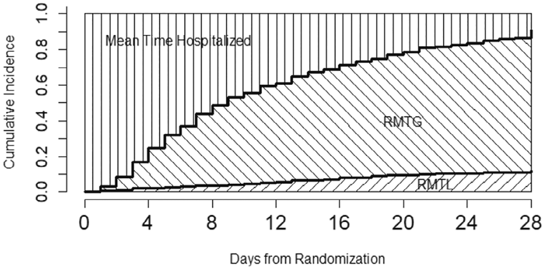
Restricted mean time gained (RMTG) and restricted mean time lost (RMTL).

3.2 |. Combining multiple restricted mean times of competing risks

The estimation of restricted mean time of each competing event, such as RMTG and RMTL, can be easily constructed using Aalen-Johansen’s estimation approach.¹⁴ For $j=1,2$, a straightforward estimator is ${\hat{\mu }}_j={\int }_0^{\tau }{\hat{F}}_j\left(t\right)$. Using the results in Proposition 1 (Section 2), large sample properties of ${\hat{\mu }}_j,j=1,2$ are given in the theorem below.

Theorem 1. Under Assumptions (1)-(3) in the Appendix, $\sqrt{n}{\left\{{\hat{\mu }}_1-{\mu }_1,{\hat{\mu }}_2-{\mu }_2\right\}}^T$ has an asymptotically bivariate normal distribution with mean 0 and variance-covariance matrix $\Sigma =\left({\sigma }_{ij}\right)$ as $n\to \infty$, where ${\sigma }_{ij},i,j=1,2$ can be found in the Appendix.

In COVID-19 clinical trials, an ideal intervention is expected to have a large RMTG $\left({\mu }_1\right)$ and small RMTL $\left({\mu }_2\right)$ in the treatment group. As discussed in Section 1, when multiple competing events are of interest, interpretations rely on any of competing events alone may fail to provide us a full picture of the disease progression and treatment evaluation. Therefore, to allow concrete interpretation and facilitate evidence synthesis, we propose to construct a “composite” efficacy measure using multiple CIFs and their corresponding restricted mean times:

$$\mathbf{\Psi }=a+b{\mu }_1+c{\mu }_2=\underset{0}{\overset{\tau }{\int }}a+b{F}_1\left(t\right)+c{F}_2\left(t\right)dt$$

in which $a,b,c$ are pre-specified weights or utilities and chosen by investigators and stakeholders. By plugging in the Aalen-Johansen estimators for the CIFs ${\hat{F}}_j$, we can give a nonparametric estimator $\hat{\mathbf{\Psi }}$.

The choice of pre-specified weight $\left(a,b,c\right)$ reflects the stakeholders’ considerations of how to balance benefits and risks, and thus should be tailored based on disease and treatment settings. In COVID-19 trials, as an example, when choosing $\left(a,b,c\right)=\left(0,1,-1\right)$, the efficacy measure $\mathbf{\Psi }$ corresponds to the “net” restricted mean time gained (RMTG – RMTL), which directly reflects the “net benefits” of a given COVID-19 regimen. As another example, we may define a treatment efficacy measure using a linear combination of three areas (mean time hospitalized, RMTG, RMTL) in Figure 1: $a^{\text{*}}\left\{\tau -{\mu }_1-{\mu }_2\right\}+b^{\text{*}}{\mu }_1+c^{\text{*}}{\mu }_2$, which is equivalent to $\mathbf{\Psi }=a+b{\mu }_1+c{\mu }_2$, where $a=a^{\text{*}}\times \tau ,b=b^{\text{*}}-a^{\text{*}},c=c^{\text{*}}-a^{\text{*}}$. Note that $a^{\text{*}}=0$ (or $a=0$) means the trial effect does not take into account the mean time in hospital. In general, the size of $a,b,c$ determines how much investigators care about the three areas. For example, if they want to emphasize on the death rate, they should set the absolute value of $c$ to be much larger than that of $b$ so that RMTL plays a bigger role. More detailed discussion on the choice of pre-specified $\left(a,b,c\right)$ is beyond the scope of this paper, as their choice should be context-specific and reflect the stakeholder’s benefit-risk consideration.

In settings where composite endpoints, such as DFS in breast cancer, are used, $\mathbf{\Psi }$ becomes the difference between $\tau$ and restricted mean survival time of DFS when taking $\left(a,b,c\right)=\left(0,1,1\right)$. When a quantitative benefit-risk assessment is of interest, additional choices of $\left(a,b,c\right)$ may be desired and solicited through the use of a survey tool and a modified Delphi panel consisting of clinician investigators with experience in randomized controlled trials. Such an approach has been implemented in cardiovascular diseases by Armstrong et al²¹ in order to derive a weighted composite endpoint, time to first any major adverse cardiac event (MACE).

Based on asymptotic properties of the restricted mean time for each competing event, as described in Theorem 1, the asymptotic normality property of their linear combination, $\hat{\Psi }$, is given in Theorem 2 below.

Theorem 2. Under Assumptions (1)-(3) in the Appendix, $\hat{\Psi }$ satisfies $\sqrt{n}\left(\hat{\Psi }-\Psi \right)\stackrel{D}{\to }N\left(0,{\sigma }^2\right)$, in which ${\sigma }^2$ can be found in the Appendix.

Based on the large sample result described in Theorem 2, hypothesis testing statistics can be developed to evaluate the intervention efficacy in clinical trials if a composite measure is of interest. We will describe such statistics for two-sample comparison in Section 4.3.

4 |. JOINT HYPOTHESIS TESTING FOR MULTIPLE RESTRICTED MEAN TIMES

Here we develop inference results to test two restricted mean times of competing events, for example, RMTL and RMTG, simultaneously in two-sample setting. We consider a typical RCT with two independent groups of subjects, and the competing risks of interest are subject to independent censoring, with possibly different censoring distributions for each group. Let ${\mu }_{1k},{\mu }_{2k}$ denote RMTG and RMTL in group $k,k=1,2$ for control and treatment, respectively. Further denote ${\hat{s}}_{1k},{\hat{s}}_{ck},{\hat{s}}_{2k}$ the estimated variance of RMTG, the estimated covariance between RMTG and RMTL, the estimated variance of RMTL in group $k,k=1,2$, respectively. We develop nonparametric tests for the following joint null hypothesis:

$$H_0:{\mu }_{11}={\mu }_{12}\text{ and }{\mu }_{21}={\mu }_{22}$$

4.1 |. Chi-square joint test

Define

$$X^2=\left({\hat{\mu }}_{11}-{\hat{\mu }}_{12},{\hat{\mu }}_{21}-{\hat{\mu }}_{22}\right){\Sigma }_c^{-1}\left(\begin{array}{l}{\hat{\mu }}_{11}-{\hat{\mu }}_{12}\hfill \\ {\hat{\mu }}_{21}-{\hat{\mu }}_{22}\hfill \end{array}\right)$$

in which

$${\Sigma }_c=\left(\begin{array}{ll}{\hat{s}}_{11}+{\hat{s}}_{12}\hfill & {\hat{s}}_{c1}+{\hat{s}}_{c2}\hfill \\ {\hat{s}}_{c1}+{\hat{s}}_{c2}\hfill & {\hat{s}}_{21}+{\hat{s}}_{22}\hfill \end{array}\right)$$

Under null hypothesis $H_0,X^2$ has an asymptotically chi-square distribution with two degrees of freedom. This leads to the following chi-square test for $H_0$ : Reject $H_0$ at level $\alpha$ if $X^2>{\chi }_2^2\left(\alpha \right)$, where ${\chi }_2^2\left(\alpha \right)$ is the upper $1-\alpha$ percentile of the standard ${\chi }_2^2$ distribution.

4.2 |. Maximum joint test

Define

$$T^{\text{*}}=max\left(\left|Z_1\right|,\left|Z_2\right|\right)$$

in which $Z_1=\left\{{\hat{\mu }}_{11}-{\hat{\mu }}_{12}\right\}/\sqrt{{\hat{s}}_{11}+{\hat{s}}_{12}}$ and $Z_2=\left\{{\hat{\mu }}_{21}-{\hat{\mu }}_{22}\right\}/\sqrt{{\hat{s}}_{21}+{\hat{s}}_{22}}$. It follows from Theorem 1 above that for large samples, the distribution of $\left(Z_1,Z_2\right)$ can be approximated by the bivariate normal distribution $N\left({(0,0)}^T,{\Sigma }_T\right)$, where ${\Sigma }_T=\left(\begin{array}{ll}1\hfill & \rho \hfill \\ \rho \hfill & 1\hfill \end{array}\right)$ and $\rho =\left({\hat{s}}_{c1}+{\hat{s}}_{c2}\right)/\sqrt{\left({\hat{s}}_{11}+{\hat{s}}_{12}\right)\left({\hat{s}}_{21}+{\hat{s}}_{22}\right)}$. Therefore, we can derive the distribution of $T^{\text{*}}$ using resampling methods. Specifically, we generate $\text{N}$ pairs of random variables from the bivariate normal distribution $N\left({(0,0)}^T,{\Sigma }_T\right)$. For each pair, we compute the maximum, denoted by $T_i^{*},i=1,2,\cdots ,N$. Let $T_{\alpha }$ be the upper $100(1-\alpha )$ th sample quantile of $T_1^{\text{*}},\cdots ,T_N^{\text{*}}$ and we reject the null hypothesis $H_0$ at level $\alpha$ if $T^{\text{*}}>T_{\alpha }$.

4.3 |. Test of composite efficacy measure

As elaborated in Section 3.2, one may be interested in comparing a “composite” efficacy measure using multiple CIFs and their corresponding restricted mean times between two arms in RCTs, where the composite measure is defined as

$$\mathbf{\Psi }=a+b{\mu }_1+c{\mu }_2=\underset{0}{\overset{\tau }{\int }}a+b{F}_1\left(t\right)+c{F}_2\left(t\right)dt$$

A comparison between ${\hat{\mathbf{\Psi }}}_1$ and ${\hat{\mathbf{\Psi }}}_2$, where the subscripts indicating the treatment/control group from a RCT, provides an immediate quantitative “benefit-risk” assessment. For example, we can construct a Z test statistic as following

$$Z=\frac{\left|{\hat{\mathbf{\Psi }}}_1-{\hat{\mathbf{\Psi }}}_2\right|}{\sqrt{{\hat{\sigma }}_1^2+{\hat{\sigma }}_2^2}}$$

We will be convinced there is significant difference between the two groups at level $\alpha$ if $Z>Z\left(1-\alpha /2\right)$, where $Z\left(1-\alpha /2\right)$ is the upper $1-\alpha /2$ percentile of the standard normal distribution. The details of estimated ${\hat{\mathbf{\Psi }}}_k$ and ${\hat{\sigma }}_k^2$, for $k=1,2$ can be found in Appendix.

5 |. MONTE CARLO SIMULATION STUDIES

Monte Carlo simulations are used to evaluate the operating characteristics of the proposed tests in a typical RCT, comparing a new treatment (Arm 2) to control (Arm 1) with 1:1 randomization ratio. Motivated by the breast cancer trial (Mamounas et al¹²) and COVID-19 treatment trial introduced in Section 1, we focus on situations where two competing event types are observed and of interest simultaneously. In these cases, analytic and interpretation challenges may arise when differential treatment effects may be expected on different failure types. We therefore consider two scenarios: Scenario I represents cases similar to breast cancer trials, where the two competing events are possibly correlated and components of a composite endpoint (eg, DFS), meanwhile the treatment effect is only postulated in one of failure types; Scenario II represents situations similar to COVID-19 treatment trials, where a negative correlation between the failure types is plausible.

In Scenario I, we apply the simulation procedures described in Beyersmann et al²² to simulate competing risks data under arbitrary underlying relationship. That is, within each group, we start with postulating the cumulative incidence functions $F_1\left(t\right),F_2\left(t\right)$, for failure type 1 and 2 respectively, so that the corresponding cause-specific hazard function ${\lambda }_1\left(t\right)$, ${\lambda }_2\left(t\right)$ can be derived. The failure time $T$ is simulated based on the all cause hazard ${\lambda }_1\left(t\right)+{\lambda }_2\left(t\right)$, with a binomial selection probability ${\lambda }_1\left(t\right)/\left\{{\lambda }_1\left(t\right)+{\lambda }_2\left(t\right)\right\}$ to determine if it is failure type 1. As shown in Figure 2, we focus on a setting where the new treatment has a lower cumulative incidence of failure type 1, but similar cumulative incidence of failure type 2 as compared to control. In detail, for Group I, the CIFs are given by $F_1\left(t\right)=0.15\times \left\{1-\text{exp}\left(-t\right)\right\}$ and $F_2\left(t\right)=0.85\times \left\{1-\text{exp}\left(-0.5t\right)\right\}$. For Group II, the CIFs are given by $F_1\left(t\right)=0.2\times \left\{1-\text{exp}\left(-2t\right)\right\}$ and $F_2\left(t\right)=0.8\times \left\{1-\text{exp}\left(-0.6t\right)\right\}$.

FIGURE 2.

Underlying cumulative incidences: Scenario I & II.

In Scenario II, we focus on a negatively correlated competing risks data structure like COVID-19 trials, where the new treatment has no benefit on failure type 1 (eg, recovery) but does on type 2 (eg, mortality), as shown in Figure 2. In order to explicitly postulate a negative correlation between competing events, within each group, we simulate bivariate latent failure times, each following an exponential distribution marginally with own hazard rate, and use a Gaussian copula²³ to induce a negative correlation between the two failure times. Their pairwise minimum leads to the uncensored competing risks data, with association summarized in terms of Pearson’s correlation coefficient. In detail, for Group I, ${\lambda }_1=0.2,{\lambda }_2=0.5$ while for Group II, ${\lambda }_1=0.2,{\lambda }_2=1$, and the negative correlation is set to be −0.3 both.

For both scenarios, independent censoring is introduced through a random variable following uniform distribution, and calibrated to achieve a 20% censoring rate. We evaluate the proposed joint tests in terms of the empirical probabilities of rejecting (ie, “power”) the joint null hypothesis $(H_0:{\mu }_{11}={\mu }_{12}$ and ${\mu }_{21}={\mu }_{22})$, and compare them with tests comparing individual cumulative incidences of failure type $1\left(H_0^1:{\mu }_{11}={\mu }_{12}\right)$ and failure type $2\left(H_0^2:{\mu }_{21}={\mu }_{22}\right)$. To provide a contextual assessment across hypothesis tests, only RMT-based tests are considered. In addition, combinations of multiple RMT of competing events are compared accordingly $\left(H_0^C:{\psi }_1={\psi }_2\right)$ : in Scenario I, we compare $\mathbf{\Psi }$ with $\left(a,b,c\right)=c\left(0,1,1\right)$, that is, the sum of RMT for failure type 1 and 2; in Scenario II, we compare $\mathbf{\Psi }$ with $\left(a,b,c\right)=c\left(0,1,-1\right)$, that is, the “net” restricted mean time gained.

Based on 1000 simulation replicates, Figures 3 and 4 summarizes the empirical probabilities of rejecting the respective null hypotheses at $\alpha =0.05$ (one sided for joint tests, two sided for $\text{Z}$ tests) based on different $\tau$ values, when the sample sizes are $n=100,200,300$ (per arm). To evaluate the size of our proposed tests under global null, we simulate Group I data in Scenario II with sample size $n=100,200,300$. As shown in Figure 3, the joint tests and Z test all control the type I error rate well under all sample sizes as expected. Figure 4 shows the power analysis results under Scenario I and II, respectively. In Scenario I, where the treatment reduces the cumulative incidence of failure type 1 but not type 2, the probability of rejecting $H_0^1$ is highest while that of rejecting $H_0^2$ is lowest, as expected. In Scenario II, the probability of rejecting $H_0^2$ becomes the highest because the treatment only reduces the cumulative incidence of failure type 2. In both scenarios, the probabilities of rejecting $H_0$ with the proposed chi-square joint test and maximum joint test are both slightly lower than the highest rejection probability, as one would anticipate based on either $H_0^1$ or $H_0^2$, and far higher than that of testing the other failure type. The rejection probabilities of the joint tests are also higher than that of $H_0^C$ in both scenarios, suggesting the joint tests may be more sensitive in detecting meaningful differences across all competing events simultaneously than efforts combining competing events. In Scenario I, rejection probability of chi-square joint test is slightly higher than that of maximum joint test as $\tau$ gets larger, probably because a small but incremental benefit in failure type 2 only contributes to the chi-square joint test but not maximum test.

FIGURE 3.

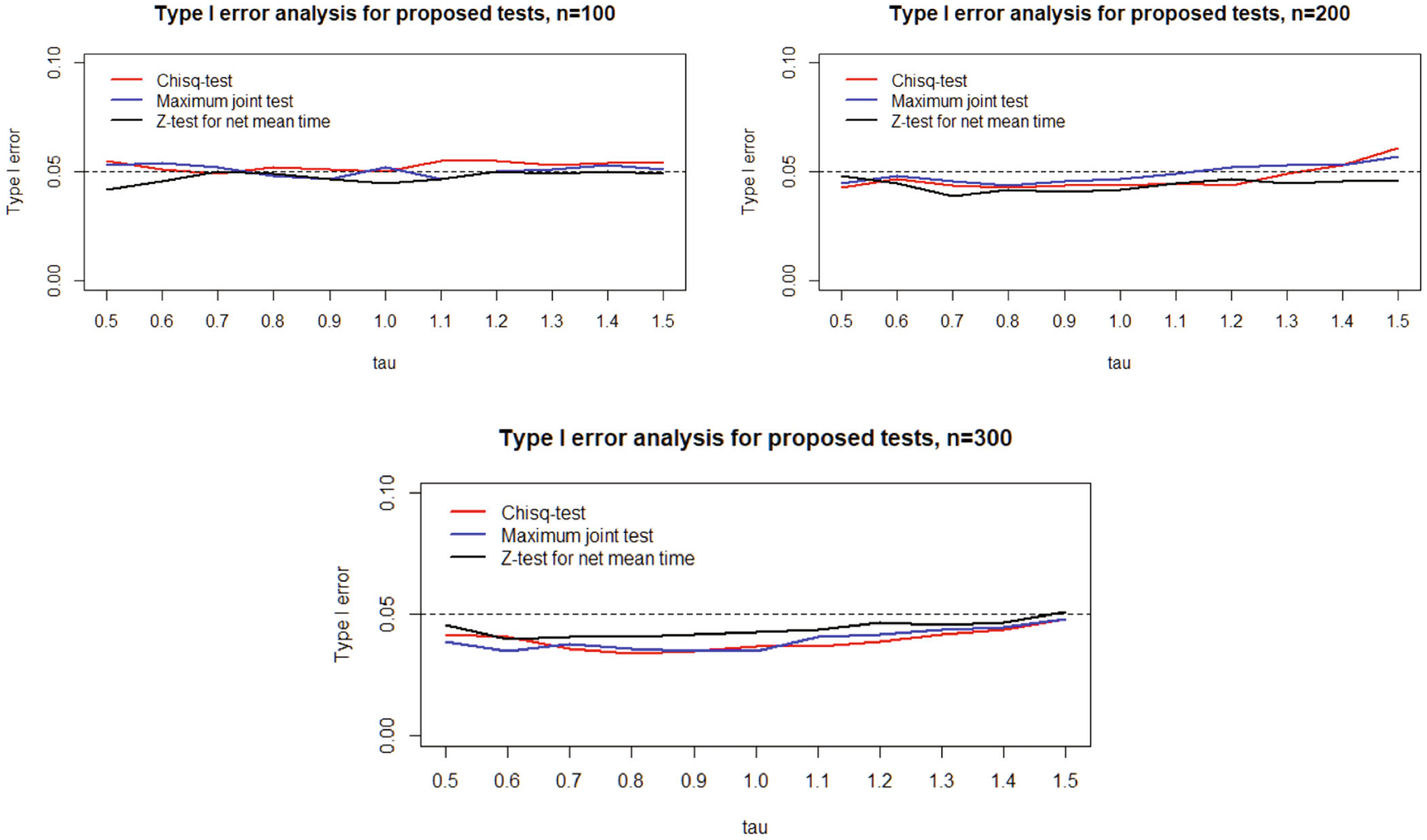
Type I error analysis of proposed tests.

FIGURE 4.

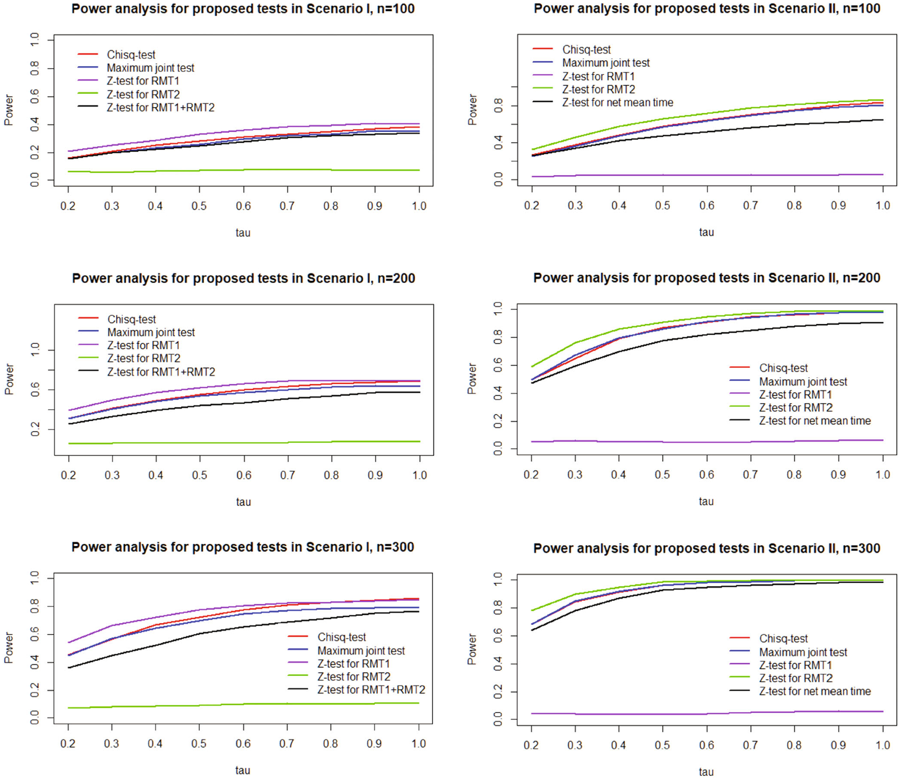
Power analysis of proposed tests.

6 |. DATA ANALYSIS: ADAPTIVE COVID-19 TREATMENT TRIAL

To further illustrate how to use the proposed joint tests to supplement competing risks analysis, we present a re-analysis of Adaptive COVID-19 Treatment Trial (ACTT-1). This is a double-blind, randomized, placebo-controlled phase III trial to evaluate intravenous remdesivir in adults who were hospitalized with COVID-19 and had evidence of lower respiratory tract infection. The details of study design, conduct, and pre-planned analysis results, including those based on standard survival analysis methods, can be found in Beigel et al.²⁴ In summary, using pre-specified standard survival analysis methods, the study found that remdesivir significantly accelerated time to recovery, while the mortality rate was significantly reduced only for time interval 1 ~ 15 days but not for 1 ~ 29 days. For illustration purposes, out of the 1062 randomized patients, we exclude 18 patients who withdrew consent early with no follow-up or longitudinal information, as well as 4 patients who died after hospital discharge. Our analysis thus consists of 528 on remdesivir arm and 512 on placebo arm. In this setting of hospitalized COVID-19 treatment evaluation, 15 and 29 days post admission (randomization) were chosen a priori given their clinical relevance. Of note, because a stratified test of proposed joint inference framework is beyond the scope of this paper, the presented results below are based on unadjusted analyses, which may result in wider confidence intervals and a reduction in power.²⁵

Using standard CIFs and the asymptotic variance estimators derived, we report restricted mean time gained and lost (RMTG and RMTL), evaluated up to $\tau =15$ and 29 Days, for both arms and respectively. Figure 5 visualizes the RMTG and RMTL in each group. Complementary to competing risks analysis of either recovery or death, the estimated differences in RMTG or RMTL between arms can be used for treatment comparisons, with Z-test for respective hypothesis testing. As shown in Table 1, the estimated restricted mean time gained (RMTG) due to recovery is significantly longer in remdesivir (1.366 days longer [95% CI: 0.798–1.934] over 15 days, and 2.743 days longer [95% CI: 1.552–3.933] over 29 days, $p<0.001$ for both), consistently confirm that remdesivir indeed accelerated recovery. Meanwhile, the estimated restricted mean time lost (RMTL) due to morality is significantly reduced by 0.427 days (95% CI: 0.127–0.727, $p=0.005$) over 15 days and 0.912 days (95% CI: 0.154–1.668, $p=0.018$) over 29 days. In contrast, based on standard survival analysis, the hazard ratio of mortality between remdesivir and placebo was 0.73 (95% CI, 0.52 to 1.03), and 0.55 (95% CI, 0.36 to 0.83) when limiting to first 15-day follow-up.

FIGURE 5.

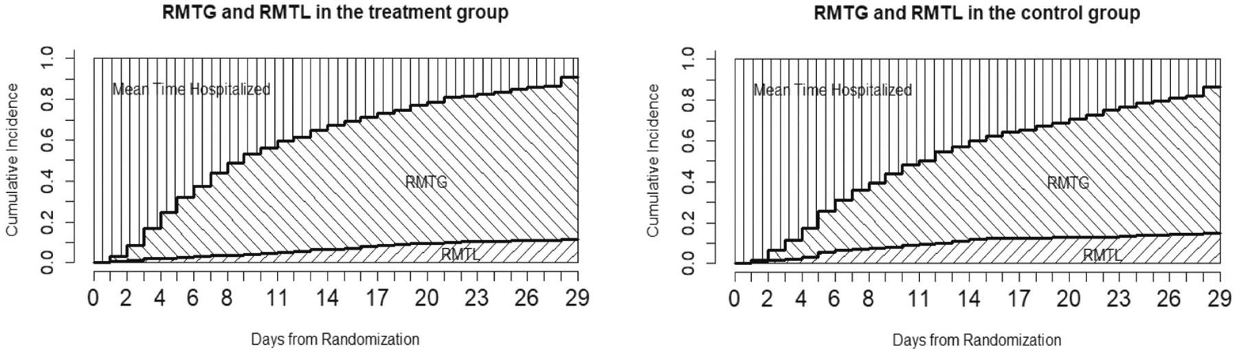
RMTG/RMTL plot in the two arms.

TABLE 1.

Restricted mean time analysis in ACTT-1 study.

	Treatment group (days)	Control group (days)
Day 15
Restricted mean time lost (RMTL)	0.521 (0.342–0.700)	0.948 (0.708–1.188)
Difference (95% CI)	0.427 (0.127–0.727), p-value = 0.005
Restricted mean time gained (RMTG)	5.254 (4.843–5.665)	3.888 (3.496–4.281)
Difference (95% CI)	1.366 (0.798–1.934), p-value < 0.0001
“Net” mean time gained (RMTG-RMTL)	4.733 (4.249–5.216)	2.940 (2.432–3.448)
Difference (95% CI)	1.793 (1.091–2.494), p-value < 0.0001
Chi-square joint test	${\chi }^2=\mathbf{25.246}$, p-value < 0.0001
Maximum joint test	$T^{*}=\mathbf{4.712}$, p-value < 0.0001
Day 29
Restricted mean time lost (RMTL)	1.896 (1.429–2.364)	2.808 (2.212–3.403)
Difference (95% CI)	0.912 (0.154–1.668), p-value = 0.018
Restricted mean time gained (RMTG)	15.094 (14.261–15.928)	12.351 (11.502–13.201)
Difference (95% CI)	2.743 (1.552–3.933), p-value < 0.0001
“Net” mean time gained (RMTG-RMTL)	13.198 (12.070–14.326)	9.543 (8.309–10.778)
Difference (95% CI)	3.655 (1.982–5.327), p-value < 0.0001
Chi-square joint test	${\chi }^2=\mathbf{20.537}$, p-value < 0.0001
Maximum joint test	$T^{*}=\mathbf{4.516}$, p-value < 0.0001

As argued earlier, it may be of interest to evaluate the “net” restricted mean time gained (nRMTG) $\mathbf{\Psi }$, by subtracting RMTL from RMTG, and compare it between arms as an alternative “benefit-risk” evaluation. We found nRMTG is significantly longer in remdesivir than placebo when evaluated over either the first 15 days (4.733 vs. 2.940 days, $p<0.001$) or 29 days (13.198 vs. 9.543 days, $p<0.001$), which also supports the use of remdesivir.

Lastly, we apply the proposed joint tests to determine if RMTG and RMTL between the remdesivir and control arm are equal at the same time. As shown in Table 1, Chi-square joint test and maximum joint test both suggest strong evidence to reject the null hypothesis, with p-value < 0.0001.

7 |. DISCUSSION

In this paper, we consider joint inference for multiple cumulative incidence functions under competing risks settings. Based on this, an analytical plan based on restricted mean times for comparative clinical trials is also developed. Asymptotic theory of the proposed estimators and corresponding testing methods are developed, which perform well in finite samples based on Monte Carlo simulations. The proposed methods are especially useful when two or more competing events are of equal interest, have opposite clinical interpretations.

As we argue, the joint inference tools for multiple CIFs as well as associated restricted mean times are expected to provide intriguing global insights to physicians, patients and health administrators to facilitate their decision-making. The proposed methods have wide applications in multiple sub-disciplines in medicine. In addition to COVID-19 treatment trials, a putative negative correlation and opposite interpretations between competing events also naturally arise in critical care (Resche-Rigon et al²⁶) and epileptic seizure (Williamson et al²⁷) clinical research. Furthermore, cardiovascular and cancer research frequently consider a combination of disease-related nonterminal events and death as key primary and secondary endpoints. A simultaneous assessment for multiple competing events could be particularly desirable to better understand the global impacts on the disease natural history by new treatments.

From study design perspective, a joint inference framework presumably provides an opportunity to reduce sample sizes and increase power by detecting difference in CIF of any competing event, which is a topic of future research. In addition, it is well known that covariate adjustment, while generally increases estimation precision in linear models, is not necessarily the case in non-linear models. In the context of competing risks data, it would be of interest to investigate if adjusting baseline prognostic factors may increase estimation precision of restricted mean times of competing events.

An important topic of restricted mean survival time literature is the choice of evaluation time $\tau$. Generally speaking, for comparative studies, its choice should be pre-specified at design stage and based on clinical considerations. Tian et al²⁸ showed that a data-dependent choice of $\tau$, based on the smaller of the largest follow-up time (either observed or censored) in both arms, is also justifiable under relatively mild condition of censoring distribution. We anticipate a similar argument is likely held in competing risks and applied to our proposal, although additional investigations are surely warranted to better understand the impacts of $\tau$ in both design and analysis of RCT.

APPENDIX A. REGULARITY CONDITIONS

The regularity conditions used in the theorems are as follows:

1. The censoring time $C$ is independent of survival time $T$ and failure type $\eta$.

2. The distribution of $C$ and $T$ are continuous.

3. One subject can only fail due to only one type of cause at certain time, which is, denote $N_{ij}\left(t\right)=I\left(X_i\le t,\Delta \eta =j\right)$ to count subject $i$ type-j failure event prior to time $t$, then $P\left\{d{N}_{il}\left(s\right)=1,d{N}_{ik}\left(s\right)=1\right\}=0$ for any $s$ and $l\ne k$.

APPENDIX B. VARIANCE/COVARIANCE COMPONENTS IN THE PROPOSITIONS/THEOREMS

B.1. Proposition 1

$${\sigma }_{jj}^2\left(t\right)=\underset{0}{\overset{t}{\int }}{\left\{F_j\left(t\right)-F_j\left(u\right)\right\}}^2\frac{1}{S_T\left(u\right)S_C\left(u\right)}\lambda \left(u\right)du+\underset{0}{\overset{t}{\int }}\frac{S_T\left(u\right)-2\left\{F_j\left(t\right)-F_j\left(u\right)\right\}}{S_C\left(u\right)}{\lambda }_j\left(u\right)du,$$

$${\sigma }_{kk}^2\left(s\right)=\underset{0}{\overset{s}{\int }}{\left\{F_k\left(s\right)-F_k\left(u\right)\right\}}^2\frac{1}{S_T\left(u\right)S_C\left(u\right)}\lambda \left(u\right)du+\underset{0}{\overset{s}{\int }}\frac{S_T\left(u\right)-2\left\{F_k\left(s\right)-F_k\left(u\right)\right\}}{S_C\left(u\right)}{\lambda }_k\left(u\right)du,$$

$${\sigma }_{jk}\left(t,s\right)={\sigma }_{kj}\left(s,t\right)=\underset{0}{\overset{s\wedge t}{\int }}\frac{\left\{F_j\left(t\right)-F_j\left(u\right)\right\}\left\{F_k\left(s\right)-F_k\left(u\right)\right\}}{S_T\left(u\right)S_C\left(u\right)}\lambda \left(u\right)du-\underset{0}{\overset{s\wedge t}{\int }}\left\{F_k\left(s\right)-F_k\left(u\right)\right\}\frac{1}{S_C\left(u\right)}{\lambda }_j\left(u\right)du-\underset{0}{\overset{s\wedge t}{\int }}\left\{F_j\left(t\right)-F_j\left(u\right)\right\}\frac{1}{S_C\left(u\right)}{\lambda }_k\left(u\right)du.$$

B.2. Theorem 1

$${\sigma }_{11}=\underset{0}{\overset{\tau }{\int }}\frac{{\left\{\underset{u}{\overset{\tau }{\int }}{F}_1\left(v\right)dv\right\}}^2-2\left(\tau -u\right)F_1\left(u\right)\left\{\underset{u}{\overset{\tau }{\int }}{F}_1\left(v\right)dv\right\}+{(\tau -u)}^2{F}_1{(u)}^2}{S_T\left(u\right)S_C\left(u\right)}\lambda \left(u\right)du+\underset{0}{\overset{\tau }{\int }}\frac{{(\tau -u)}^2{S}_T{(u)}^2-2\left(\tau -u\right)S_T\left(u\right)\left\{\underset{u}{\overset{\tau }{\int }}{F}_1\left(v\right)dv\right\}+2{(\tau -u)}^2{S}_T\left(u\right)F_1\left(u\right)}{S_T\left(u\right)S_C\left(u\right)}{\lambda }_1\left(u\right)du$$

$${\sigma }_{22}=\underset{0}{\overset{\tau }{\int }}\frac{{\left\{\underset{u}{\overset{\tau }{\int }}{F}_2\left(v\right)dv\right\}}^2-2\left(\tau -u\right)F_2\left(u\right)\left\{\underset{u}{\overset{\tau }{\int }}{F}_2\left(v\right)dv\right\}+{(\tau -u)}^2{F}_2{(u)}^2}{S_T\left(u\right)S_C\left(u\right)}\lambda \left(u\right)du+\underset{0}{\overset{\tau }{\int }}\frac{{(\tau -u)}^2{S}_T{(u)}^2-2\left(\tau -u\right)S_T\left(u\right)\left\{\underset{u}{\overset{\tau }{\int }}{F}_2\left(v\right)dv\right\}+2{(\tau -u)}^2{S}_T\left(u\right)F_2\left(u\right)}{S_T\left(u\right)S_C\left(u\right)}{\lambda }_2\left(u\right)du$$

and

$${\sigma }_{12}={\sigma }_{21}=\underset{0}{\overset{\tau }{\int }}\frac{\left\{\underset{u}{\overset{\tau }{\int }}{F}_1\left(v\right)dv\right\}\left\{\underset{u}{\overset{\tau }{\int }}{F}_2\left(v\right)dv\right\}-\left(\tau -u\right)F_2\left(u\right)\left\{\underset{u}{\overset{\tau }{\int }}{F}_1\left(v\right)dv\right\}}{S_T\left(u\right)S_C\left(u\right)}\lambda \left(u\right)du+\underset{0}{\overset{\tau }{\int }}\frac{{(\tau -u)}^2{F}_1\left(u\right)F_2\left(u\right)-\left(\tau -u\right)F_1\left(u\right)\left\{\underset{u}{\overset{\tau }{\int }}{F}_2\left(v\right)dv\right\}}{S_T\left(u\right)S_C\left(u\right)}\lambda \left(u\right)du-\underset{0}{\overset{\tau }{\int }}\frac{\left(\tau -u\right)S_T\left(u\right)\left\{\underset{u}{\overset{\tau }{\int }}{F}_2\left(v\right)dv\right\}-{(\tau -u)}^2{S}_T\left(u\right)F_2\left(u\right)}{S_T\left(u\right)S_C\left(u\right)}{\lambda }_1\left(u\right)du-\underset{0}{\overset{\tau }{\int }}\frac{\left(\tau -u\right)S_T\left(u\right)\left\{\underset{u}{\overset{\tau }{\int }}{F}_1\left(v\right)dv\right\}-{(\tau -u)}^2{S}_T\left(u\right)F_1\left(u\right)}{S_T\left(u\right)S_C\left(u\right)}{\lambda }_2\left(u\right)du$$

B.3. Theorem 2

From Proposition B.1, we can conclude that $\sqrt{n}\left[a+b{\hat{F}}_1\left(t\right)+c{\hat{F}}_2\left(t\right)-\left\{a+b{F}_1\left(t\right)+c{F}_2\left(t\right)\right\}\right]$ converges weakly to a zero-mean Gaussian process $M\left(t\right)$. Denote $\hat{T}\left(t\right)=a+b{\hat{F}}_1\left(t\right)+c{\hat{F}}_2\left(t\right)$, then $\text{Var}\left\{{\int }_0^{\tau }\hat{T}\left(t\right)dt\right\}={\int }_0^{\tau }{\int }_0^{\tau }\mathit{\text{cov}}\left\{M\left(s\right),M\left(t\right)\right\}\mathit{\text{dtds}}$. By simple calculation, the asymptotic variance can be estimated by

$$\underset{0}{\overset{\tau }{\int }}\frac{1}{Y{(u)}^2}(\left[b^2{\left\{\underset{u}{\overset{\tau }{\int }}{\hat{F}}_1\left(v\right)dv\right\}}^2-2b^2\left(\tau -u\right){\hat{F}}_1\left(u\right)\left\{\underset{u}{\overset{\tau }{\int }}{\hat{F}}_1\left(v\right)dv\right\}+b^2{(\tau -u)}^2{\hat{F}}_1{(u)}^2\right]dN\left(u\right)+\left[2bc\left\{\underset{u}{\overset{\tau }{\int }}{\hat{F}}_1\left(v\right)dv\right\}\left\{\underset{u}{\overset{\tau }{\int }}{\hat{F}}_2\left(v\right)dv\right\}-2bc\left(\tau -u\right){\hat{F}}_2\left(u\right)\left\{\underset{u}{\overset{\tau }{\int }}{\hat{F}}_1\left(v\right)dv\right\}\right]dN\left(u\right)+\left[2bc{(\tau -u)}^2{\hat{F}}_1\left(u\right){\hat{F}}_2\left(u\right)-2bc\left(\tau -u\right){\hat{F}}_1\left(u\right)\left\{\underset{u}{\overset{\tau }{\int }}{\hat{F}}_2\left(v\right)dv\right\}\right]dN\left(u\right)+\left[c^2{\left\{\underset{u}{\overset{\tau }{\int }}{\hat{F}}_2\left(v\right)dv\right\}}^2-2c^2\left(\tau -u\right){\hat{F}}_2\left(u\right)\left\{\underset{u}{\overset{\tau }{\int }}{\hat{F}}_2\left(v\right)dv\right\}+c^2{(\tau -u)}^2{\hat{F}}_2{(u)}^2\right]dN\left(u\right)+\left[b^2{(\tau -u)}^2{\hat{S}}_T{(u)}^2-2b^2\left(\tau -u\right){\hat{S}}_T\left(u\right)\left\{\underset{u}{\int }{\hat{F}}_1\left(v\right)dv\right\}+2b^2{(\tau -u)}^2{\hat{S}}_T\left(u\right){\hat{F}}_1\left(u\right)\right]d{N}_1\left(u\right)+\left[2bc{(\tau -u)}^2{\hat{S}}_T\left(u\right){\hat{F}}_2\left(u\right)-2bc\left(\tau -u\right){\hat{S}}_T\left(u\right)\left\{\underset{u}{\overset{\tau }{\int }}{\hat{F}}_2\left(v\right)dv\right\}\right]d{N}_1\left(u\right)+\left[c^2{(\tau -u)}^2{\hat{S}}_T{(u)}^2-2c^2\left(\tau -u\right){\hat{S}}_T\left(u\right)\left\{\underset{u}{\overset{\tau }{\int }}{\hat{F}}_2\left(v\right)dv\right\}+2c^2{(\tau -u)}^2{\hat{S}}_T\left(u\right){\hat{F}}_2\left(u\right)\right]d{N}_2\left(u\right)+\left[2bc{(\tau -u)}^2{\hat{S}}_T\left(u\right){\hat{F}}_1\left(u\right)-2bc\left(\tau -u\right){\hat{S}}_T\left(u\right)\left\{\underset{u}{\overset{\tau }{\int }}{\hat{F}}_1\left(v\right)dv\right\}\right]d{N}_2\left(u\right))$$

in which $N\left(t\right)={\sum }_{i=1}^n{N}_i\left(t\right)={\sum }_{i=1}^{n}I\left(X_i\le t,{\Delta }_i{\eta }_i\ne 0\right)$ counting failure events prior to time $t;N_j\left(u\right)={\sum }_{i=1}^n{N}_{ij}\left(t\right)={\sum }_{i=1}^{n}I\left(X_i\le t,{\Delta }_i{\eta }_i=j\right)$ counting type-j failure event priors to time $t$ and $Y\left(t\right)={\sum }_{i=1}^n{Y}_i\left(t\right)={\sum }_{i=1}^{n}I\left(X_i\ge t\right)$ denotes the total number of subjects at risk at time $t.{\hat{S}}_T\left(t\right)$ is the Kaplan-Meier estimator for overall survival function and ${\hat{F}}_j\left(t\right)$ is the Aalen-Johansen estimator for cumulative incidence function of type-j risk.

DATA AVAILABILITY STATEMENT

The original data for Protocol 20-0006 was supported by the Division of Microbiology and Infectious Diseases, National Institute of Allergy and Infectious Diseases. The data are available publicly following the data sharing instruction per the trial reference cited in the article.

REFERENCES

- 1.Chen PY, Tsiatis AA. Causal inference on the difference of the restricted mean lifetime between two groups. Biometrics. 2001;57(4):1030–1038 [DOI] [PubMed] [Google Scholar]
- 2.Karrison T Restricted mean life with adjustment for covariates. J Am Stat Assoc. 1987;82(400):1169–1176. [Google Scholar]
- 3.Royston P, Parmar MK. The use of restricted mean survival time to estimate the treatment effect in randomized clinical trials when the proportional hazards assumption is in doubt. Stat Med. 2011;30(19):2409–2421. [DOI] [PubMed] [Google Scholar]
- 4.Royston P, Parmar MK. Restricted mean survival time: an alternative to the hazard ratio for the design and analysis of randomized trials with a time-to-event outcome. BMC Med Res Methodol. 2013;13(1):1–15. [DOI] [PMC free article] [PubMed] [Google Scholar]
- 5.Zhang M, Schaubel DE. Estimating differences in restricted mean lifetime using observational data subject to dependent censoring. Biometrics. 2011;67(3):740–749. [DOI] [PMC free article] [PubMed] [Google Scholar]
- 6.Andersen PK, Hansen MG, Klein JP. Regression analysis of restricted mean survival time based on pseudo-observations. Lifetime Data Anal. 2004;10(4):335–350. [DOI] [PubMed] [Google Scholar]
- 7.Uno H, Claggett B, Tian L, et al. Moving beyond the hazard ratio in quantifying the between-group difference in survival analysis. J Clin Oncol. 2014;32(22):2380. [DOI] [PMC free article] [PubMed] [Google Scholar]
- 8.Andersen PK. Decomposition of number of life years lost according to causes of death. Stat Med. 2013;32(30):5278–5285. [DOI] [PubMed] [Google Scholar]
- 9.Putter H, Fiocco M, Geskus RB. Tutorial in biostatistics: competing risks and multi-state models. Stat Med. 2007;26(11): 2389–2430 [DOI] [PubMed] [Google Scholar]
- 10.Gray RJ. A class of K-sample tests for comparing the cumulative incidence of a competing risk. Ann Stat. 1988;16(3):1141–1154. [Google Scholar]
- 11.McCaw ZR, Tian L, Vassy JL, et al. How to quantify and interpret treatment effects in comparative clinical studies of COVID-19. Ann Internal Med. 2020;173(8):632–637. [DOI] [PMC free article] [PubMed] [Google Scholar]
- 12.Mamounas EP, Bandos H, Lembersky BC, et al. Use of letrozole after aromatase inhibitor-based therapy in postmenopausal breast cancer (NRG Oncology/NSABP B-42): a randomised, double-blind, placebo-controlled, phase 3 trial. Lancet Oncol. 2019;20(1):88–99. [DOI] [PMC free article] [PubMed] [Google Scholar]
- 13.Freemantle N, Calvert M, Wood J, Eastaugh J, Griffin C. Composite outcomes in randomized trials: greater precision but with greater uncertainty? JAMA. 2003;289(19):2554–2559. [DOI] [PubMed] [Google Scholar]
- 14.Aalen OO, Johansen S. An empirical transition matrix for non-homogeneous Markov chains based on censored observations. Scand J Stat. 1978;3:141–150 [Google Scholar]
- 15.Li G, Yang Q. Joint inference for competing risks survival data. J Am Stat Assoc. 2016;111(515):1289–1300. [DOI] [PMC free article] [PubMed] [Google Scholar]
- 16.Cox DR. Regression models and life-tables. J R Stat Soc: Ser B (Methodol). 1972;34(2):187–202. [Google Scholar]
- 17.Bryant J, Dignam JJ. Semiparametric models for cumulative incidence functions. Biometrics. 2004;60(1):182–190. [DOI] [PubMed] [Google Scholar]
- 18.Lin D. Non-parametric inference for cumulative incidence functions in competing risks studies. Stat Med. 1997;16(8):901–910. [DOI] [PubMed] [Google Scholar]
- 19.Zhang MJ, Fine J. Summarizing differences in cumulative incidence functions. Stat Med. 2008;27(24):4939–4949. [DOI] [PMC free article] [PubMed] [Google Scholar]
- 20.Andersen PK, Borgan O, Gill RD, Keiding N. Statistical Models Based on Counting Processes. Berlin/Heidelberg: Springer Science & Business Media; 2012. [Google Scholar]
- 21.Armstrong PW, Westerhout CM, Werf VF, et al. Refining clinical trial composite outcomes: an application to the assessment of the safety and efficacy of a new thrombolytic-3 (ASSENT-3) trial. Am Heart J. 2011;161(5):848–854. [DOI] [PubMed] [Google Scholar]
- 22.Beyersmann J, Latouche A, Buchholz A, Schumacher M. Simulating competing risks data in survival analysis. Stat Med. 2009;28(6):956–971. [DOI] [PubMed] [Google Scholar]
- 23.Xue-Kun SP. Multivariate dispersion models generated from Gaussian copula. Scand J Stat. 2000;27(2):305–320. [Google Scholar]
- 24.Beigel JH, Tomashek KM, Dodd LE, et al. Remdesivir for the treatment of Covid-19-final report. N Engl J Med. 2020;383:1813–1826. [DOI] [PMC free article] [PubMed] [Google Scholar]
- 25.Kahan BC, Morris TP. Improper analysis of trials randomised using stratified blocks or minimisation. Stat Med. 2012;31(4): 328–340. [DOI] [PubMed] [Google Scholar]
- 26.Resche-Rigon M, Azoulay E, Chevret S. Evaluating mortality in intensive care units: contribution of competing risks analyses. Crit Care. 2005;10(1):1–6. [DOI] [PMC free article] [PubMed] [Google Scholar]
- 27.Williamson P, Kolamunnage-Dona R, Tudur SC. The influence of competing-risks setting on the choice of hypothesis test for treatment effect. Biostatistics. 2007;8(4):689–694. [DOI] [PubMed] [Google Scholar]
- 28.Tian L, Jin H, Uno H, et al. On the empirical choice of the time window for restricted mean survival time. Biometrics. 2020;76(4): 1157–1166. [DOI] [PMC free article] [PubMed] [Google Scholar]
Associated Data
This section collects any data citations, data availability statements, or supplementary materials included in this article.