Analysis and benchmarking of small and large genomic variants across tandem repeats

Abstract

Tandem repeats (TRs) are highly polymorphic in the human genome, have thousands of associated molecular traits and are linked to over 60 disease phenotypes. However, they are often excluded from at-scale studies because of challenges with variant calling and representation, as well as a lack of a genome-wide standard. Here, to promote the development of TR methods, we created a catalog of TR regions and explored TR properties across 86 haplotype-resolved long-read human assemblies. We curated variants from the Genome in a Bottle (GIAB) HG002 individual to create a TR dataset to benchmark existing and future TR analysis methods. We also present an improved variant comparison method that handles variants greater than 4 bp in length and varying allelic representation. The 8.1% of the genome covered by the TR catalog holds ~24.9% of variants per individual, including 124,728 small and 17,988 large variants for the GIAB HG002 ‘truth-set’ TR benchmark. We demonstrate the utility of this pipeline across short-read and long-read technologies.

Tandem repeats (TRs) are direct head-to-tail repetitions of a DNA motif¹. The constituent motifs can be exact copies or contain mutations relative to a consensus motif. A TR region in the genome may contain any number of copies of a single consensus motif, multiple abutting motifs and even nested repeat structures. TRs are typically classified into subtypes on the basis of the motif’s length (short TRs, 2–6 bp (ref. 2); variable number of TRs (VNTRs), 7–100 bp (refs. 3,4)) or their genomic context or function (for example, alpha satellite repeats in centromeres or ribosomal DNA repeats). Many TRs are highly polymorphic, with allelic diversity across the length of their expansions or contractions, as well as mutations within their motifs or near their boundaries^5,6. These polymorphisms can be found across populations as de novo changes across generations⁷ and contribute to somatic variability⁸. A subset of TR alleles have been associated with human phenotypes, including many neurological or neurodegenerative diseases^9–12. The variability of TRs also makes them an important tool in forensic science^13,14, with the most notable example being TRs characterized by the Combined DNA Index System (CODIS).

Multiple methods capture TRs across lengths and sequence compositions. Early methods included low-throughput techniques such as Southern blotting, PCR and repeat-primed PCR^15,16. These methods are common for identifying the length of a TR allele but often do not resolve detailed information about smaller mutations, such as single-nucleotide variants (SNVs). High-throughput short-read approaches determine variants in TRs with disparate levels of completeness^17–19. While these methods target a substantial fraction of TRs, they are unable to resolve many locations on the human genome, particularly when the TRs are much longer than the read length. Long-read methods have expanded the detection of variants in longer TRs, including VNTRs, and can be used to assemble multi-megabase satellite repeats^14,20,21. In fact, recent phased assembly approaches, such as combinations of sequencing technologies, are able to resolve many of these difficult regions^22–24.

Most TR detection methods target subsets of TRs, while some elucidate signals over a larger catalog of predefined TRs. Because of the diverse set of sequencing technologies and bioinformatics tools used to capture TRs, it is difficult to account for the relative strengths and weaknesses of analysis choices made. Without a standardized comparison approach, assessment of method performance becomes subject to bespoke validation that may lack comprehensiveness and potentially hinder scientific advancement.

High-quality benchmarks serve to advance the development of novel technologies and variant-calling methods^25,26. The Genome in a Bottle (GIAB) Consortium has produced several important benchmarks for SNVs, small insertions and deletions (indels) and structural variants (SVs)^25,27,28. These benchmarks have had a substantial impact on the community and are regarded as the gold standard for the evaluation of sequencing technologies and variant-calling methods²⁵. One of GIAB’s recent benchmarks resolved ~70% of challenging medically relevant genes (MRGs), with the remaining genes deemed too complex to resolve because of their repetitiveness (for example, very long TRs and segmental duplications) or the inability of variant comparison tooling to accurately evaluate their variants²⁹. Similarly, the repetitive nature, complex mutational patterns and allele representation ambiguities of TRs often prohibit their inclusion in genome-wide benchmarks²⁵.

Variant comparison tools aim to determine the shared variation between a baseline truth set and comparison result (true positives (TPs)), as well as variants unique to each set (false negatives (FNs; that is, missed) and false positives (FPs; that is, additional)). There has so far been a coevolution of variant comparison tools with the benchmarks to which they are applied. For example, vcfeval and hap.py perform well when comparing most variants that are less than 50 bp in length but often fail to find appropriate matches for larger variants and smaller variants near SVs³⁰. Similarly, SV benchmarks are accompanied by variant comparison tools designed for variants that are at least 50 bp in length^30,31. This separation of variants by size prevents the applicability of previous variant comparison tools to TRs because they contain small variants, large variants and variants with ‘medium’ (10–50 bp) length. Another challenge that TRs pose to variant comparison tools is that the optimal alignment path through repetitive elements is highly sensitive to alignment parameters and small point mutations^32,33. This sensitivity can cause homologous alleles to produce variants that are shifted in position or split into multiple variants or—in extreme cases—can give rise to different variant types.

Here, we describe a genomic benchmark for TRs (excluding homopolymers) across the GIAB HG002 individual’s genome that works across variant sizes and overcomes ambiguous representations. We begin by cataloging 1,784,803 TR regions (covering 8.1% of GRCh38) from all TR classes and characterizing the regions’ variants across 86 haplotype-resolved long-read assemblies, followed by the curation of the HG002 TR-specific benchmark. This TR benchmark curation resolves 95% of all cataloged TRs containing 124,728 indels (5–50 bp) and 17,988 SVs (≥50 bp) in HG002. In building this TR benchmark, we highlight insights into TR regions and discuss their impact. We also present an improved approach to variant comparison by expanding the popular variant comparison tool Truvari³⁰. These improvements include the ability to compare small (≥5 bp in length) and large (≥50 bp in length) variants simultaneously, as well as a variant harmonization technique that overcomes variant representation ambiguities across sequencing technologies and variant callers. Furthermore, to assist the interpretation of benchmarking results over these TR regions, we provide a new variant stratification reporting tool named Laytr. Together, these improvements in tooling and the inclusion of smaller variants and SVs enable the exploration of previously underinvestigated TR regions. Lastly, we explore the reliability of our benchmark and the commonality of HG002’s alleles. Here, pathogenic alleles are not present; nevertheless, many interesting regions highlight that HG002 is an ideal candidate to represent TR diversity within the human population.

Results

Cataloging TR regions

Resources defining subsets of TR locations^34–37 and tools that identify TR sequences^38–42 are plentiful. However, each differs from the next because of methodological differences or their focus on specific categories of TRs. To obtain a general TR catalog across the human genome, we collected genomic intervals from nine commonly used sources of TR definitions on GRCh38 autosomes and sex chromosomes (Supplementary Table 1). These sources contained between 5,765 and 1,737,251 TR intervals, covering 0.01% to 4.55% (0.3 to 129 Mbp) of GRCh38. Supplementary Fig. 1 shows an upset plot illustrating each source’s contribution to the merged set of candidate TR regions. Notably, there is high discordance among sources, as each source is generally aimed at capturing specific subsets of TRs (for example, VNTRs versus short TRs).

Intersource consolidation and cleaning (see Methods for ‘Definition of TR catalog’) produced 1,784,804 TR regions spanning 8.1% (236 Mbp) of GRCh38, with 66.2% of TR regions containing exactly one annotation and 31.5% containing two to five annotations of TR motifs. This processing excluded homopolymer TR annotations, which are generally short and may be overly subject to sequencing errors⁶, and intervals without TR annotations lacking identifiable motifs.

For each TR region in our catalog, we recorded additional information along with the region’s coordinates and TR annotations within each region; a full description of the catalog’s information is provided in Supplementary Table 2. The first useful piece of information is a recording of the length of the buffer sequence between the TR region’s start or end and its first or last TR annotation. Extending the span of input intervals by ±25 bp aimed to center TR annotations within a buffer of non-TR sequence to allow for alignment ambiguities when capturing variation within a region. However, TandemRepeatsFinder was given the entire region’s sequence; therefore, TR annotations may have reached into the buffer. A total of 1,377,360 (77.1%) TR regions had at least 5 bp of upstream and downstream buffer. Another 407,444 (22.8%) TR regions had less than 5 bp of buffer at either end (Supplementary Fig. 2).

The information recorded in the catalog also includes an overlap flag that describes the proximity of TR annotations to one another in each TR region. This overlap flag estimates 92.0% of TR regions as having ‘simpler’ motif patterns, including 68.9% of TR regions containing isolated, nonoverlapping annotations and 19.0% having some combination of ‘parent’ and ‘nested’ annotations. Supplementary Table 3 represents a pivot table summarizing overlap flag counts.

TR regions with tandemly duplicated interspersed repeats (for example, short interspersed nuclear elements (SINEs)) can be identified by TandemRepeatsFinder. While these patterns fit the algorithmic definition of TRs, constituting at least two adjacent copies of highly homologous sequence, they may not be subject to the same mechanisms of contraction or expansion (that is, slip-strand mispairing) seen in a more restrictive definition of TRs⁴³. Therefore, information recorded in the catalog also leverages RepeatMasker³⁹ results to report the presence of interspersed repeat elements. In total, 100,361 (5.6%) TR regions were found to have interspersed repeat elements, which were mostly SINEs (89,671).

Along with these repeat specific annotations, we labeled TR regions that intersect TRs with previously reported importance, including TRs in CODIS⁴⁴, pathogenic TRs^{17,35,45–48} and VNTRs that shape human phenotypes⁴⁹. We found that all 53 CODIS TRs were present in the catalog. However, four CODIS TRs were paired into two TR catalog regions: DYS389I and DYS389II, which have an overlapping structure⁵⁰, and DYS461 and DYS460 (refs. 50,51), which are reported as being 105 bp apart in GRCh38 and spanned by a single TCTA motif in the catalog. The TR catalog also included 67 of the collected 68 known pathogenic TR regions (see Methods for ‘Collection of and motif comparison to known pathogenic repeats and phenotypic VNTRs’). The single pathogenic TR lacking representation in the catalog was VWA1 as it had no overlap with the initial TR intervals. Furthermore, two TR regions in the catalog spanned multiple known pathogenic TR loci (ARX: two loci; HOXA13: three loci). Lastly, of the 118 VNTRs reported to have a phenotypic impact, 117 overlapped the catalog’s TR regions, with the single missing locus being ZFP28. However, four of the reported VNTRs spanned multiple TR regions (LPA overlapped 22 TR catalog regions, NEB overlapped 16, DMBT1 overlapped 4 and ZNF181 overlapped 2). These loci were, therefore, not labeled in the TR catalog.

To estimate the accuracy of the motif annotations generated for the TR catalog, we compared the derived motifs to those reported from the aforementioned overlapping pathogenic and phenotypic TR sources. Overall, we saw high concordance from the pathogenic TRs, with 59 (92.1%) having motifs that exactly matched the catalog and two more having high similarity but with a more parsimonious motif sequence. However, only 31 (27.4%) of the phenotypic VNTRs had motifs matching the catalog. The lower concordance of the phenotypic VNTRs was expected given the known difficulties of representing VNTR consensus motifs⁶. Therefore, we also checked how many phenotypic VNTRs had motif lengths that were within 1 bp of the catalog’s motif lengths and found 63 TRs (55%) that satisfied this condition.

We also annotated our TR catalog’s overlap with genes. This identified 1,109,281 (62.2%) TRs as having overlap with genes, including 831,837 (46.6%) with protein-coding genes. Additionally, we checked for enrichment of TRs relative to promoters and gene features (Supplementary Fig. 3). Promoters were observed to overlap TRs significantly more than expected by random chance (permutation test P value < 0.001) with 6,921 of 29,598 promoters (23.4%) intersecting a TR. For protein-coding gene transcripts, the TRs overlapped less frequently than expected (P value < 0.001). Intersecting the coding sequences of protein-coding transcripts separately from their untranslated regions revealed the intersection of both sets to TRs to be significantly lower than expected, with 25,793 and 38,427 intersections, respectively (P value < 0.001). All exonic regions (n = 224,041) rarely overlapped TRs, with only 58,966 intersections compared to the permutation test’s mean (±s.d.) of 74,610 ± 795. These results are consistent with previous reports on the properties of TR occurrence in relation to genomic features^52,53.

To visually inspect the TR catalog, we built a self-organizing map (SOM) using kmer featurization of each TR region’s 4-mers (Fig. 1a). This unsupervised machine learning algorithm groups similar sequences by projecting the 256-dimensional space that is 4-mer frequency per region to a two-dimensional space while preserving the topology of TR sequence composition. To assist in interpretation of the SOM, we mapped 100 randomly selected TRs that were found to have SINEs, 62 known pathogenic TR regions and 113 phenotypic VNTR regions from the catalog to the SOM (Fig. 1a). We first observed that TRs with SINE sequences largely fell into a single neighborhood of neurons (Fig. 1e, top middle). Additionally, 50 of the 62 known pathogenic repeats generally fell into three main neighborhoods of the SOM as they had similar motifs (for example, 25 known pathogenic repeats had CGG or CGC motifs and clustered in the CGS neighborhood, where S indicates G or C). On average, 2,588 TR regions mapped to each neuron in the SOM (Fig. 1b and Supplementary Fig. 4). This not only highlights the utility of the SOM to separate and visualize TRs by sequence context but also suggests high TR sequence diversity.

Fig. 1 |. Sequence contexts of TR catalog.

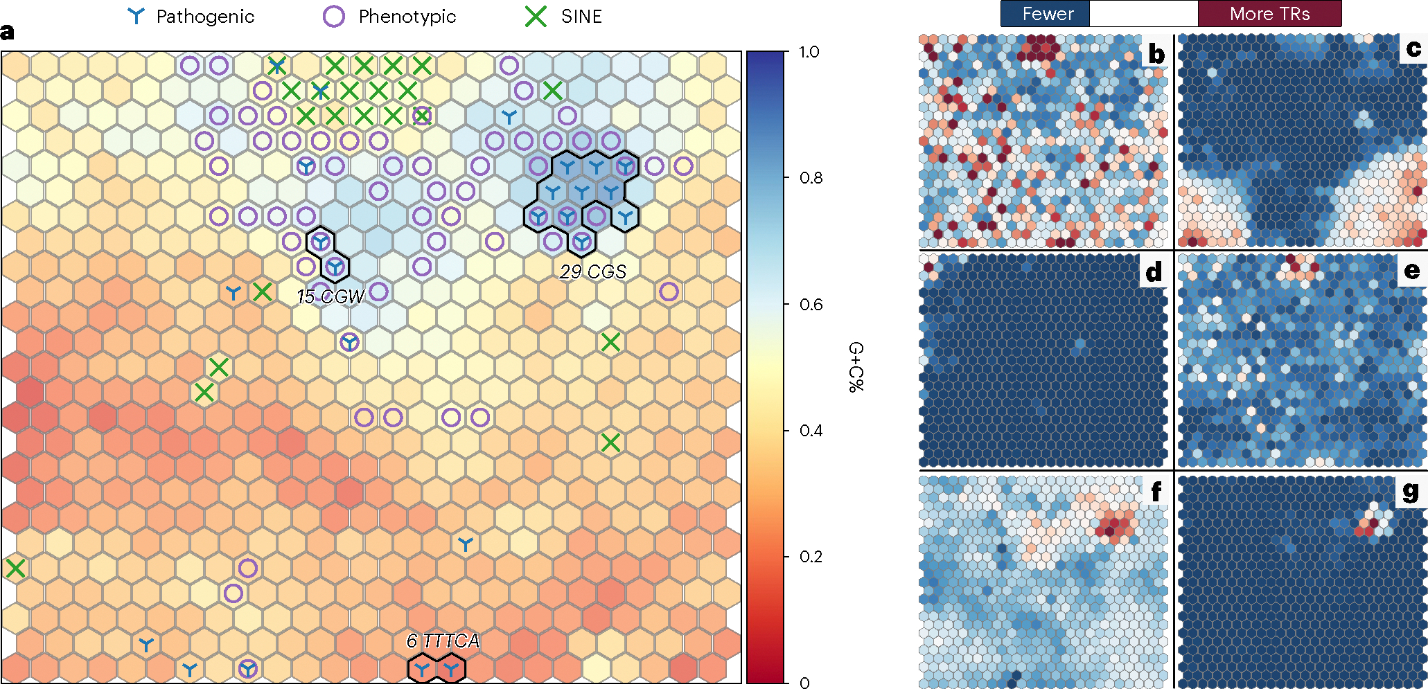
a, SOM using 4-mer frequencies per region with hue indicating mean G+C percentage. Dense known pathogenic neighborhoods are annotated with their most common motif using International Union of Pure and Applied Chemistry (IUPAC) codes (S = G|C, W = A|T). b, Number of TR regions per neuron. c, Average percentage of TR region sequence annotated as a homopolymer. d, Intersection of TR regions with UCSC microsatellite track exposes a neighborhood of microsatellites (top left). e, Visualization of UCSC segmental duplications track shows clustering in similar sequence contexts to SINEs in a (top middle). f, Map of TRs intersecting genes. g, Map of TRs overlapping promoters.

During the cataloging process, regions with only homopolymer annotations were removed. However, sequences with lower complexity may have been annotated as both a homopolymer run and, for example, a dinucleotide repeat. In these cases, the homopolymer annotation was removed and the dinucleotide annotation was preserved. To identify these ultralow-complexity sequences in the catalog, we recorded the percentage of a region’s sequence that was annotated as a homopolymer run. Figure 1c shows the mean percentage of the TR region sequence that was annotated as a homopolymer and exposes two dense concentrations in the bottom corners corresponding to sequence neighborhoods of ultralow complexity.

We further plotted TRs on the basis of their intersection with four reference annotation tracks to highlight their representation in our catalog. Microsatellites (Fig. 1d) formed a neighborhood in the top left, suggesting that they had a distinct sequence context. TRs overlapping segmental duplications (Fig. 1e) were mainly concentrated in the SINE neighborhood. TRs intersecting genes (Fig. 1f) and promoters (Fig. 1g) were highly concentrated in G+C-rich neighborhoods and, unsurprisingly, overlapped the bulk of known pathogenic TRs⁵⁴. These neighborhoods of TR sequence contexts overlapping various reference annotation tracks showcase the diversity and comprehensiveness of the TR catalog.

Polymorphism across TRs

Having defined a catalog of TR regions, we explored the variation within these regions across three independently derived HG002 assemblies, as well as 83 haplotype-resolved long-read assemblies of other individuals from multiple projects and populations^55–57 (Supplementary Table 4). This exploration helped us to understand the genetic diversity across each TR region while refining and annotating our benchmark. The assemblies were processed using Minimap2 (ref. 58) to produce alignments, paftools to call variants⁵⁸ and a custom pipeline to collect per-haplotype coverage of the assemblies. From these 86 assemblies, we created a unified set of variants as a project-level variant call format file (pVCF; see Methods for ‘pVCF generation’).

On average, haplotypes had a contig N50 of 35.3 Mbp. Assemblies produced by the Human Pangenome Reference Consortium (HPRC) (n = 46), which used hifiasm⁵⁹ to assemble PacBio HiFi reads with parental short reads, were found to be more continuous (mean haplotype contig N50 of 44.5 Mbp) than those produced by other projects (n = 39, N50 = 27.3 Mbp). Furthermore, the HPRC HG002 assembly underwent additional gap filling, scaffolding and curation to extend its continuity from an N50 of 86.3 Mbp to 121.2 Mbp (ref. 60). This set of 86 assemblies from 78 individuals produced alignments covering 96.7% of GRCh38 on average. We classified spans of the reference as being confidently covered by a sample if its haplotypes each produced a single alignment over a span. On average, assemblies produced by the HPRC confidently covered 96.2% of GRCh38 compared to 92.3% for the other projects (Supplementary Table 5). Therefore, we chose the HPRC HG002 assembly with super-scaffolding to produce the variant representations used by the TR benchmark.

Samples produced between 5.7 million and 10.2 million (mean: 7.2 million) confidently covered variants depending on their population (Supplementary Fig. 5). Despite the TR catalog covering only 8.1% of GRCh38, an average of 24.9% of variants per sample occurred within TR catalog regions. The observed enrichment of sample variation in TR regions increased with variant length, with an average of 21.2% of SNVs, 36.6% of indels that were less than 5 bp in length, 66.6% of variants that were between 5 and 50 bp in length and 72.2% of variants that were at least 50 bp in length occurring within TRs. Merging variants across samples produced a pVCF with a total of 124 million variants. We again saw a significant enrichment of variation in TRs (overlap permutation test, P < 0.001), with 20.7% of pVCF variants inside TR regions, and the same relationship between variant length and TR enrichment (Supplementary Table 6). Because variant counts can be sensitive to alignment parameters (that is, varying allelic representation), we also summed the length of all non-SNV variants in the pVCF and again found that 486 Mbp (41.0%) of the 1.1 Gbp of variant bases were within TR regions. These per-sample and pVCF variant metrics illustrate the highly polymorphic nature of TRs and their disproportionate contribution to genetic diversity.

This enrichment of variants was not uniformly distributed across TR regions. Of the 1.78 million TR regions in the catalog, 27.2% had no observed variation across the 86 assemblies, 47.4% had only small indels and 81.0% had no variant that was ≥5 bp in length. The 19.0% of the TR catalog with at least one variant that was ≥5 bp in length spanned 3.0% of GRCh38 and contained 70% of pVCF variants that were ≥5 bp in length. We attempted to replicate this observation by intersecting variants that were ≥5 bp in length from the SNP database (dbSNP version 153) across chromosome 1 (chr1) with the TR catalog and found that, while 79.1% of TRs had at least one dbSNP variant of any allele frequency (AF), 74.0% lacked a variant that was ≥5 bp in length with an AF of at least 1%. We then partitioned the regions on the basis of whether they contained a variant that was ≥5 bp in length in the pVCF and performed a permutation test on their intersection with protein-coding genes. This experiment showed that the 1,446,782 TR regions without pVCF variants that were ≥5 bp in length intersected genes as frequently as expected by chance (P = 0.45), while the 337,627 with variants that were ≥5 bp in length had significantly fewer intersections with genes than expected (P < 0.001). Thus, we observed a higher frequency of variants in TR regions compared to the rest of the genome, with larger variants being under-represented in protein-coding genes.

Formalizing the HG002 TR benchmark

To create an HG002-specific benchmark, we leveraged assemblies of HG002 from three projects. We then subset the TR catalog to regions that were confidently covered (once per haplotype) by the scaffolded HPRC HG002 assembly and an ‘alignment replicate’ of that same assembly created using different alignment parameters (see Methods for ‘Definition of benchmark regions and variants’). By analyzing two alignments of the same assembly with different parameters, we produced different sets of confidently covered TR regions and variant representations. Restricting the alignment to TR regions that were consistently covered by both the primary and the replicate alignment excluded regions that may have been overly subject to alignment ambiguities. Furthermore, a repeat region was excluded if either haplotype had a break in the assembly-to-reference alignment inside a segmental duplication, a TR longer than 10 kbp or a satellite repeat. We also excluded all gaps in the reference and homopolymers longer than 30 bp, because assembly-based variant calls are less accurate in these regions²⁷.

This curated set of confidently covered regions captured 1,706,853 TR regions (95.6% of the TR catalog) for inclusion in the benchmark across the autosomes and sex chromosomes (Fig. 2a). To assess the sequence composition of the benchmark’s TR regions, we again used the aforementioned kmer-based SOM, which clustered regions into neurons. An average (±s.d.) of 95.9% ± 3.8% of TR regions per neuron were captured in the benchmark (Fig. 2b and Supplementary Fig. 6). Some neurons (that is, collections of TR regions by sequence context) were captured below 90% because their TR regions were excluded from the benchmark during assembly curation. This was observed in the few highlighted (red) neighborhoods from Fig. 1c,e, which represent TRs by homopolymer sequence and intersection with segmental duplications, respectively, overlapping lowlighted (blue) neurons in Fig. 2b. The exclusion of long homopolymers from confidently covered regions caused a relative deficiency in the benchmark’s ability to assess TRs in sequence contexts with ultralow complexity. Nevertheless, 92.8% of TRs in neurons with ≥15% average homopolymer sequence across the region were still included in the benchmark (Supplementary Fig. 1). Therefore, TR regions with ultralow-complexity sequences were still represented. Similarly, 127,682 of 364,589 (35.0%) TR regions overlapping segmental duplications remained included in the benchmark.

Fig. 2 |. Location, sequence and length properties of the benchmark’s TR regions.

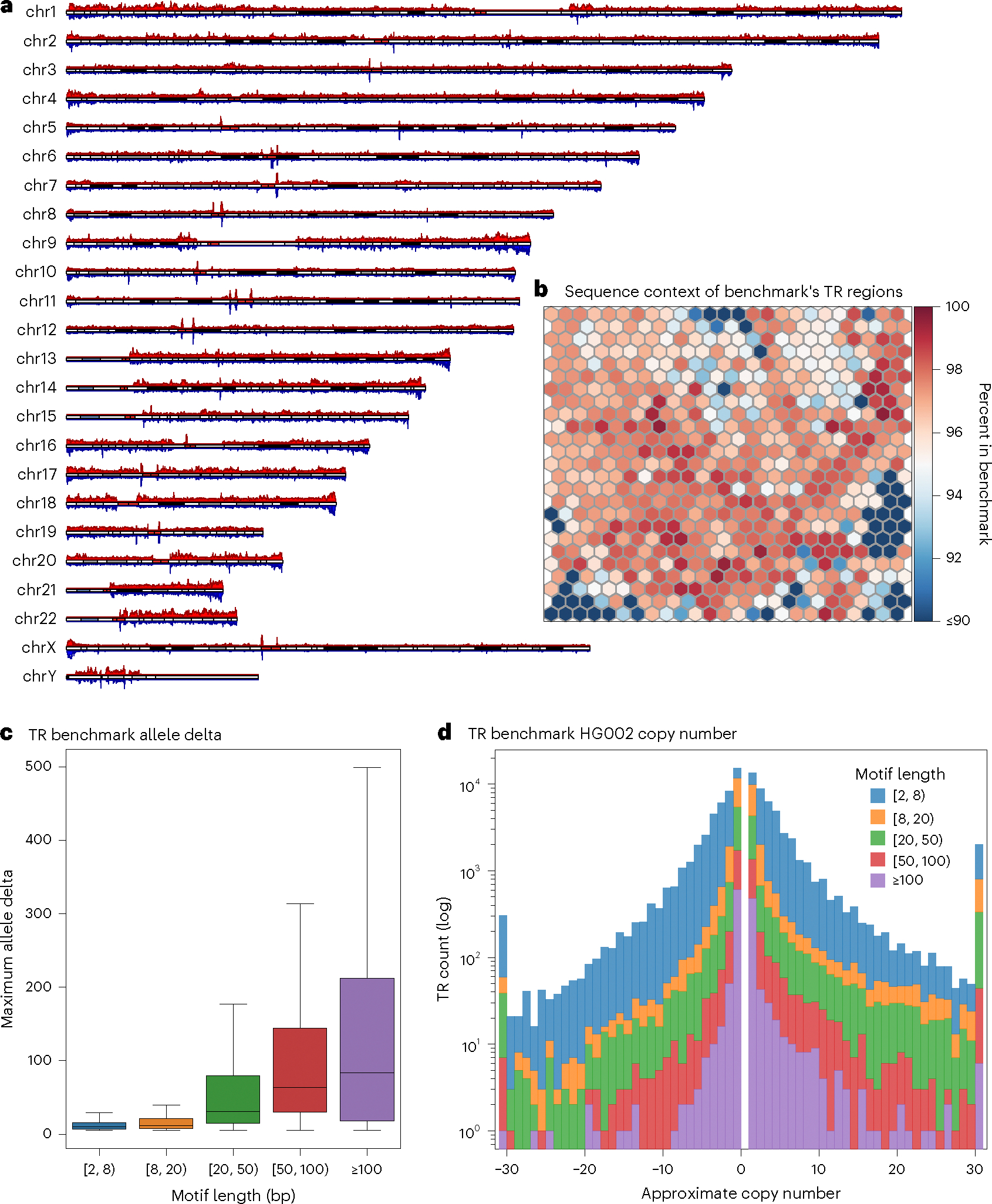
a, Karyoplot of TR regions. Top: TR regions included in the benchmark (red); bottom: catalog TR regions with HG002 variants that are ≥5 bp in length (blue). b, SOM heatmap representing the percentage of TR catalog regions per neuron contained in the benchmark with respect to Fig. 1b. c, Boxplot of HG002 allele deltas (sum of absolute variant lengths in base pairs) for 93,693 TR regions as a function of motif length (lower quartile, 25th percentile; upper quartile, 75th percentile; center, median; extrema, 1.5 times the interquartile range). In heterozygous regions, the maximum delta is used. d, TR allele delta length per region as a function of motif length. Contractions have a negative delta and expansions have a positive delta. Copy numbers greater than 30 are binned at either end of the histogram.

With the set of HG002 benchmark TR regions selected, we next characterized their variants and confirmed their validity using the HG002 replicate assemblies. We limited our investigation to variants that were ≥5 bp in length to avoid smaller base calling or consensus errors in assemblies. In total, 107,842 (6.3%) of the benchmark regions had variants in HG002 that were ≥5 bp in length and 346,935 (20.3%) had only SNVs and smaller indels, while 1,252,076 (73.3%) were reference homozygous (that is, they had no variants) and could, therefore, serve as negative controls during benchmarking. We next challenged the confidence of the benchmark’s variants that were ≥5 bp in length, as well as our ability to compare to these variants using techniques described below, thereby stratifying regions into confident (Tier1) and nonconfident (Tier2) sets accordingly. If the alignment replicate of the scaffolded HPRC HG002 assembly and at least one of the two technical replicates of HG002 in the pVCF confirmed the presence or absence of the benchmark’s ≥5-bp variation, the region was considered Tier1. The remaining regions were considered less confident and labeled Tier2, as they were more likely erroneous because of sequencing errors and/or errors in the assembler’s partitioning of haplotypes. In total, 96.0% (201-Mbp span) of the benchmark regions were classified as Tier1, leaving 4.0% (11.7 Mbp) as Tier2. Breaking this down further, a total of 1,616,956 (94.7%, 197-Mbp span) benchmark regions had unanimous agreement among the three assemblies (98.7% of Tier1 regions). The main source of TR regions being demoted to Tier2 status (63,671 of Tier2 regions; 93.1%) was a failure of both technical replicate assemblies to provide confident coverage over the region, which prevented the confirmation of HG002 haplotypes. A total of 845 benchmark regions had no agreement across the three replicates (1.2% of Tier2 regions). A full table with the counts of replicate states and their assignment to tiers is provided (Supplementary Table 7).

By definition, the set of TR catalog regions included in the benchmark was dependent on the location of TR regions. However, identifying the exact boundaries of TR sequences is difficult⁴⁰. Our TR catalog was also subject to these difficulties, as illustrated in the above analysis of the distribution of region buffer lengths. To ensure that the variation included in the benchmark was not overly subject to the region’s boundaries, we reprocessed the benchmark region selection and tiering processes after expanding the span of all TR catalog regions by 10 bp on both ends and compared the results to the unaltered benchmark. In doing so, we found that 180 extended benchmark regions were no longer confidently covered by the HG002 assembly, 389 regions were assigned different tiers and 2,968 had a variant that was ≥5 bp in length within the 10-bp extension. This suggests that only 0.2% of region boundaries in the benchmark could benefit from further refinement and, as a whole, the span of benchmark regions over variants was stable. Additionally, we found that 4,939 (3.4%) of variants that were ≥5 bp in length were within the buffer sequences of benchmark regions. These ‘buffer variants’ occurred in a total of 4,451 (0.2%) benchmark regions and were predominantly homopolymer runs (~40.4%).

Variant counts and sizes are often dependent on alignment parameters⁶¹, especially in TR regions. Therefore, it is useful to consider allele deltas, which are the sum of variant lengths per haplotype over a TR region. By comparing the maximum allele delta of HG002 haplotypes per region with the maximum TandemRepeatsFinder-annotated motif length collected during catalog creation, we saw a slight correlation of longer motifs creating larger allele deltas (Spearman correlation r = 0.33, P < 0.001; Fig. 2c). This pattern can be explained by the commonly accepted stepwise mutation model of TRs, which, among other things, describes expansions and contractions as occurring in whole repeat units (that is, motifs)². Furthermore, we could approximate the copy number change of TRs in HG002 by dividing the maximum allele delta by the longest annotated motif length (Fig. 2d). For example, a 10-bp allele delta over a TR region having a 5-bp motif comprises a two-copy expansion of the TR. We saw symmetry across the domain of approximate copy number changes with respect to expansions (positive allele deltas) and contractions (negative allele deltas). However, the range of TR counts showed slightly more expansions (52,658) than contractions (49,014). These analyses illustrate that the benchmark captures TR expansions and contractions of multiple copy numbers across motif lengths.

Next, we examined the completeness of the TR benchmark in complex or potentially consequential TR regions by analyzing the properties of TRs that intersect with 5,026 previously reported MRGs²⁹, known pathogenic TRs, VNTRs with reported phenotypic impacts and CODIS sites (Table 1). Of the nearly 300,000 TR regions in the catalog intersecting 4,866 of the MRGs, 96.8% were confidently covered by the assembly and included in the benchmark, with 92.8% being Tier1. Interestingly, 3,069 MRGs had at least one TR benchmark region with HG002 variants that were ≥5 bp in length, which is a subset of the 4,113 having variants that were ≥5 bp in length in the pVCF (median of seven pVCF variants per gene). For the 80.6% pathogenic, 98.2% phenotypic and 86.3% CODIS TRs included in the benchmark, 86.0%, 97.2% and 59.0% were labeled as Tier1, respectively. The pathogenic and CODIS subsets of TRs were generally more difficult to resolve and were classified as Tier2 because of both technical replicates failing to supply confident coverage for confirmation. In total, the technical replicate assemblies were unable to cover all 8 Tier2 pathogenic TRs, 17 of the 18 Tier2 CODIS TRs and 11,240 (95.7%) of the Tier2 TRs intersecting MRGs. Nevertheless, 64,386 of 66,465 (96.9%) benchmark regions intersecting pathogenic, CODIS or MRG TRs and containing HG002 variants that were ≥5 bp in length remained in Tier1.

Table 1 |.

Summary of TRs intersecting genomic loci

	n	Benchmark	Tier1	Tier2	HG002 ≥5 bp	Other ≥5 bp
MRGs	299,633	289,964	278,225	11,739	17,201	49,219
Pathogenic	62	50	43	7	25	42
Phenotypic	113	111	108	3	49	89
CODIS	51	44	26	18	25	44

MRGs constitute a collection of 5,026 previously reported genes across multiple clinical databases. A total of 4,866 (96.8%) MRGs intersected at least one TR. HG002 ≥5 bp denotes the count of TR regions with a variant that is ≥5 bp in length in the benchmark. Other ≥5 bp denotes the count of TR regions with a variant that is ≥5 bp in length in the pVCF from non-HG002 samples.

Enabling an accurate comparison of TR alleles

Having constructed the benchmark’s regions and variants, we next explored how to accurately perform a comparison to this collection of small and large variants because previous benchmarks separated variants by size. For this purpose, we first evaluated existing recommended methods for small variant comparison (RTG vcfeval⁶²) and SV comparison (Truvari bench³⁰) along with our newly developed variant comparison technique (Truvari refine). To assess the performance of comparison methods, we leveraged the same HG002 assembly but with different alignment parameters to obtain noticeably different allele representations for complex variants. This setup demonstrates the difficulties of TR variant comparison while allowing theoretically perfect precision and recall, because the TR benchmark regions contain only sites that were well covered by both alignments of the assembly and all discovered variants were derived from an identical input assembly.

In total, the TR benchmark produced 142,716 variants that were ≥5 bp in length (66,640 deletions and 76,076 insertions) and the alignment replicate produced 161,733 variants that were ≥5 bp in length (77,751 deletions and 83,982 insertions). When comparing the replicates with vcfeval or Truvari bench, we saw an F₁ score (that is, the harmonic mean of precision and recall) of 0.839 and 0.862, respectively. The unmatched variants remaining were caused by highly disparate variant representations and other allele size issues. To improve this, we designed Truvari refine, which achieved an F₁ score of 0.993. Comparison metrics are detailed in Supplementary Table 8. Analyzing the precision and recall of the benchmark’s alignment replicate by tier using Truvari refine showed 1.00/1.00 for Tier1 regions and 0.89/0.86 for Tier2 regions. The reported performance metrics for vcfeval and Truvari bench varied as a function of variant length for both Tier1 (Fig. 3a) and Tier2 (Fig. 3b) regions. On the other hand, Truvari refine’s Tier1 performance nearly reached a theoretically perfect precision and recall, while its Tier2 performance was less variable with consistently higher metrics than with the other approaches. The reported performance of vcfeval dropped off gradually after 20 bp in length and the tool could not compare variants that were >1 kbp in length by design. The vcfeval tool is also limited by the requirement that haplotypes match exactly, while Truvari’s core comparison approach can allow inexact matches, which is demonstrated by the better reported performance of Truvari bench, particularly after 200 bp. Of the 886 FNs and 1,088 FPs reported by Truvari refine, all but two FNs and six FPs were from Tier2 regions.

Fig. 3 |. Benchmarking pipeline performance.

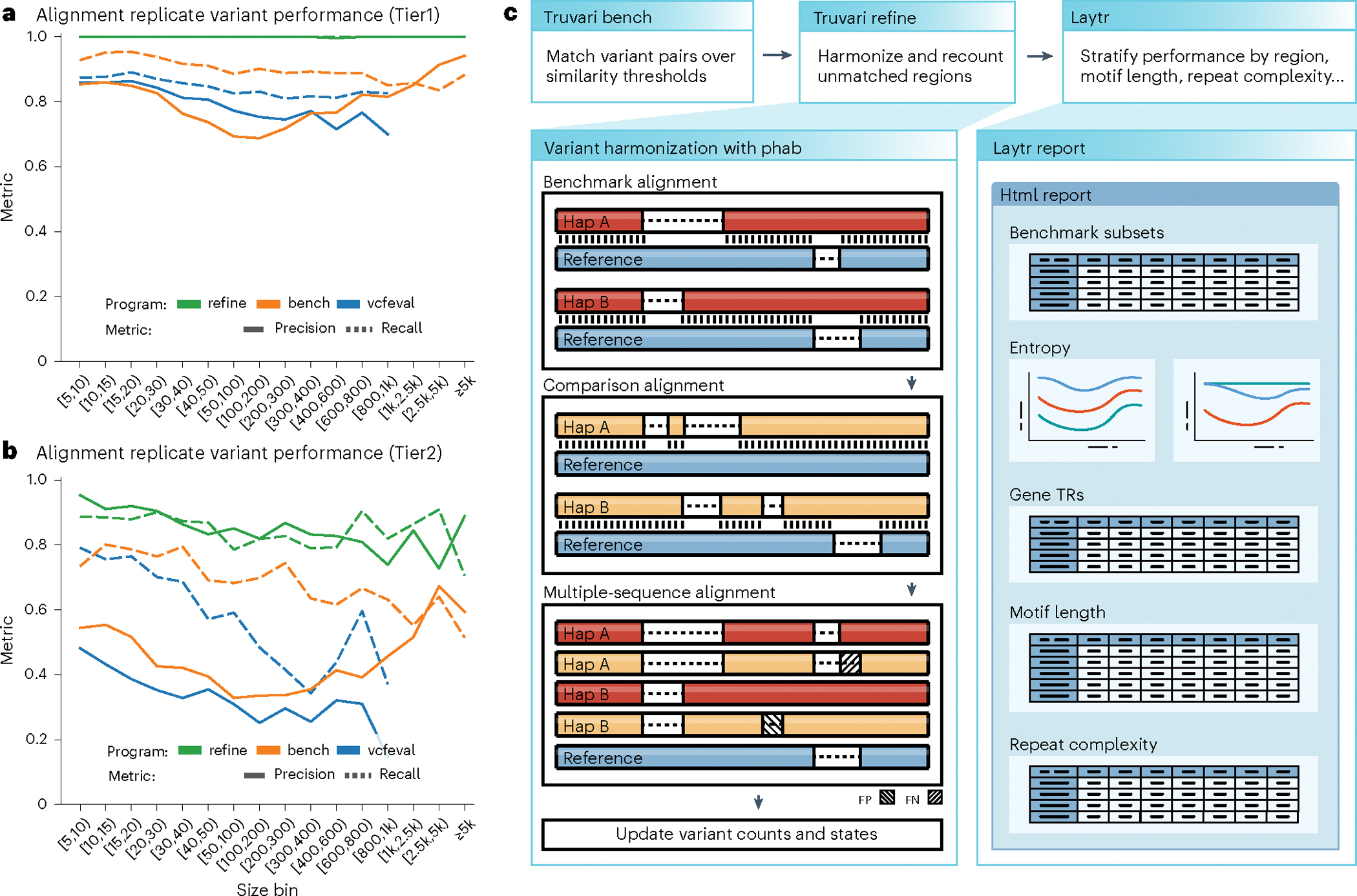
a,b, Size regime performance metrics for comparison tools (RTG vcfeval, Truvari bench and Truvari refine) on the HG002 TR benchmark against the alignment replicate for Tier1 (a) and Tier2 (b) regions. c, Pipeline schematic of Truvari operations for comparing sequence-resolved variants to the TR benchmark. Top: three commands for creating a benchmarking result and stratification report; left: illustration of Truvari phab variant harmonization; right: cartoon of Laytr stratification html report.

To accomplish the above-described improvements to variant comparison, we expanded the Truvari variant comparison tool’s pipeline. Details of the commands used by the workflow are available (Methods). Figure 3c (top) shows the principal steps of the comparison procedure. Briefly, to perform variant comparison of TRs, the Truvari bench subcommand’s result is used as input to the new refine subcommand. Refine first identifies benchmark regions with unmatched variants between the baseline and comparison VCFs. Variants in the identified regions are then harmonized with Truvari phab (another new Truvari subcommand) and recompared using Truvari’s core comparison approach. Summary metrics are then calculated using the original variant counts for nonharmonized regions and the harmonized comparison results for regions that were refined. The per-region summary can then be fed into Laytr (our benchmarking stratification tool) to generate more detailed reporting.

To accurately compare TRs for benchmarking, two main challenges needed to be addressed. The first challenge was that the benchmark has variants as short as 5 bp, which is smaller than Truvari’s previous minimum size of 50 bp. The second was that alignment and variant representation ambiguities can be enhanced in TR regions such that a one-to-one comparison is insufficient. Below, we detail the innovations now implemented in Truvari to overcome these challenges, as well as report simulation experiments that illustrate the impact of these changes on variant comparison.

Previously, variant comparison with Truvari used a ‘reference context’ approach to calculate sequence similarity, in which the alternate alleles of VCF entries being compared are each incorporated into the span of the reference covered by both variants¹⁰. This produces faux haplotypes, where differences in variant placement (for example, deleting the first copy versus the last copy of a TR) would have a lesser effect on sequence similarity. While this approach does overcome alignment ambiguities, the similarity scores are inflated by the shared reference context (that is, reference bases between two variants). This inflation becomes more problematic for smaller variants where reference bases in the sequence of faux haplotypes may outnumber those in the alternate sequence of variants. Hence, Truvari’s sequence comparison approach was modified to accommodate the possibility of TR expansions and contractions being placed at any position within the reference’s representation of the TR while removing reference bias. This is accomplished by ‘unrolling’ the alternate sequence of VCF entries in a manner akin to variant normalization’s left alignment⁶³. The difference is that left alignment preserves the order of nucleotides in alternate sequences, whereas unrolling does not. Instead, when unrolling a sequence from its current position to the position of the sequence to which it is being compared, for every base pair of the variant that is shifted upstream or downstream in another representation, the alternate allele’s base pair that is closest to the 3′ or 5′ end is moved to the beginning or end of the allele, respectively.

To test the accuracy of these sequence comparison techniques, we simulated ~12 million TR expansions with between 0% and 30% of bases randomly substituted in the expanded sequence to emulate sequence divergence. We then compared the simulated divergence to the reference context, unroll and direct comparison sequence similarities (see Supplementary Methods for ‘Simulation of TRs’). On average, the unroll sequence similarity differed from the simulated divergence by an average (±s.d.) of 0.07 ± 0.2 percentage points (pp), which was more accurate than the reference context similarity (4.3 ± 3.6 pp) and direct similarity (4.3 ± 5.5 pp). Supplementary Fig. 7 shows how the unroll sequence comparison was more tightly correlated (Pearson R = 0.99) to the simulated divergence than the reference context (0.67) and direct (0.61) similarity.

The second major improvement to Truvari’s comparison is a module for circumventing split variant representations. Split variants are seen when pipelines represent an identical haplotype with a differing number of variants (Fig. 3c, left). For example, a TR expansion can be represented as a single insertion with two additional copies of a motif or as two separate single-copy insertions of the motif. While each set of variants describes an identical haplotype, one-to-one variant comparisons report deflated similarity metrics as only part of the haplotype’s change in one representation is compared to the full change in the other. To address variant representation differences, a variant harmonization procedure (Truvari phab) was developed, which extracts sample haplotypes from VCFs before performing a multiple-sequence alignment (MSA) and recalling variants (Fig. 3c, left).

We simulated 30,000 TR expansions from the TR catalog without interspersed repeat annotations and with an average motif purity of at least 95% (see Supplementary Methods for ‘Simulation of TRs’). Each expansion was then given two variant representations by inserting the expansion at the beginning of the reference sequence and by inserting the expansion in at least two other positions. MSA harmonization reduced the average simulated number of variant positions per region from 4.11 to 1.87. Because performing an MSA is computationally burdensome, we also implemented an option to perform variant harmonization with the faster wavefront alignment (WFA)⁶⁴. While WFA is ~250 times faster than MSA, its independent pairwise realignment of haplotypes produces less parsimonious representations, with an average of 1.96 variant positions after harmonization.

The harmonization of variants alters their representations and their counts. This becomes a confounding factor for one’s ability to equate performance metrics between runs because the MSA performed causes the final count of baseline variants to depend on the joint alignment created with the comparison’s haplotypes. Therefore, we propose an alternative performance reporting scheme that measures per region instead of per variant (Supplementary Table 9). Furthermore, we designed the benchmark to also measure true negatives (TNs; that is, regions where no variant that is ≥5 bp in length should be observed). As discussed in previous sections, not every TR region has an HG002 expansion or contraction. Therefore, these reference-homozygous regions can be leveraged as negative controls in per-region performance metrics. Supplementary Table 10 demonstrates the per-region performance of the three HG002 replicates used for benchmark creation described above. The alignment replicate had a higher balanced accuracy of 0.996 compared to the two technical replicates with 0.990 and 0.989.

In addition to generating accurate comparisons to the TR benchmark, it is important that comparison results be informative. Throughout the creation of our TR catalog and the HG002 benchmark, as well as our analysis of comparisons to the benchmark, we collected many annotations (for example, the presence of interspersed repeats, the length and purity of constituent motifs, known pathogenic TRs and intersections with genes). To assist users in leveraging these annotations into informative stratifications, we also provide a new tool named Laytr. Laytr generates per-region performance metrics on ten standard stratifications of the benchmark (Fig. 3c, right). Laytr joins the Truvari refine region report to the catalog and benchmark data and processes the reported regions through the SOM. Laytr produces an html summary for visualization, as well as machine-readable files. As examples, Laytr reports from the long-read TR caller TRGT²⁰ and long-read whole-genome sequencing (WGS) SV caller Sniffles⁶⁵ are provided in Supplementary Materials 1 and 2. Comparing these two reports shows the added benefit of TR-specific callers, as TRGT has a balanced accuracy across Tier1 regions of 0.98 compared to Sniffles with 0.53. A considerable proportion of this difference is attributable to Sniffles reporting only SVs that are ≥50 bp in length, whereas TRGT genotypes across all allele lengths. This difference is detailed in the allele delta of the Laytr report, which stratifies performance by each region’s sum of variant lengths. This report shows that TRGT’s TP rate was consistently at ~0.98 across all size bins, whereas Sniffles began to find TPs from only 50 bp onward at an approximate TP rate of 0.62. Complete descriptions of Laytr stratifications and their interpretation are provided (Methods).

The Truvari refine and Laytr methods presented here enable precise variant comparisons, especially in TR regions, but their concepts can also be applied across other regions of the genome. Furthermore, they enable stratification and, thus, new insights into the performance of different technologies and methodologies to infer variants.

Insights into the use of the TR benchmark

To evaluate the benchmark’s use in exploring general patterns of TR discovery, we collected variant calls from seven tools that use different sequencing technologies and differing methodologies (Supplementary Table 11) and compared them to our benchmark. These analyses are not definitive assessments of any particular pipeline’s TR discovery capabilities; instead, they aim to ensure that the benchmark is capable of assisting pipeline evaluations. Four of the tools are TR-specific callers, which leverage a TR catalog to discover alleles. Two of the TR callers use long-read sequencing and two use short-read sequencing. The remaining three tools are designed for general WGS variant calling of different size regimes and discover TR alleles simply through their previously described prevalence.

As noted above, the number of variants reported after refinement is dependent on the comparison VCF. We found that, after harmonization, the benchmark’s 139,372 HG002 variants that were ≥5 bp in length became an average (±s.d.) of 150,508 ± 5,418 variants across the seven comparisons. However, using Truvari refine’s per-region summaries, we saw an average of 106,046 ± 1,191 baseline positive (having a variant) TR regions. The remaining variance in region counts was attributable to the MSA ‘resizing’ variants above or below the 5-bp minimum length threshold or shifting variants into or out of the TR benchmark’s regions. Nevertheless, the tighter standard deviation of per-region summaries allowed more consistent comparability across pipelines.

We next searched for patterns in the properties of TRs discovered across these tools stratified by the underlying read length. To do this, we first subset the benchmark to Tier1 regions with HG002 variants that were ≥5 bp in length that were analyzed across all tools (n = 60,325). We next marked TR regions where both short-read TR callers and long-read TR callers independently agreed in their benchmarking state (for example, TP and FP). By subsetting to TR regions analyzed by all TR callers and where two tools using the same category of read length agreed, we ostensibly limited the impact of the methods on performance to query for read-length effects. When comparing the states of regions with short-read caller agreement and long-read caller agreement (n = 40,546), we found that 27,807 (68.5%) regions were resolved as TP by both pairs of tools, 12,734 (31.4%) were resolved as TP by only the long-read tools and 5 were resolved as TP by only the short-read tools, although this will likely change as new tools are developed.

When searching for properties of TRs that could indicate whether they were resolved by only the long-read tools (long-read set, LRS) or by all TR callers irrespective of read length (all-read set, ARS), we found four annotations provided by the benchmark with a significant difference (Wilcoxon rank-sum P < 0.001). First, the average (±s.d.) maximum allele delta (total variant length) of a TP TR region in the LRS was 124 ± 471 bp compared to 11 ± 14 bp in the ARS. The TR region’s motif length was 43 ± 74 bp for the LRS compared to 6 ± 26 bp for the ARS. The average LRS region span was 593 ± 689 bp compared to 125 ± 150 bp for the ARS. We also found a lower LRS average motif purity (0.91 ± 2.5 for the LRS versus 0.95 ± 2.4 for the ARS). In summary, longer changes or motifs over larger TR regions, as well as sequence contexts with lower motif purity, were resolved more frequently by this set of long-read TR callers than the short-read TR callers used in the example.

In addition to the four TR callers, we leveraged three WGS callers and compared the TRs discovered by the two sets. Of the benchmark’s 101,704 Tier1 HG002 regions that were ≥5 bp in length, the TR callers had at least one TP state in 101,1080 (99.4%) regions, while 90,996 (89.4%) regions had a TP state from any WGS caller. A total of 90,812 (89.2%) regions were TPs in both sets, whereas 10,296 (10.1%) were found to be TPs exclusively by the TR callers and only 184 were exclusive to the WGS callers. Interestingly, both the long-read and the short-read TR callers contributed to the set of regions found exclusively by TR callers at 99.8% and 3.4% of regions, respectively. The increase in TRs resolved by TR callers highlights not only the value of focused TR discovery algorithms but also opportunities for WGS callers to extend the comprehensiveness of their reporting.

As noted above, these results will likely change as new callers are developed and optimized with this benchmark. In addition, the design of the current benchmark and tools does not permit fine-grained analysis of base-level sequence accuracy, which may be higher for short reads for TRs shorter than their read length. Therefore, going forward, this analysis should be interpreted as an example of the utility of the benchmark to evaluate several methods rather than an evaluation of how methods using short and long reads differ.

Diving into the benchmark and its advancements

Collecting alleles from multiple genetically diverse individuals allowed us to ensure that the HG002 alleles captured in the benchmark were representative of those found across individuals. When checking the 101,704 Tier1 benchmark regions with at least one HG002 variant that was ≥5 bp in length, we found that 99.7% had variants present in another sample that were ≥5 bp in length. However, 7.3% of these regions had non-reference HG002 haplotypes with less than 99% sequence similarity to haplotypes from all other samples and were, therefore, considered unique to HG002. Additionally, 181,006 (11%) Tier1 regions lacked an HG002 variant that was ≥5 bp in length but had such variants in another sample. The commonality of HG002 TR variation relative to other samples suggests that the performance of variant callers in discovering HG002 TRs may translate to comparable performance on non-HG002 samples, although it would be valuable to have TR benchmarks for diverse individuals in the future.

While this benchmark contains a comprehensive selection of TRs with respect to length and sequence composition, it is important to acknowledge the diversity of TRs that may arise at any given locus across individuals (Fig. 4). For example, when plotting the allele delta of four CODIS sites across 156 haplotypes from the 78 unique samples in the pVCF (Fig. 4a), we observed contractions up to 60 bp in length and expansions as large as 100 bp. Focusing on just the CODIS PentaE site (Fig. 4c) and plotting the unique-by-length haplotypes with TRviz⁶⁶, we saw HG002 AFs of 0.09 and 0.02 for the paternal and maternal alleles, respectively. These HG002 alleles (10 and 18 copies of the 5-bp repeat) were less common than the eight-copy allele with an AF of 0.13. The distinction between resolving a locus for a single individual versus all possible allele lengths is especially pertinent to pathogenic repeats (Fig. 4b). HG002 represents a healthy individual; thus, repeat expansions that are implicated in disease phenotypes are not represented. In Fig. 4d, a wide range of copy numbers can be seen across the JPH3 (ref. 67) locus, but all samples were below the pathogenic length of ≥41 copies. However, in Fig. 4e, two haplotypes can be observed above the pathogenic length of ≥50 copies for TCF4 (ref. 68). These TCF4 expansions were up to ~90 copies of the trinucleotide repeat, whereas HG002’s longer paternal allele was only ~30 copies. Therefore, researchers with an interest in TCF4 would need to account for a pipeline’s ability to resolve the locus in the benchmark, as well as the pipeline’s ability to resolve other HG002 loci with longer expansions.

Fig. 4 |. Diversity of TRs over 156 haplotypes at CODIS and known pathogenic loci.

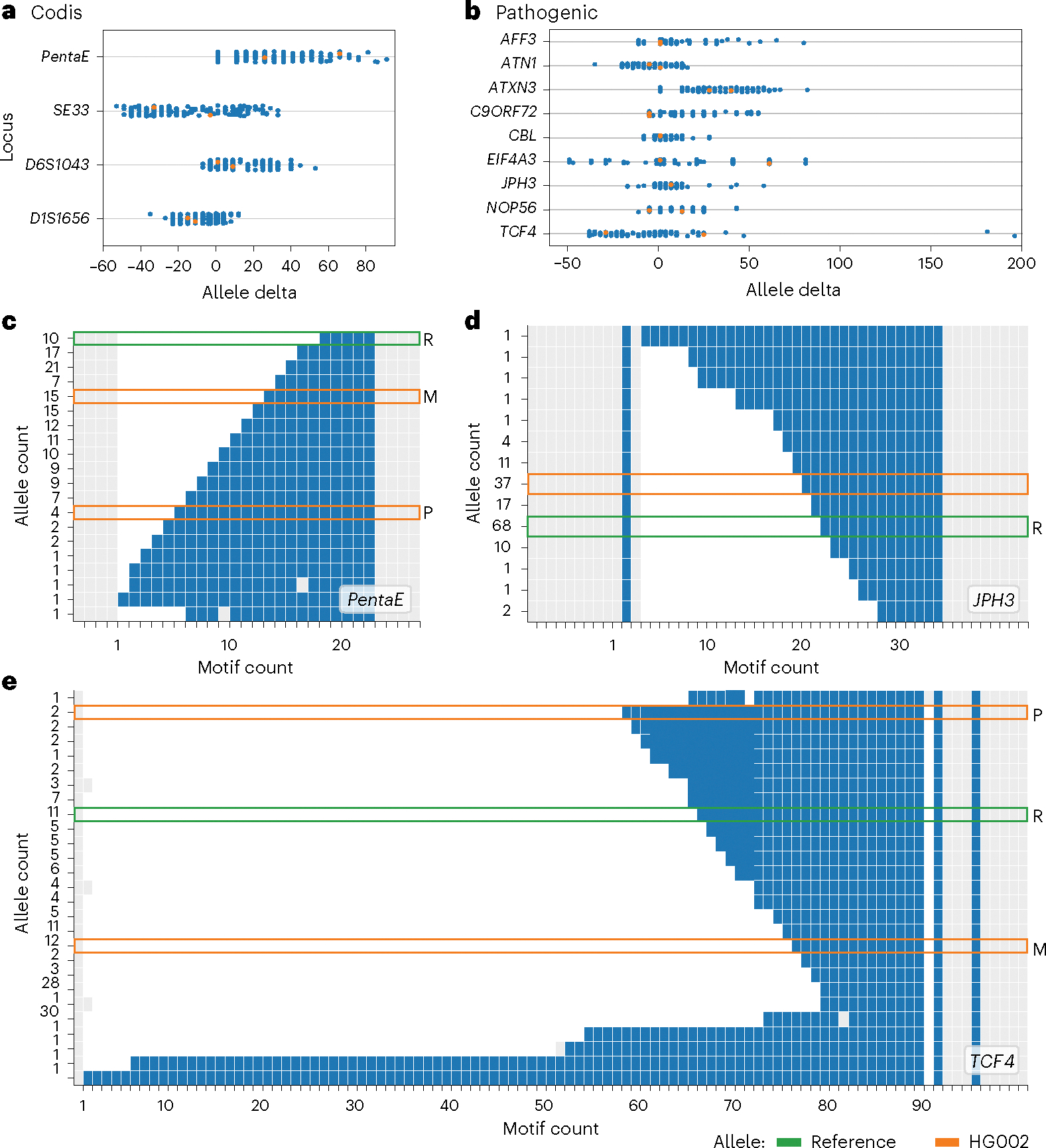
a, Allele delta (sum of variant lengths) across four CODIS loci. HG002’s maternal and paternal alleles are indicated by orange data points. b, Allele delta of nine known pathogenic repeats. c–e, Distribution of haplotypes over CODIS PentaE locus (c) and known pathogenic JPH3 (d) and TCF4 (e) loci. For c–e, each row represents a unique-by-length haplotype (allele) and the y label represents the number of haplotypes with the allele. Blue squares indicate the TR motifs, gray squares indicate the non-motif sequences and white squares are gaps introduced by MSA. Gray squares upstream and downstream of the TR are the buffer sequences of the benchmark’s TR regions. Orange boxes indicate HG002’s maternal (M) and paternal (P) haplotypes (homozygous regions have one box) and green boxes indicate the GRCh38 reference allele (R). The allele count was determined by deduplicating haplotypes by length.

Given that this TR benchmark is preceded by multiple GIAB benchmarks, we next investigated the intersection of the TR benchmark with previous GIAB benchmarks to understand what variants and segments of the reference are newly covered (Supplementary Table 12). Both the GIAB version 0.6 SV benchmark²⁸ (lifted over from GRCh37 to GRCh38) and the GIAB version 4.2.1 small variant benchmark²⁷ showed large overlaps with the TR benchmark of 95.1% and 84.5%, respectively. However, they were constrained in the variants that they reported in these regions. This is highlighted by the fact that the TR benchmark included 126,909 small (5–50 bp) and 18,720 large (≥50 bp) variants, which was much higher than in previous benchmarks (for example, the version 4.2.1 small variant benchmark with 89,029 small and 204 large variants). Thus, the benchmark’s Tier1 regions include variants that were otherwise not captured in existing benchmarks and present opportunities for the community to improve variant-calling methods.

To further gain insights into the validity of these variants, we collected seven variant callsets across multiple sequencing technologies and analysis techniques (SNV, SV and TR calling methods; Supplementary Table 11). We investigated whether TR regions in the benchmark where Truvari refine did not assign a TP or TN state to any caller’s result could be a signal that the benchmark’s variants may be incorrect. In total, we found 875 (0.05%) TR regions in which all callers disagreed with the benchmark. Of these benchmark regions, 866 were also found to be contradicted by the comparison to the high-quality GIAB version 4.2.1 small variant benchmark²⁷. Therefore, these regions likely did not hold accurate descriptions of HG002 TR variants and should be deprioritized for benchmarking. Fortunately, 473 (54.0%) of these suspect regions were already demoted to Tier2 status by the quality control techniques used during creation of the benchmark and the 402 remaining regions were demoted to Tier2 status in the final published benchmark.

To further ensure the reliability of the benchmark’s ability to identify errors, we manually curated a random selection of Tier1 TR regions with common FP and FN results from callers. We sampled 20 of the 866 (0.05%) Tier1 TR regions where only one comparison callset matched the benchmark. We found that eight appeared clearly correct in the benchmark and the comparison callsets were inaccurate because of long homopolymers or mapping issues stemming from a gene conversion-like event and a false duplication in GRCh38. Another four were in TR regions that spanned longer than the length of short reads and where long reads were noisy; however, the benchmark appeared to be correct or within one TR unit of the correct size but the exact length of the variant was unclear because of noise in the long reads. For another three, the benchmark was off by 1 or 2 bp in homopolymers or dinucleotide repeats. The remaining five were incorrect in the benchmark because of the super-scaffolded HPRC assembly having collapsed haplotypes caused by the assembler failing to separate the heterozygous events in an otherwise highly homozygous region, as previously observed²⁷. Because the benchmark was correct or close to correct even for these variants where most callers disagreed, we kept this as version 1.0 of the benchmark without further refinement.

Discussion

Here, we established a TR benchmark to promote the detection and inclusion of variants across TRs in research and clinical settings. This was accomplished by consolidating multiple TR annotation sources and producing a TR catalog of 1.7 million regions spanning the human genome. On the basis of 86 haplotype-resolved assemblies, including three HG002 assembly replicates, we were able to form a variant catalog of events that were ≥5 bp in length, which branches across the traditional variant size categories. Despite only ~8.1% of GRCh38 being covered by the TR catalog, its regions include a disproportionate number of variants (24.9% of variants per sample). In fact, 66.6% of variants with a length between 5 and 50 bp (that is, indels) and 72.2% of variants with a length of at least 50 bp (that is, SVs) occur within TRs, implicating an outsized contribution of TRs to genetic diversity and the importance of comprehensive TR characterization for genomic studies.

Many TRs were excluded in previous GIAB benchmarks because of the technical problems associated with both characterization and benchmarking caused by TRs²⁵. However, in this study, we addressed many of these prohibitive issues and included new spans of the reference. This TR benchmark across allele sizes and sequence contexts required an extension of Truvari’s variant comparison capabilities, including an improved sequence comparison technique and variant harmonization procedure to reduce representational ambiguities among callsets. These advances in comparison methodology also required the development of an approach to collecting performance metrics in the aforementioned per-region counting metrics. While counting by variants is still useful, assigning states to entire regions was shown to allow a more consistent comparison of benchmarking results.

We also introduce TN regions, which are TRs where HG002 contains a reference allele. This is particularly interesting because the complexity of TRs can lead to sequencing errors, misalignments or other sources of noise, which variant identification methods need to handle. Thus, the simultaneous assessment of TP, TN, FP and FN forms a comprehensive assessment of variant identification methods across the next frontier of genomics and likely clinical genomics as more diseases are linked to TR mutations.

We further provide multiple annotations over the TR catalog and benchmark regions, as well as the new tool Laytr, to facilitate stratification of results. We highlight the contribution of specialized TR callers through analysis of multiple TR and variant discovery methods. Furthermore, we report general patterns of the contribution of TR callers when averaged within the read length they leverage. By subsetting the catalog to regions analyzed by all tools and with agreement across callers, we limited the analysis to a very conservative set of regions. Fully investigating a pipeline’s capabilities would require a more fine-grained analysis that is best directed by its maintainers. Therefore, we caution against the overinterpretation of these results as they are not representative of any particular pipeline’s limitations. Instead, our aim in these experiments was only to exemplify the use of the benchmark in hopes that developers of TR discovery pipelines may fully explore the relative strengths and weaknesses of their technologies.

We incorporated information on known pathogenic and phenotypic TRs into our TR catalog, together with CODIS TRs that are often used for forensic identification. Nevertheless, some of the most complex TRs were excluded because of a lack of confirmation from the replicate assemblies and were classified as Tier2. This includes, for example, 18 Tier2 CODIS regions across autosomes and sex chromosomes. Tier2 regions are considered less reliable for comparison and calculation of performance metrics but still likely harbor interesting variation that should be further investigated and improved upon.

As the HG002 cell line represents only a single individual, we investigated the allelic diversity across multiple samples to ensure that the TRs were typical of what is expected across a diverse set of individuals. Overall, 99.7% of the regions that carried a mutation in HG002 also carried a non-reference allele across the other 83 assemblies assessed. However, it is important to note that HG002 represents a healthy individual and repeat expansions associated with disease phenotypes are not represented. As shown in Fig. 4, HG002 represents the human population diversity well across different pathogenic variants. Because TRs are so diverse, we provide the pVCF containing 86 samples with 78 unique individuals for researchers to compare against. While only HG002 was curated, the other samples may be of assistance as controls.

Our work here focused on TR regions defined by the reference; however, TRs also formed at loci not initially represented in the reference genome. Future work could explore these cases to benchmark the ability of methods to identify novel TR regions. Additionally, mosaic variants often occur at low frequency within a sample and are likely enriched in TR regions, as they might form the basis of the observed diversity. Given our focus on the reliability of our Tier1 regions, we used assemblies to compile variants. Thus, low-frequency mutations are not reported as they are not produced by diploid assemblies. Characterizing mosaic variants in the individual or cell line will require a deeper interrogation of the error modalities of each technology in TRs, as it can be hard to distinguish sequencing errors from mosaic variants and errors in repeats can be correlated across technologies.

Overall, the methodologies developed here for the comparison of variants across TRs will push genomic and genetic research forward. We hope that this work can provide great assistance to other studies aimed at generating comprehensive whole-genome analysis that spans variant sizes and locations.

Online content

Any methods, additional references, Nature Portfolio reporting summaries, source data, extended data, supplementary information, acknowledgements, peer review information; details of author contributions and competing interests; and statements of data and code availability are available at https://doi.org/10.1038/s41587-024-02225-z.

Methods

Parameters for the software used in analysis are presented in Supplementary Table 13.

Definition of TR catalog

TR bed files from nine sources were collected^{6,17,20,36,54,69–71} (Supplementary Table 1). Intervals were filtered to exclude spans smaller than 10 bp or greater than 50 kbp in length before performing intrasource merging and boundary expansion of ±25 bp using bedtools (version 2.31)⁷². Intersource merging was then performed, again using bedtools, merging intervals with ≥1 bp of overlap. This procedure resulted in 2,171,789 candidate TR regions spanning 10.5% (308 Mbp) of GRCh38. The sequence spanned by each candidate interval was then analyzed by TandemRepeatsFinder³⁸ to capture TR motifs and reference copy numbers. Each interval’s annotations were then processed to create the final simplified TR catalog. A custom script then pulled reference sequences spanned by intervals and processed them with TandemRepeatsFinder (version 4.09.1)³⁸ and RepeatMasker (version 4.1.4)³⁹. TandemRepeatsFinder was run with a minimum alignment score threshold of 5, which is much lower than the recommended default of 50 that was used to create the University of California, Santa Cruz (UCSC) SimpleRepeats track. This lower score allowed more sensitive discovery of TR annotations over the intervals. RepeatMasker hits with scores of at least 225 were recorded. TandemRepeatsFinder annotations were grouped per region and redundancies were removed using a custom simplification script. The simplification script removed annotations of homopolymer motifs and annotations that overlapped a longer spanning annotation unless one of the following conditions was met: (1) the boundaries of the shorter annotation were entirely within the span of a single motif from the longer spanning annotation and (2) the shorter annotation boundaries were directly adjacent to a single motif copy of the longer spanning annotation. These two conditions preserved annotations with a parent or nested repeat structure and annotations with an unclear start or end between plausibly adjacent repeats, respectively. TR regions without TandemRepeatsFinder annotations after simplification were removed. Information about each region’s number of annotations, the overlapping relationship of annotations, the percentage of span annotated, the RepeatMasker highest-scoring hit class, intersection with Ensembl (version 105)⁷³, intersection with CODIS⁴⁴ and known pathogenic repeats was recorded before uploading the catalog to Zenodo⁷⁴. Full descriptions of the catalog’s columns and definitions can be found in Supplementary Table 2.

Collection of and motif comparison to known pathogenic repeats and phenotypic VNTRs

Known pathogenic TRs were collected from STRipy³⁵, gnomAD⁴⁵ and studies by Stevanovski et al.⁴⁶, Dolzhenko et al.¹⁷, Pellerin et al.⁴⁷ and Tan et al.⁴⁸. TRs were then consolidated by gene name and overlap of their genomic coordinates was manually ensured. Genomic coordinates per TR were then selected by preference in the order STRipy, gnomAD, Stevanoski, Dolzhenko, Pellern and Tan. This consolidation resulted in 68 total loci. Additionally, 118 VNTR-length protein-coding repeat polymorphisms were collected from Mukamel et al.⁴⁹. The final consolidated set of 186 TR loci is available in Supplementary Table 14. To compare motifs between the reported known pathogenic and phenotypic repeats and the TR catalog, sets of forward and reverse complement sequences from these motifs were generated and intersected. If any motifs were present in the intersection, the site was considered matched and, as such, accurately annotated. Furthermore, we allowed ‘Ns’ in the reported motifs to match to any base. Finally, we performed manual inspection of the known pathogenic repeats and found that four additional TR regions in the catalog did not match the above criteria because of a nonparsimonious representation of the reported motifs; for example, TMEM185A’s reported CCG motif is equivalent to the catalog’s CCGCCG and ZIC2’s GCN motifs match GCAGCGGCG.

pVCF generation

Haplotype-resolved long-read assemblies from three sources^55–57 were collected (Supplementary Table 4). The HPRC HG002 assembly that was further processed to increase continuity⁶⁰ was used in place of the original HPRC HG002 assembly. Each haplotype was aligned using Minimap (version 2.24)⁵⁸ and variants were called using paftools, which is packaged with Minimap. Custom scripts were used to generate per-haplotype coverage bed files. BCFtools (version 1.12)⁷⁵ was used along with custom scripts to perform intrasample merging and intersample merging. Finally, allele depth information was added to the pVCF using the aforementioned coverage bed files. Coverage bed files per haplotype per sample were intersected to identify confidently covered regions of the genome covered by exactly one alignment per haplotype for the autosome. The chrX confident regions were also defined as one alignment per haplotype for female samples and this was also applied to pseudoautosomal regions of chrX for male samples. The chrY confident regions were not collected for female samples and the nonpseudoautosomal regions of chrX for male samples were checked for one alignment across haplotypes. The 86-sample pVCF called against GRCh38 is available on Zenodo⁷⁶. The GRCh38 version used did not include alternate loci or decoy sequences (https://ftp-trace.ncbi.nlm.nih.gov/ReferenceSamples/giab/release/references/GRCh38/GCA_000001405.15_GRCh38_no_alt_analysis_set.fasta.gz). Enrichment of variation was tested with regioners (see Results for ‘Polymorphism across TRs’) using the pVCF reformatted to bed format and the TR catalog (version 1.1) with shuffle randomization. Intersection of TR regions with protein-coding genes was performed by separating TR regions with at least one variant that was ≥5 bp in length from TR regions without any variations. Each set was then intersected to Ensembl (version 105)⁷³ protein-coding gene transcripts with regioners using per-chromosome circular randomization.

Definition of benchmark regions and variants

The HPRC HG002 alignment coverage bed files built as described above (see Methods for ‘pVCF generation’) were subset to spans of the reference covered by a single contig per haplotype using custom scripts. This script only includes regions singly covered by each haplotype (that is, diploid coverage) for autosomes and single coverage for sex chromosomes with the exception of the chrX pseudoautosomal regions, as provided by dipcall⁷⁷, which were subset to spans covered singly by each haplotype. Furthermore, a second alignment of the HPRC HG002 assembly was performed using dipcall and custom Minimap2 alignment parameters designed to align across complex variants and larger SVs, originally used for the major histocompatibility complex region⁷⁸ (Supplementary Table 13). This produced a second VCF, as well as a bed file of regions covered once per haplotype assembly, with the same exceptions for the sex chromosomes as described above. The dipcall bed file was then curated to exclude reference regions and genomic alignments known to be problematic for benchmark generation. This included portions of alignments with a break in the assembly-to-reference alignment inside a segmental duplication, a TR longer than 10 kbp or a satellite repeat. We also excluded all gaps and homopolymers longer than 30 bp because assembly-based variant calls are less accurate in these regions. Both high-confidence bed files were then intersected to produce a final set of genomic regions representing those confidently covered by both alignments of the super-scaffolded HPRC HG002 assembly. The TR catalog was then subset to TR regions contained entirely within the boundaries of a confidently covered region. All bed file operations were performed using BEDtools (version 2.30.0)⁷².

The super-scaffolded HPRC HG002 assembly was then compared using Truvari (version 4.1) to each alignment replicate, as well as the Garg and Ebert HG002 technical replicates. To compare the benchmark to the technical replicates, Truvari refine was run with each sample’s bed file of confidently covered regions. The Truvari refine per-region bed files, which contained the coordinates and evaluation states of the initial benchmark regions (that is, TP, TN, FN or FP) were then joined across the comparison to the alignment and each technical replicate. Regions with a TP or TN state from comparison to the alignment replicate, as well as at least one of the technical replicates, were classified as Tier1 and those failing this condition were classified as Tier2. Furthermore, sites where the state flipped between replicates (for example, TP in the alignment replicate but TN in a technical replicate) were assumed to be unreliably compared and, therefore, demoted to Tier2. The union of states for the three replicates was also recorded as an annotation column in the benchmark bed (for example, TP_FN_FP corresponds to a TP in the alignment replicate, FN in the Ebert technical replicate and FP in the Garg technical replicate).

More annotations were then added to the benchmarking regions. First, the variants from the pVCF were analyzed for each benchmarking region to populate a ‘variant flag’. This flag uses bit encoding to indicate whether HG002 has a variant that is ≥5 bp in length (bit 0×1), HG002 has a variant that is <5 bp in length (0×2), another non-HG002 sample in the pVCF has a variant that is ≥5 bp in length (bit 0×4) or a non-HG002 sample in the pVCF has a variant that is <5 bp in length (bit 0×8). Additionally, when analyzing the pVCF, we summed the length of non-SNV variants for the maternal and paternal haplotypes in HG002 to record the region’s allele deltas. For example, a heterozygous 5-bp deletion on the maternal allele and a second homozygous 5-bp deletion would create a maternal allele delta of 10 bp and a paternal allele delta of 5 bp. Finally, the Shannon entropy of the sequence spanned by the benchmarking region was calculated⁷⁹ for the identification of low-complexity sequences.

Lastly, an additional copy of the VCF containing HG002 variants is available with ‘INFO’ fields of TandemRepeatsFinder annotations on reference sequences after incorporating a variant into the TR regions. This was created using Truvari anno trf, which populates INFO fields as follows: TRF, entry overlaps a TR region; TRFdiff, entry’s TR copy is different from reference annotation; TRFrepeat, repeat motif reported by TandemRepeatsFinder; TRFovl, percentage of variant covered by TandemRepeatsFinder annotation; TRFstart, start position of annotated repeat; TRFend, end position of annotated repeat; TRFperiod, period size of the repeat; TRFcopies, number of motif copies aligned with the consensus pattern; TRFscore, alignment score; TRFentropy, entropy measure; TRFsim, similarity of variant sequence to generated motif faux sequence.

Description of benchmarking software

Benchmarking results created using RTG vcfeval (https://github.com/RealTimeGenomics/rtg-tools) used version 3.12.1. Benchmarking results created using Truvari³⁰ used version 4.1. While Truvari’s core variant comparison approach was previously published, for this project, three additional features were developed to address the challenges of comparing variants with a length between 5 bp and 50 bp, harmonizing variant representations and generating performance reports for harmonized variants and the TR regions.

To handle the comparison of variants as small as 5 bp in length, the previously described³⁰ reference context sequence similarity approach was replaced with an unroll sequence similarity technique. The unroll technique works by first extracting the deleted reference sequence or inserted alternate sequence from two variants (denoted varA and varB). Next, the difference in start positions (posDiff) is calculated by subtracting varB’s start position from varA’s start position. If posDiff is negative, varA and varB are swapped and the absolute value of posDiff is taken. The number of base pairs that need to be unrolled from varB (urLen) is calculated as the posDiff modulo the length of varB. The last urLen base pairs of varB’s sequence are then swapped with its sequence up to urLen. This is effectively equivalent to iteratively moving varB upstream by posDiff base pairs and swapping varB’s base pair closest to the 3′ end to the 5′ position of the sequence for each base moved. For example, imagine a reference sequence of ‘ATC’. We could have an expansion of this motif represented by an insertion at the zeroth position with an alternate sequence of ‘ATC’ or an insertion at the second position of ‘CAT’; both of these variants would create a haplotype of ATCATC. The posDiff of these two variants is 2 and the urLen is 2 % 3 = 2, thereby moving the second variant’s last two bases (‘AT’) to the beginning, which creates ‘ATC’. The edit distance is measured using edlib⁸⁰ and is then converted into the longest common subsequence normalized sequence similarity using the following formula: 1 − edit_distance(varA, varB)/(len(varA) + len(varB)).

Variant harmonization was performed with a new Truvari command named ‘phab’. Inputs to phab include a VCF with phased variants, the reference against which the variants were called and a set of regions to be harmonized. Using pysam, a Python wrapper of htslib⁸¹, consensus sequences for haplotype 1 and haplotype 2 were created for each region. Each region’s haplotypes and reference sequence were then sent to MAFFT⁸² to perform MSA. MAFFT parameters were automatically chosen using their available auto option. Alternatively, haplotypes could be independently aligned to their reference sequence with pyWFA, a cpython wrapper of WFA⁶⁴ for harmonization (https://github.com/kcleal/pywfa). Truvari then converted the resultant MAFFT MSA or pyWFA pairwise alignment CIGAR strings back to VCF format.

Because some TR regions may not benefit from variant harmonization (for example, some regions may have no variants from the benchmark or comparison callset), it was unnecessary to run phab on all regions. We automated the selection of TR regions that could benefit from variant harmonization using another new Truvari command named ‘refine’. As input, refine takes a reference and a result from Truvari bench, which is a directory containing VCFs for the TP baseline, TP comparison, FN variants and FP variants, as well as summary statistics and parameters provided to the call to Truvari bench. For each benchmarking region, the VCFs are parsed and variants are counted. Each region with at least one FP variant and one FN variant (which can benefit from variant harmonization) is collected and sent to phab. Refine then recompares the phab output VCF holding the harmonized variants of the baseline and comparison samples using the Truvari bench parameters initially provided by the user. For some benchmarking experiments, it may be beneficial to recreate haplotypes over all variants in the baseline and comparison VCFs (specifically SNVs and indels smaller than 5 bp in length) instead of just the filtered set of variants contained in the initial Truvari bench output. Truvari refine provides a ‘use-original-vcfs’ parameter, which will automatically pull variants from the original VCF files instead of the consolidation of benchmark result VCFs. One may want to use the original VCFs when recreating haplotypes where small variants would make more accurate haplotypes and would improve harmonization. Finally, the phab harmonization’s bench result is consolidated with the variant counts from regions that were not refined to create the final performance metric summary.

Because the Truvari phab variant harmonization process may alter variant counts, we also added a new element to the Truvari refine output, which writes each benchmarking bed region with additional columns containing TP, FN, etc. variant counts before and after Truvari phab was run. Each region is then assigned a TP state if all variants in the region are matched between the baseline and comparison VCFs. If there are no variants in the region from either the baseline or the comparison VCFs, the region is assigned a state of TN. If there are any unmatched variants from the baseline and/or comparison VCFs, the region is assigned a state of FN and/or FP, respectively. These region state counts are then summarized and the per-region metrics are calculated. The set of per-region metrics and their definitions are provided in Supplementary Table 10.

Some TR callers may leverage a catalog of reference TRs that do not exactly match the loci provided in this work’s TR catalog. To facilitate benchmarking of these loci, Truvari refine has a ‘regions’ parameter, which a user can provide to subset the set of benchmark regions provided to Truvari bench using the ‘includebed’ flag. This procedure causes Truvari refine to calculate performance metrics over only the set of benchmark TR regions that were analyzed by the TR caller. Furthermore, if a user wishes to use the coordinates of a TR caller’s catalog instead of the TR benchmark’s regions, the user may provide the ‘use-region-coords’ flag to Truvari refine. Basic recommended default parameters for Truvari benchmarking of TRs are available in the README file that accompanies the benchmark files. Documentation on all of Truvari’s commands and their parameters is available from the GitHub repository’s wiki (https://github.com/ACEnglish/truvari/wiki).

To facilitate stratification analysis of Truvari results, we created a separate tool named Laytr (https://github.com/ACEnglish/laytr). Laytr joins the above-described per-region report with the original TR benchmark bed file and the full TR catalog. This master table of region states and all available annotations described above is then grouped by various columns in the table and the per-region metrics are recalculated. Additionally, Laytr takes the SOM that was built for this publication, which is distributed with the benchmark as input, and builds hexagonal heatmaps similar to those found in Fig. 1 with the balanced accuracy per neuron, accuracy per neuron and F₁ score per neuron. The analyzed and reported stratifications are classified into nine sections: benchmark subsets, entropy, gene TRs, interspersed repeats, repeat complexity, motif length, SOMs, reference expansion contraction mixed and max sizebin. All of these stratifications are recorded into a static html file that can be viewed using any web browser. Each stratification comes with a tooltip, which documents the definition of each section in detail. In total, the eight sections provide 92 stratifications and the report provides 13 plots.

Reporting summary

Further information on research design is available in the Nature Portfolio Reporting Summary linked to this article.

Data availability

The TR catalog (version 1.2) can be found at https://zenodo.org/records/8387564 (ref. 74). Supplementary Table 4 holds the paths to the input assemblies used to create the pVCF. The pVCF can be found at https://zenodo.org/records/6975244 (ref. 76). The TandemRepeat benchmark is hosted at https://ftp-trace.ncbi.nlm.nih.gov/Reference-Samples/giab/release/AshkenazimTrio/HG002_NA24385_son/TandemRepeats_v1.0 (ref. 83). Comparison VCFs from TR callers HipSTR, GangSTR, Medaka and TRGT and whole-genome VCFs from DeepVariant, BioGraph and Sniffles are available at https://zenodo.org/records/10724503 (ref. 84).

References

- 1.Levinson G & Gutman GA Slipped-strand mispairing: a major mechanism for DNA sequence evolution. Mol. Biol. Evol. 4, 203–221 (1987). [DOI] [PubMed] [Google Scholar]
- 2.Fan H & Chu J-Y A brief review of short tandem repeat mutation. Genom. Proteom. Bioinform. 5, 7–14 (2007). [DOI] [PMC free article] [PubMed] [Google Scholar]
- 3.Shriver MD, Jin L, Chakraborty R & Boerwinkle E VNTR allele frequency distributions under the stepwise mutation model: a computer simulation approach. Genetics 134, 983–993 (1993). [DOI] [PMC free article] [PubMed] [Google Scholar]
- 4.Wright JM Mutation at VNTRs: are minisatellites the evolutionary progeny of microsatellites? Genome 37, 345–347 (1994). [DOI] [PubMed] [Google Scholar]
- 5.Willems T et al. The landscape of human STR variation. Genome Res. 24, 1894–1904 (2014). [DOI] [PMC free article] [PubMed] [Google Scholar]
- 6.Ren J, Gu B & Chaisson MJP vamos: variable-number tandem repeats annotation using efficient motif sets. Genome Biol. 24, 175 (2023). [DOI] [PMC free article] [PubMed] [Google Scholar]
- 7.Noyes MD et al. Familial long-read sequencing increases yield of de novo mutations. Am. J. Hum. Genet. 109, 631–646 (2022). [DOI] [PMC free article] [PubMed] [Google Scholar]
- 8.DeJesus-Hernandez M et al. Expanded GGGGCC hexanucleotide repeat in noncoding region of C9ORF72 causes chromosome 9p-linked FTD and ALS. Neuron 72, 245–256 (2011). [DOI] [PMC free article] [PubMed] [Google Scholar]
- 9.Depienne C & Mandel J-L 30 years of repeat expansion disorders: what have we learned and what are the remaining challenges? Am. J. Hum. Genet. 108, 764–785 (2021). [DOI] [PMC free article] [PubMed] [Google Scholar]
- 10.Mirceta M, Shum N, Schmidt MHM & Pearson CE Fragile sites, chromosomal lesions, tandem repeats, and disease. Front. Genet. 13, 985975 (2022). [DOI] [PMC free article] [PubMed] [Google Scholar]
- 11.Hannan AJ Repeat DNA expands our understanding of autism spectrum disorder. Nature 589, 200–202 (2021). [DOI] [PubMed] [Google Scholar]
- 12.Hannan AJ Tandem repeats mediating genetic plasticity in health and disease. Nat. Rev. Genet. 19, 286–298 (2018). [DOI] [PubMed] [Google Scholar]
- 13.Stanley U et al. Forensic DNA profiling: autosomal short tandem repeat as a prominent marker in crime investigation. Malays. J. Med. Sci. 27, 22–35 (2020). [DOI] [PMC free article] [PubMed] [Google Scholar]
- 14.Hall CL et al. Accurate profiling of forensic autosomal STRs using the Oxford Nanopore Technologies MinION device. Forensic Sci. Int. Genet. 56, 102629 (2022). [DOI] [PubMed] [Google Scholar]
- 15.Warner JP et al. A general method for the detection of large CAG repeat expansions by fluorescent PCR. J. Med. Genet. 33, 1022–1026 (1996). [DOI] [PMC free article] [PubMed] [Google Scholar]
- 16.Jeffreys AJ, Wilson V & Thein SL Hypervariable ‘minisatellite’ regions in human DNA. Nature 314, 67–73 (1985). [DOI] [PubMed] [Google Scholar]
- 17.Dolzhenko E et al. ExpansionHunter: a sequence-graph based tool to analyze variation in short tandem repeat regions. Bioinformatics 35, 4754–4756 (2019). [DOI] [PMC free article] [PubMed] [Google Scholar]
- 18.Willems T et al. Genome-wide profiling of heritable and de novo STR variations. Nat. Methods 14, 590–592 (2017). [DOI] [PMC free article] [PubMed] [Google Scholar]
- 19.Mousavi N, Shleizer-Burko S, Yanicky R & Gymrek M Profiling the genome-wide landscape of tandem repeat expansions. Nucleic Acids Res. 47, e90 (2019). [DOI] [PMC free article] [PubMed] [Google Scholar]
- 20.Dolzhenko E et al. Characterization and visualization of tandem repeats at genome scale. Nat. Biotechnol. 10.1038/s41587-023-02057-3 (2024). [DOI] [PMC free article] [PubMed] [Google Scholar]
- 21.Chiu R, Rajan-Babu I-S, Friedman JM & Birol I Straglr: discovering and genotyping tandem repeat expansions using whole genome long-read sequences. Genome Biol. 22, 224 (2021). [DOI] [PMC free article] [PubMed] [Google Scholar]
- 22.Nurk S et al. The complete sequence of a human genome. Science 376, 44–53 (2022). [DOI] [PMC free article] [PubMed] [Google Scholar]
- 23.Aganezov S et al. A complete reference genome improves analysis of human genetic variation. Science 376, eabl3533 (2022). [DOI] [PMC free article] [PubMed] [Google Scholar]
- 24.Rhie A et al. The complete sequence of a human Y chromosome. Nature 621, 344–354 (2023). [DOI] [PMC free article] [PubMed] [Google Scholar]
- 25.Olson ND et al. Variant calling and benchmarking in an era of complete human genome sequences. Nat. Rev. Genet. 24, 464–483 (2023). [DOI] [PubMed] [Google Scholar]
- 26.Majidian S, Agustinho DP, Chin C-S, Sedlazeck FJ & Mahmoud M Genomic variant benchmark: if you cannot measure it, you cannot improve it. Genome Biol. 24, 221 (2023). [DOI] [PMC free article] [PubMed] [Google Scholar]
- 27.Wagner J et al. Benchmarking challenging small variants with linked and long reads. Cell Genom. 2, 100128 (2022). [DOI] [PMC free article] [PubMed] [Google Scholar]
- 28.Zook JM et al. A robust benchmark for detection of germline large deletions and insertions. Nat. Biotechnol. 38, 1347–1355 (2020). [DOI] [PMC free article] [PubMed] [Google Scholar]
- 29.Wagner J et al. Curated variation benchmarks for challenging medically relevant autosomal genes. Nat. Biotechnol. 40, 672–680 (2022). [DOI] [PMC free article] [PubMed] [Google Scholar]
- 30.English AC, Menon VK, Gibbs RA, Metcalf GA & Sedlazeck FJ Truvari: refined structural variant comparison preserves allelic diversity. Genome Biol. 23, 271 (2022). [DOI] [PMC free article] [PubMed] [Google Scholar]
- 31.Yang J & Chaisson MJP TT-Mars: structural variants assessment based on haplotype-resolved assemblies. Genome Biol. 23, 110 (2022). [DOI] [PMC free article] [PubMed] [Google Scholar]
- 32.Audano PA & Beck CR Small polymorphisms are a source of ancestral bias in structural variant breakpoint placement. Genome Res. 34, 7–19 (2024). [DOI] [PMC free article] [PubMed] [Google Scholar]
- 33.Fu Y, Mahmoud M, Muraliraman VV, Sedlazeck FJ & Treangen TJ Vulcan: improved long-read mapping and structural variant calling via dual-mode alignment. GigaScience 10, giab063 (2021). [DOI] [PMC free article] [PubMed] [Google Scholar]
- 34.Gelfand Y, Rodriguez A & Benson G TRDB—the Tandem Repeats Database. Nucleic Acids Res. 35, D80–D87 (2007). [DOI] [PMC free article] [PubMed] [Google Scholar]
- 35.Halman A, Dolzhenko E & Oshlack A STRipy: a graphical application for enhanced genotyping of pathogenic short tandem repeats in sequencing data. Hum. Mutat. 43, 859–868 (2022). [DOI] [PMC free article] [PubMed] [Google Scholar]
- 36.Kent WJ et al. The human genome browser at UCSC. Genome Res. 12, 996–1006 (2002). [DOI] [PMC free article] [PubMed] [Google Scholar]
- 37.Saini S, Mitra I, Mousavi N, Fotsing SF & Gymrek M A reference haplotype panel for genome-wide imputation of short tandem repeats. Nat. Commun. 9, 4397 (2018). [DOI] [PMC free article] [PubMed] [Google Scholar]
- 38.Benson G Tandem Repeats Finder: a program to analyze DNA sequences. Nucleic Acids Res. 27, 573–580 (1999). [DOI] [PMC free article] [PubMed] [Google Scholar]
- 39.Smit A, Hubley R & Green P RepeatMasker. http://www.repeatmasker.org (2013).
- 40.Wlodzimierz P, Hong M & Henderson IR TRASH: tandem repeat annotation and structural hierarchy. Bioinformatics 39, btad308 (2023). [DOI] [PMC free article] [PubMed] [Google Scholar]
- 41.Novák P, Neumann P & Macas J Global analysis of repetitive DNA from unassembled sequence reads using RepeatExplorer2. Nat. Protoc. 15, 3745–3776 (2020). [DOI] [PubMed] [Google Scholar]
- 42.Delucchi M, Näf P, Bliven S & Anisimova M TRAL 2.0: tandem repeat detection with circular profile hidden Markov models and evolutionary aligner. Front. Bioinform. 1, 691865 (2021). [DOI] [PMC free article] [PubMed] [Google Scholar]
- 43.El-Sawy M & Deininger P Tandem insertions of Alu elements. Cytogenet. Genome Res. 108, 58–62 (2004). [DOI] [PubMed] [Google Scholar]
- 44.Moretti TR et al. Population data on the expanded CODIS core STR loci for eleven populations of significance for forensic DNA analyses in the United States. Forensic Sci. Int. Genet. 25, 175–181 (2016). [DOI] [PubMed] [Google Scholar]
- 45.Collins RL et al. A structural variation reference for medical and population genetics. Nature 581, 444–451 (2020). [DOI] [PMC free article] [PubMed] [Google Scholar]
- 46.Stevanovski I et al. Comprehensive genetic diagnosis of tandem repeat expansion disorders with programmable targeted nanopore sequencing. Sci. Adv. 8, eabm5386 (2022). [DOI] [PMC free article] [PubMed] [Google Scholar]
- 47.Pellerin D et al. Deep intronic FGF14 GAA repeat expansion in late-onset cerebellar ataxia. N. Engl. J. Med. 388, 128–141 (2022). [DOI] [PMC free article] [PubMed] [Google Scholar]
- 48.Tan D et al. CAG repeat expansion in THAP11 is associated with a novel spinocerebellar ataxia. Mov. Disord. 38, 1282–1293 (2023). [DOI] [PubMed] [Google Scholar]
- 49.Mukamel RE et al. Protein-coding repeat polymorphisms strongly shape diverse human phenotypes. Science 373, 1499–1505 (2021). [DOI] [PMC free article] [PubMed] [Google Scholar]
- 50.Liu Z et al. Inconsistent genotyping call at DYS389 locus and implications for interpretation. Int. J. Legal Med. 132, 1043–1048 (2018). [DOI] [PubMed] [Google Scholar]
- 51.White PS, Tatum OL, Deaven LL & Longmire JL New, male-specific microsatellite markers from the human Y chromosome. Genomics 57, 433–437 (1999). [DOI] [PubMed] [Google Scholar]
- 52.Vinces MD, Legendre M, Caldara M, Hagihara M & Verstrepen KJ Unstable tandem repeats in promoters confer transcriptional evolvability. Science 324, 1213–1216 (2009). [DOI] [PMC free article] [PubMed] [Google Scholar]
- 53.Sulovari A et al. Human-specific tandem repeat expansion and differential gene expression during primate evolution. Proc. Natl Acad. Sci. USA 116, 23243–23253 (2019). [DOI] [PMC free article] [PubMed] [Google Scholar]
- 54.Annear DJ et al. Abundancy of polymorphic CGG repeats in the human genome suggest a broad involvement in neurological disease. Sci. Rep. 11, 2515 (2021). [DOI] [PMC free article] [PubMed] [Google Scholar]
- 55.Liao W-W et al. A draft human pangenome reference. Nature 617, 312–324 (2023). [DOI] [PMC free article] [PubMed] [Google Scholar]
- 56.Ebert P et al. Haplotype-resolved diverse human genomes and integrated analysis of structural variation. Science 372, eabf7117 (2021). [DOI] [PMC free article] [PubMed] [Google Scholar]
- 57.Garg S et al. Chromosome-scale, haplotype-resolved assembly of human genomes. Nat. Biotechnol. 39, 309–312 (2021). [DOI] [PMC free article] [PubMed] [Google Scholar]
- 58.Li H Minimap2: pairwise alignment for nucleotide sequences. Bioinformatics 34, 3094–3100 (2018). [DOI] [PMC free article] [PubMed] [Google Scholar]
- 59.Cheng H, Concepcion GT, Feng X, Zhang H & Li H Haplotype-resolved de novo assembly using phased assembly graphs with hifiasm. Nat. Methods 18, 170–175 (2021). [DOI] [PMC free article] [PubMed] [Google Scholar]
- 60.Jarvis ED et al. Semi-automated assembly of high-quality diploid human reference genomes. Nature 611, 519–531 (2022). [DOI] [PMC free article] [PubMed] [Google Scholar]
- 61.Dunn T & Narayanasamy S vcfdist: accurately benchmarking phased small variant calls in human genomes. Nat. Commun. 14, 8149 (2023). [DOI] [PMC free article] [PubMed] [Google Scholar]
- 62.Cleary JG et al. Comparing variant call files for performance benchmarking of next-generation sequencing variant calling pipelines. Preprint at bioRxiv 10.1101/023754 (2015). [DOI] [Google Scholar]
- 63.Tan A, Abecasis GR & Kang HM Unified representation of genetic variants. Bioinformatics 31, 2202–2204 (2015). [DOI] [PMC free article] [PubMed] [Google Scholar]
- 64.Marco-Sola S, Moure JC, Moreto M & Espinosa A Fast gap-affine pairwise alignment using the wavefront algorithm. Bioinformatics 37, btaa777 (2020). [DOI] [PMC free article] [PubMed] [Google Scholar]
- 65.Sedlazeck FJ et al. Accurate detection of complex structural variations using single-molecule sequencing. Nat. Methods 15, 461–468 (2018). [DOI] [PMC free article] [PubMed] [Google Scholar]
- 66.Park J, Kaufman E, Valdmanis PN & Bafna V TRviz: a Python library for decomposing and visualizing tandem repeat sequences. Bioinform. Adv. 3, vbad058 (2023). [DOI] [PMC free article] [PubMed] [Google Scholar]
- 67.Krause A et al. Junctophilin 3 (JPH3) expansion mutations causing Huntington disease like 2 (HDL2) are common in South African patients with African ancestry and a Huntington disease phenotype. Am. J. Med. Genet. B 168, 573–585 (2015). [DOI] [PMC free article] [PubMed] [Google Scholar]
- 68.Wieben ED et al. A common trinucleotide repeat expansion within the transcription factor 4 (TCF4, E2–2) gene predicts Fuchs corneal dystrophy. PLoS ONE 7, e49083 (2012). [DOI] [PMC free article] [PubMed] [Google Scholar]
- 69.Jam HZ et al. A deep population reference panel of tandem repeat variation. Nat. Commun. 14, 6711 (2023). [DOI] [PMC free article] [PubMed] [Google Scholar]
- 70.Bakhtiari M, Shleizer-Burko S, Gymrek M, Bansal V & Bafna V Targeted genotyping of variable number tandem repeats with adVNTR. Genome Res. 28, 1709–1719 (2018). [DOI] [PMC free article] [PubMed] [Google Scholar]
- 71.Sonay TB et al. Tandem repeat variation in human and great ape populations and its impact on gene expression divergence. Genome Res. 25, 1591–1599 (2015). [DOI] [PMC free article] [PubMed] [Google Scholar]
- 72.Quinlan AR & Hall IM BEDTools: a flexible suite of utilities for comparing genomic features. Bioinformatics 26, 841–842 (2010). [DOI] [PMC free article] [PubMed] [Google Scholar]
- 73.Howe KL et al. Ensembl 2021. Nucleic Acids Res. 49, D884–D891 (2020). [DOI] [PMC free article] [PubMed] [Google Scholar]
- 74.English A Project Adotto tandem-repeat regions and annotations. Zenodo 10.5281/zenodo.8387564 (2022). [DOI] [Google Scholar]
- 75.Danecek P et al. Twelve years of SAMtools and BCFtools. GigaScience 10, giab008 (2021). [DOI] [PMC free article] [PubMed] [Google Scholar]
- 76.English A Project Adotto whole-genome variants. Zenodo 10.5281/zenodo.6975244 (2022). [DOI] [Google Scholar]
- 77.Li H et al. A synthetic-diploid benchmark for accurate variant-calling evaluation. Nat. Methods 15, 595–597 (2018). [DOI] [PMC free article] [PubMed] [Google Scholar]
- 78.Chin C-S et al. A diploid assembly-based benchmark for variants in the major histocompatibility complex. Nat. Commun. 11, 4794 (2020). [DOI] [PMC free article] [PubMed] [Google Scholar]
- 79.Wootton JC & Federhen S Statistics of local complexity in amino acid sequences and sequence databases. Comput. Chem. 17, 149–163 (1993). [Google Scholar]
- 80.Šošić M & Šikić M Edlib: a C/C++ library for fast, exact sequence alignment using edit distance. Bioinformatics 33, btw753 (2016). [DOI] [PMC free article] [PubMed] [Google Scholar]
- 81.Bonfield JK et al. HTSlib: C library for reading/writing high-throughput sequencing data. GigaScience 10, giab007 (2021). [DOI] [PMC free article] [PubMed] [Google Scholar]
- 82.Katoh K & Standley DM MAFFT multiple sequence alignment software version 7: improvements in performance and usability. Mol. Biol. Evol. 30, 772–780 (2013). [DOI] [PMC free article] [PubMed] [Google Scholar]
- 83.English A et al. GIAB TandemRepeats benchmark v1.0. https://ftp-trace.ncbi.nlm.nih.gov/ReferenceSamples/giab/release/AshkenazimTrio/HG002_NA24385_son/TandemRepeats_v1.0 (2023).
- 84.English A et al. GIAB TR comparison VCFs. Zenodo 10.5281/zenodo.10724503 (2024). [DOI] [Google Scholar]
- 85.English A et al. Working space for the GIAB TR benchmarking project. GitHub https://github.com/ACEnglish/adotto (2023). [Google Scholar]
- 86.English A Structural variant toolkit for VCFs. GitHub https://github.com/ACEnglish/truvari (2023). [Google Scholar]
- 87.English A et al. Library for variant benchmarking stratification. GitHub https://github.com/ACEnglish/laytr (2023). [Google Scholar]
- 88.Olson N A snakemake based pipeline to build Adotto TR databases. GitHub https://github.com/nate-d-olson/adotto-smk (2023). [Google Scholar]
- 89.English A A rust implementation of regioneR for interval overlap permutation testing. GitHub https://github.com/ACEnglish/regioners (2023). [Google Scholar]
Associated Data
This section collects any data citations, data availability statements, or supplementary materials included in this article.
Supplementary Materials
Data Availability Statement