A virtual rodent predicts the structure of neural activity across behaviors

Abstract

Animals have exquisite control of their bodies, allowing them to perform a diverse range of behaviors. How such control is implemented by the brain, however, remains unclear. Advancing our understanding requires models that can relate principles of control to the structure of neural activity in behaving animals. To facilitate this, we built a ‘virtual rodent’, in which an artificial neural network actuates a biomechanically realistic model of the rat ¹ in a physics simulator ². We used deep reinforcement learning ^3–5 to train the virtual agent to imitate the behavior of freely-moving rats, thus allowing us to compare neural activity recorded in real rats to the network activity of a virtual rodent mimicking their behavior. We found that neural activity in the sensorimotor striatum and motor cortex was better predicted by the virtual rodent’s network activity than by any features of the real rat’s movements, consistent with both regions implementing inverse dynamics ⁶. Furthermore, the network’s latent variability predicted the structure of neural variability across behaviors and afforded robustness in a way consistent with the minimal intervention principle of optimal feedback control ⁷. These results demonstrate how physical simulation of biomechanically realistic virtual animals can help interpret the structure of neural activity across behavior and relate it to theoretical principles of motor control.

Main Text:

Humans and animals control their bodies with an ease and efficiency that has been difficult to emulate in engineered systems. This lack of computational analogues has hindered progress in motor neuroscience, as neural activity in the motor system is only rarely interpreted relative to models that causally generate complex, naturalistic movement ^8–11. In lieu of such generative models, neuroscientists have tried to infer motor system function by relating neural activity in relevant brain areas to measurable features of movement, such as the kinematics and dynamics of different body parts ^12–15. This is problematic because movement features are inherently correlated through physics, and the representational models based on them can only describe behavior, not causally generate it ^8,16. Here, we propose an alternative approach: to infer computational principles of biological motor control by relating neural activity in motor regions to models that implement their hypothesized functions and replicate the movements and behaviors of real animals (Fig. 1 A–B).

Figure 1. Comparing biological and artificial control across the behavioral repertoire with MIMIC.

A) To compare neural activity in behaving animals to computational functions in control, we trained ANNs actuating a biomechanical model of the rat to imitate the behavior of real rats. B) (Top) Representational approaches in neuroscience interpret neural activity in relation to measurable features of movement. Computational approaches, in contrast, can relate neural activity to specific control functions, such as internal models. C-F) The MIMIC pipeline. C) (Left) Schematic of experimental apparatus for behavioral and electrophysiological recording. A tetrode array recorded electrical activity of neurons in DLS or MC. (Right) Example images taken during a walking sequence. D) (Left) Schematic of the DANNCE pose estimation pipeline. Multi-view images were processed by a U-net to produce keypoint estimates. (Right) Walking sequence with overlaid keypoint estimates. E) (Left) We registered a skeletal model of the rat to the keypoints in each frame using STAC. (Right) Walking sequence with overlaid skeletal registration. F) We trained an ANN to actuate the biomechanical model in MuJoCo to imitate the reference trajectories. (Right) Walking sequence simulated in MuJoCo.

To enable this line of inquiry and probe its utility, we developed a virtual rodent by training artificial neural networks (ANNs) controlling a biomechanically realistic model of the rat to reproduce natural behaviors of real rats. This allowed us to relate neural activity recorded from real animals to the network activity of the virtual rodent performing the same behaviors. Analogous approaches have proven successful in relating the structure of neural activity to computational functions in other domains, including vision ^17–19, audition ²⁰, olfaction ^21,22, thermosensation ²³, perceptual discrimination ²⁴, facial perception ²⁵, and navigation ^26,27. However, there have been relatively few attempts to similarly model the neural control of movement, and those that did, mainly probed how artificial controllers resemble neural activity during specific motor tasks or across a limited range of behaviors or effectors. Regardless, these pioneering efforts demonstrated the capacity of simple brain-inspired controllers to reproduce animal locomotion ^10,28,29, showed how biomechanics can influence neural representations of movement ⁹, and revealed similarities between the representations of movement in artificial and biological neural networks ^8,30,31.

Modeling the neural control of diverse, natural behaviors is a larger undertaking with several unique challenges. Importantly, because animals evolved to skillfully control their bodies to solve challenges in complex environments ³², our models should control biomechanically realistic bodies in closed-loop with physically realistic environments ⁷. Furthermore, since animals express a diverse range of species-typical behaviors, our models should be able to replicate these ³³. Finally, our models should demonstrate robustness to neural noise and other sources of variability inherent to biological control systems ^7,34. Modeling the neural control of movement at this degree of richness and realism has been hampered by a scarcity of high-fidelity 3D kinematic measurements, tools to physically simulate animal bodies, and methods to build agents that replicate the diversity of animal behavior.

To overcome these challenges, we developed a processing pipeline called MIMIC (Motor IMItation and Control) (Fig. 1 C–F, Supplementary Video 1). MIMIC leverages 3D animal pose estimation ³⁵ and an actuatable skeletal model ¹ amenable to simulation in MuJoCo ², a physics engine, to build a virtual rodent that can imitate natural behavior under realistic constraints. Specifically, MIMIC uses deep reinforcement learning ^3,4 to train ANNs to implement an inverse dynamics model, a function which specifies the actions (i.e. joint torques) required to achieve a desired state (i.e. body configuration) given the current state. We used the ANNs to control a biomechanical model of the rat, training it to imitate the movements of real rats across their behavioral repertoire. This allowed us to directly compare neural activity in freely moving animals to the activations of inverse dynamics models enacting the same behaviors.

We used this approach to interpret neural activity in the sensorimotor striatum (dorsolateral striatum in rodents, DLS) and motor cortex (MC) of rats, two hierarchically distinct structures of the mammalian motor system for which the neural representation of natural behaviors have previously been described ^36–39. We found that the structure of neural activity across behaviors was better predicted by the virtual rodent’s network activity than any kinematic or dynamic feature of movement in the recorded rat, consistent with a role for both regions in implementing inverse dynamics. Furthermore, by perturbing the network’s latent variability, we found that it structures action variability to achieve robust control across a diverse repertoire of behavior in a manner consistent with theoretical principles of optimal feedback control⁷. Furthermore, the network activity was predictive of the structure of neural variability across behaviors, suggesting that the brain structures variability in accordance with these principles.

Results:

To compare an artificial control system to a real brain producing natural behaviors requires measuring the full-body kinematics and neural activity of real animals. To this end, we recorded the behavior of freely-moving rats in a circular arena with an array of six cameras while measuring neural activity from the DLS or MC (DLS: 3 animals, 353.5 hours, 1249 neurons; MC: 3 animals, 253.5 hours, 843 neurons) with custom 128-channel tetrode drives (Fig. 1 C, Extended Data Fig. 1). To infer full-body kinematics from the videos, we tracked the 3D position of 23 anatomical landmarks (keypoints) on the animal using DANNCE ³⁵ (Fig. 1 D, Extended Data Fig. 2 A–C, Supplementary Video 2). We used a feature extraction, embedding, and clustering approach to identify discrete behaviors from kinematic data, as described previously ^40–43. To enable physical simulation in MuJoCo ², we registered a skeletal model of the rat ¹ with 74 degrees-of-freedom (38 controllable degrees-of-freedom) to the keypoints using a custom implementation of the simultaneous tracking and calibration (STAC) ⁴⁴ algorithm (Fig. 1 E, Extended Data Fig. 2 D–F, Supplementary Video 3). We next compiled a diverse catalog of behavioral motifs (847 5-second snippets) spanning the behavioral repertoire of the rat to provide training data for our ANN controllers.

Controlling a complex body to perform diverse natural behaviors requires a remarkable degree of flexibility in the underlying control system. Biological control systems are widely believed to achieve such flexibility by implementing internal models, i.e., neural computations that approximate the complex dynamics of the body. Here, we focus on the simplest feedback controller that uses an internal model to recapitulate the behavioral repertoire of the rat (see Supplementary Discussion 1). This minimal controller takes as inputs the current state of the body, its desired future state, and uses an internal model called an inverse dynamics model to estimate the action required to achieve the desired future state given the current state ^4,6. Despite its relatively simple formulation, building a single controller that replicates diverse behaviors while controlling a complex body is a challenging task for which performant methods have only recently been developed ^3–5,45.

Therefore, to build virtual rodents that imitate real animal behavior, we trained ANNs to implement inverse dynamics models using deep reinforcement learning as in recent work (Fig. 1F) ^3,4. The networks accepted as input a reference trajectory of the real animal’s future movements and combined a compressed representation of the reference trajectory with the current state of the body to generate an action, thus implementing an inverse dynamics model (Fig. 2 A). For ease of discussion, we refer to the subnetwork that encodes the reference trajectory as the ‘encoder’, and the remainder of the network as the ‘decoder’. The state vector was defined as the joint angular position and velocity of the virtual rodent’s full-body pose, as well as simulated measurements from inertial and force sensors. The reference trajectory was defined as the states (excluding the inertial and force sensors) visited by the real rat in the immediate future (ranging from 20–200 ms), expressed relative to the current state of the virtual rodent’s body. The action was defined as torques at 38 actuators (joints) along the body. The networks operated over short timescales to generate actions that moved the virtual rodent in the simulated environment, running at 50 Hz in a sliding-window fashion to imitate arbitrarily long bouts of behavior. To study how different network architectures and hyperparameters impacted imitation performance, we varied the decoder architecture, regularization of the latent encoding, presence of autoregression, definition of the action, and reference trajectory duration. During training, the states visited by the virtual rodents were compared to the reference trajectory of the animal being imitated. This allowed us to calculate the reward at each frame using multiple objectives related to different kinematic and dynamic features of movement (see methods). Through trial-and-error, the networks learned to produce actions that moved the body of the virtual rodent in ways that matched the real animal’s movements (Supplementary Video 1).

Figure 2. Training artificial agents to imitate rat behavior with MIMIC.

A) We train a virtual rodent to imitate the 3D whole-body movements of real rats in MuJoCo with deep reinforcement learning (see methods). All networks implement an inverse dynamics model which produces the actions required to realize a reference trajectory given the current state. All simulated data in this figure are derived from models with LSTM decoders. B) (Left) Keypoint trajectories of the real rat and (Right) model-derived keypoint trajectories of the virtual rat imitating the real rat’s behavior (Top, anterior-posterior axis; Bottom, height from the floor). C) Example sequences of a rat performing different behaviors. Overlays rendered in MuJoCo depict the imitated movements. D) Imitation on held-out data is accurate for all body parts and E) across different behaviors. The total error is the average Euclidean distance between the model and anatomical keypoints, while the pose error indicates the Euclidean distance up to a Procrustes transformation without scaling. Box centers indicate median, box limits indicate interquartile range, box whiskers indicate the maximum or minimum values up to 1.5 times the interquartile range from the box limits. Panels B-E feature data from a model with a recurrent decoder and a KL regularization of 1e-4. F) Accumulation of error as a function of time from episode initiation. Deviations from the reference trajectory accumulate over time, with drift in the position of the center of mass accounting for much of the total error. G) The proportion of episodes exceeding a given duration. Shaded regions indicate the standard error of the mean across all models with LSTM decoders. Panels D-G include data from 28 3-hour sessions, with 4 sessions drawn from each of 7 animals.

Controlling a high degree-of-freedom body to imitate diverse animal movements is a challenging task for which the performance and generalization of artificial agents has only recently been characterized ^3–5,45. Remarkably, not only did the virtual rodent reliably and faithfully replicate movements in the training set, but the ANN controllers also generalized to held-out movements (Fig. 2 B–E, Extended Data Fig. 3). This success in imitating unseen examples allowed us to evaluate the virtual rodent over the entirety of our dataset. To do so efficiently, we divided the 607-hour dataset into contiguous 50 second chunks, and ran the networks over all chunks in parallel. We found that all trained networks were capable of faithful imitation, but networks with recurrent decoders outperformed other architectures (Extended Data Fig. 3 A, B), particularly during slower movements (Extended Data Fig. 3 C, D). For these networks, most of the deviations from the real rat’s kinematics could be attributed to accumulation of error in the center of mass over time (Fig. 2 D–F). To mitigate this, we implemented a termination and reset condition that was triggered when the virtual rodents deviated excessively from the reference trajectory (see methods). We used this to derive a measure of imitation robustness ⁴⁶ by analyzing the distribution of durations between resets, which we refer to as episode durations. Regardless of the specific ANN implementation, the virtual rodent showed remarkable robustness, imitating long bouts of behavior without termination (Fig. 2 G, Extended Data Fig. 3 B). Given the short timescale nature of the inverse dynamics models, we wondered whether providing the networks with more context about the upcoming movements would result in more robust control. For the most performant architectures, increasing the length of the reference trajectory resulted in models with greater robustness at the expense of imitation performance (Extended Data Fig. 3 G–I), suggesting a tradeoff between robustness and imitation fidelity when selecting the duration of the reference trajectory.

Having models that faithfully imitate natural behaviors of real rats allowed us to compare neural activity in real animals to the activations of a virtual rodent performing the same behaviors (Fig. 3 A). To compare the dynamics of real and virtual control systems, we performed encoding analysis and representational similarity analysis, established methods that allowed us to probe the correspondences both at the levels of single neuron activity and population activity structure. To establish a baseline and a point of reference, we estimated the extent to which measurable or inferable features of behavior (representational models) relating to the kinematics and dynamics of movement (Fig. 1B) could predict the activity of putative single-units (20 ms bins) in held-out data using Poisson generalized linear models (GLMs). Consistent with previous reports ^36,39,47, the most predictive representational feature was pose (Fig. 3 B–C), with the activity of individual neurons being best predicted by the kinematics of different body parts (Extended Data Fig. 4 A–D).

Figure 3. Neural activity in DLS and MC is best predicted by an inverse dynamics model.

A) MIMIC enables comparisons of neural activity to measurable features of behavior and ANN controller activations across a diverse range of behaviors. (Top) Aligned keypoint trajectories and spike rasters for DLS neurons over a fifty-second clip of held-out behavior. (Bottom) Z-scored activations of the artificial neurons comprising the model’s action layer, latent mean, and LSTM cell layer 1 when imitating the same clip. The depicted network features an LSTM decoder and a KL regularization coefficient of 1e-4. B) Proportion of neurons in DLS and MC best predicted by each feature class. C) Box plots showing the distribution of cross-validated log-likelihood ratios (CV-LLR) of GLMs trained to predict spike counts using different feature classes relative to mean firing-rate models. Data includes neurons significantly predicted by each GLM (Benjamini-Hochberg corrected Wilcoxon signed-rank test, α = .05) from a total of N=732 neurons in DLS and 769 neurons in MC. White lines indicate the median, boxes the interquartile range, and whiskers the 10th and 90th percentiles. D) Comparing predictions from the best computational and representational features for each neuron. GLMs based on the inverse dynamics models outperform those based on representational features for the majority of classified neurons in both DLS and MC (p < .001, one-sided permutation test).

We next compared the predictivity of the inverse dynamics models against representational models. While we focus on a network drawn from the most performant class of models, namely those with recurrent decoders, we note that all architectures exhibited qualitatively similar results. Because the virtual rodent produced behaviors that deviated slightly from those of real rats (Fig. 2 D–E), our inverse dynamics model started at a disadvantage relative to the representational models, which were referenced to the real rat’s movements. Despite this handicap, we found that the inverse dynamics model predicted the activity in both brain regions significantly better than any representational model, with the best results coming from the first layer of the decoder (Fig. 3 B–D, Extended Data Fig. 4 E–H, Extended Data Fig. 10). We observed similar results across striatal cell types (see methods) (Extended Data Fig. 5). To estimate the temporal relationships between neural activity, kinematics, and our inverse dynamics model, we trained GLMs using different temporal offsets between the predictors and neural activity. Most neurons in DLS and MC were premotor, meaning that their neural activity was best predicted by future kinematics and concurrent activations of the inverse dynamics model (Extended Data Fig. 6).

To analyze the structure of population activity in MC and DLS across behaviors and assess the degree to which it is captured by representational models and inverse dynamics models, we performed representational similarity analysis (RSA) ⁴⁸. For our purposes, this involved quantifying how different model features were structured across behaviors using a representational dissimilarity matrix (RDM) and comparing the RDMs generated from representational features or activations of the inverse dynamics models with those generated from neural population activity in DLS and MC. For all features, we computed RDMs by calculating the average vector for each behavior and computing the pairwise distance between these vectors using the cross-validated Mahalanobis distance (see methods). While we focused on the most performant network, we note that all networks exhibited qualitatively similar results. Individual neurons in DLS and MC were preferentially tuned to specific behavioral categories, resulting in RDMs that reflect the population activity structure across behaviors (Fig. 4 A, B). We found that the neural population activity RDMs of both DLS and MC were more similar to the inverse dynamics model RDMs than those of the representational models (Fig. 4 C–E). Moreover, when comparing across networks, we found that the similarity between RDMs constructed from inverse dynamics models and neural activity in DLS and MC was strongly correlated with the imitation performance and robustness of the network (Fig. 4 F–I). This suggests that more performant models exhibit representations more similar to those of both DLS and MC, consistent with previous reports comparing neural activity with task-optimized neural networks ^17,20.

Figure 4. The representational structure of neural populations in DLS and MC across behaviors resembles that of an inverse model.

A) Average normalized firing rate for single units in DLS and MC as a function of behavior. B) Average representational dissimilarity matrices (RDMs) for neural activity in DLS and MC, and the average of layers in the encoder and decoder. Row and column indices are equal across RDMs and sorted via hierarchical clustering on the average neural activity RDM across all animals. C-E) Across-subject average of whitened-unbiased cosine (WUC) similarity between RDMs of different computational and representational models and neural activity. Layers of the inverse dynamics model predict the dissimilarity structure of neural activity in DLS and MC better than representational models. Error bars indicate S.E.M. Icicles and dew drops indicate significant differences from the noise ceiling and zero (Bonferroni corrected, α = .05, one-sided t-test). Gray bars indicate the estimated noise ceiling of the true model. Open circles indicate the comparison model, downward ticks on the wings extending from the comparison model indicate significant differences between models (Benjamini-Hochberg corrected, false discovery rate α = .05, one-sided t-test). Points indicate individual animals (N=3 individuals in C and D, N=6 individuals in E). F) Comparing average imitation reward and the mean WUC similarity with DLS or MC neural activity on held-out data for all networks. The average WUC similarity is the average similarity of all network layers relative to neural activity for a given network. Each point denotes a single network across all animals for a given brain region. G) Comparison of average WUC similarity and the average episode length for all networks. H, I) Same as F-G, except each point denotes a single network-animal pair.

To verify that the increased predictivity of inverse dynamics models relative to representational models was a result of learning the dynamics of a realistic body, we changed the body to see if it affected the fidelity of behavioral imitation and neural predictivity of our models. In a ‘mass scaling’ experiment, we trained the virtual rodent to control bodies with total masses that varied from half to twice the standard mass. In a ‘relative head scaling’ experiment, we trained it to control bodies where the mass of the head relative to the rest of the body varied from half to twice the standard ratio, while maintaining the same total mass. These subtle modifications to the body model frequently resulted in policies with degraded imitation performance (Extended Data Fig. 7 A, B; Extended Data Fig. 8 A, B). They also reduced overall putative single-unit predictivity from features of many inverse dynamics models (Extended Data Fig. 7 C, D; Extended Data Fig. 8 C, D) and occasionally reduced the representational similarity to neural activity (Extended Data Fig. 7 E, F; Extended Data Fig. 8 E, F). These results show that subtle changes to the body model can affect both the virtual rodent’s behavior and neural predictivity.

We next studied how the predictivity of our inverse dynamics models compared to that of ANNs implementing other control functions. To test this, we used data from the most performant inverse dynamics model (see methods) to train ANNs via supervised learning ^49,50 to implement a forward model and a sequential forecasting model (Extended Data Fig. 9 A–C). Neither model could predict putative single-unit activity in MC or DLS more accurately than the inverse dynamics model (Extended Data Fig. 10 A–B). Similarly, neither model could predict the representational similarity structure of MC and DLS as well as the inverse dynamics model (Extended Data Fig. 9 D–F), consistent with these brain areas reflecting computations associated with inverse dynamics.

In addition to imitating animal behavior and predicting the structure of neural activity, simulated controllers allow us to study control processes that are difficult to access experimentally. A long-standing question that can be uniquely studied in this way relates to how movement variability is shaped by the nervous system. It has been widely observed that animals structure movement variability differently depending on the task, with variability preferentially quenched along task-relevant dimensions in accordance with the minimal intervention principle ^7,51,52. In the context of optimal feedback control, such ‘structured variability’ is thought to result from regularizations of the cost functions associated with movement generation ⁵², such as the minimization of jerk ⁵³ or energy expenditure. However, with the notable exception of signal-dependent noise ⁵⁴, how neural activity in biological control networks shapes variability in motor output remains largely unexplored (though see ⁵⁵). To address this, we leveraged the stochastic nature of our inverse dynamics models to study whether and how its ‘neural’ variability structured action variability.

To probe the relationship between ‘neural’ variability and action variability, we focused on two components of the network: the latent variability, a part of the latent encoding that parametrizes the variability of a 60-dimensional Gaussian distribution, and the action the network outputs. We used the generative nature of the latent encoding to relate latent variability at a given time point (‘instantaneous’ latent variability) to the variability of the distribution of actions that emerge from repeated resampling of this latent encoding (‘instantaneous’ action variability; Fig. 5 A). We use the phrase instantaneous variability to differentiate from other types of variability, such as trial-to-trial variability or temporal variability. Importantly, these quantities can only be directly accessed through simulation.

Figure 5. Stochastic controllers regulate motor variability as a function of behavior by changing latent variability.

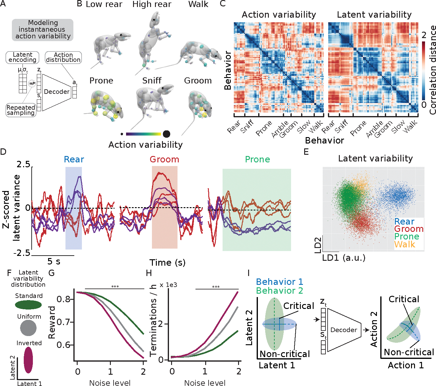
A) We estimate instantaneous action variability as the standard deviation of the set of actions obtained by resampling the latent space 50 times at every step. To avoid long-term temporal dependencies, simulations in this figure use a torque-actuated controller with a multi-layer perceptron decoder and a KL regularization coefficient of 1e-3. B) Action variability differs as a function of behavior (p < .001, one-sided permutation test; see methods). Each sphere corresponds to a single actuator; its color and size indicate its normalized action variability during the designated behavior. C) RDMs of action variability and latent variability across behaviors. D) Trajectories of six latent dimensions along which variability was differentially regulated across behavior. E) Scatter plot depicting the latent variability at single time points plotted on the first two linear discriminants for three behavioral categories. The population latent variability discriminates behaviors (p < .001, one-sided permutation test; see methods). F) Schematic depicting changes to the structure of latent variability (see text). G) The deviations from normal variability structure reduce the model’s robustness to noise (p < .001, one-sided Welch’s t-test) H) and termination rate (p < .001, one-sided Chi-squared test). Lines indicate significant differences between conditions. I) (Schematic) The latent variability is differentially shaped as a function of behavior to structure action variability in accordance with the minimal intervention principle.

To determine whether the virtual rodent’s actions exhibited structured variability, we estimated the instantaneous action variability at each timepoint (Fig. 5 A), and averaged across behavioral categories. As in biological controllers, the structure of variability across the model’s actuators showed a strong dependence on the behavior (i.e., the task) being performed (Fig. 5 B). However, unlike in biological controllers, signal-dependent noise cannot contribute to this structured variability as none of the sources of variability in the network were signal-dependent by construction. Consistent with action variability being controlled by the network’s latent variability, we found that their dissimilarity structure across behaviors were similar (Fig. 5 C), with individual latent dimensions expanding or contracting their variability as the virtual rodent performed different behaviors (Fig. 5 D). Indeed, the behavioral dependence was so strong that the latent variability alone was sufficient to identify the behavior enacted at any given time (Fig. 5 E). To relate the latent variability structure across behavior in the virtual rodent with the neural variability structure of real animals, we compared RDMs derived from the latent variability and the temporal variability of neural activity evaluated over a one second moving window (See methods). Intriguingly, the latent variability structure resembled that of the temporal variability of neural activity across behaviors (Extended Data Fig. 9 G–I), suggesting that the inverse dynamics models predict not only the structure of neural activity but also its variability.

To determine whether the structure of the virtual rodent’s latent variability afforded robustness in accordance with the minimal intervention principle, we changed it in two different ways. We made the variability across all dimensions of the latent encoding uniform and, in a different simulation, inverted the variability, i.e., quenching it in dimensions with normally high variability and vice versa (see methods) (Fig. 5 F). These deviations from the virtual rodent’s learned variability structure resulted in poorer imitation and more frequent failures at equal noise levels (Fig. 5 F–H), consistent with the system’s variability structure obeying the minimal intervention principle ⁷. To be clear, we do not suggest that the latent variability itself improves performance or robustness. In fact, models with stronger latent regularization, and thus greater latent variability, performed slightly worse in terms of imitation reward and robustness on the testing set (Extended Data Fig. 3 E–F). Instead, these results, coupled with the training objective (see Supplementary Discussion 2), show that the virtual rodent adaptively shapes latent variability to increase robustness according to behavioral demands (Fig. 5 I), affording robustness in the face of unquenchable noise. This structured variability emerges solely from latent variable compression, suggesting a link between mechanisms for robustness and generalizability (see also ^25,56).

Discussion:

How the brain achieves robust and flexible control of complex bodies has remained a puzzle in large measure due to the lack of expressivity in our models and their reductionist nature. Here, we address these limitations by taking a holistic approach to sensorimotor control that emphasizes embodiment, sensory feedback, stochastic control, and diverse behavior. Our approach reflects a belief that motor system function cannot be understood independent of the body it evolved to control or the behaviors it evolved to produce (Fig. 1A).

To demonstrate the utility of this approach, we developed a virtual rodent in which a fully configurable and transparent ANN controls a biomechanically realistic model of a rat in a physics simulator (See Supplementary Discussion 3). In constructing such a system, we needed to balance tractability, expressivity, and biological realism, both at the level of the biomechanical plant and its controller. In this work, we opted for the simplest model that could recapitulate the behavioral repertoire of the rat and predict the structure of neural activity in the brain across behavior. The result was a plant with point-torque actuation and a controller implementing inverse dynamics. Our simulations show that this level of model abstraction, which notably omits muscular actuation, is already sufficient to achieve our objectives. As we and others extend these biomechanical models to include whole-body musculoskeletal actuation, it will be interesting to probe the degree to which such increased biomechanical realism further informs our understanding of the neural control of movement.

To train the virtual rodents to replicate spontaneous behaviors of real rats (Fig. 2), we developed an imitation learning pipeline, MIMIC (Fig. 1 C–F). Remarkably, we found that the virtual rodents generalized to unseen movements across the entirety of our dataset with high fidelity and robustness (Fig. 2, Extended Data Fig. 3). In comparing the network activations to neural recordings in real rats performing the same behaviors, we found that our model explained the structure of recorded neural activity across a wide range of naturalistic behaviors better than any traditional representational model (Figs. 3–4). Because the virtual rodent’s ANN implements an inverse dynamics model, the observation that its network activations predict single-unit and population neural activity in DLS and MC more accurately than measurable features of movement or alternative control functions is consistent with these regions taking part in implementing inverse dynamics.

We believe that the improvements in predictivity relative to representational models result from incorporating bodily dynamics, including the influences of gravity, friction, inertia, and interactions between body parts. Note however, that one should ostensibly be able to find a combination of measurable representational features that predicts neural activity as well as our models. In fact, this is what our models do. They learn a nonlinear function, parametrized by a neural network, that transforms the kinematics of desired future movements into the dynamics required to achieve those kinematics. The network does this by encoding the physical realities of bodily control in its weights; i.e., it learns an inverse dynamics model. There are at least two major advantages of our approach relative to approaches based on representation. First, the models we train are causal - they are sufficient to physically reproduce the behavior of interest as opposed to merely describing it. Second, they place the emphasis on identifying the functions that brain regions implement as opposed to merely describing the flow of information.

Previous work in brain-machine interfaces ⁵⁷ and oculomotor control ⁵⁸ has similarly related neural activity in the motor system to inverse dynamics models. Our work extends these findings to the domain of full-body control and across a diverse behavioral repertoire. We note that a neural code consistent with inverse dynamics could reflect and support other processes, including motor learning ⁵⁹ or even different control functions. However, in our experiments, models trained to implement forward dynamics and sequential forecasting did not fare as well in predicting neural activity structure (Extended Data Fig. 9 A–F), although we note that these controls may differ from internal models (e.g. state estimation, forward dynamics models, etc.) implemented in a composite controller ⁶⁰. In future work, a more comprehensive understanding of the relationship between control functions and neural activity structure could be achieved by comparing the network activations of such composite controllers to neural recordings in brain regions believed to implement different internal models.

While noise is inherent to biological control, how the nervous system deals with it to ensure robustness and flexibility remains unclear ⁶¹. The minimal intervention principle speaks to this, explaining that controllers quench movement variability along dimensions relevant to performance ^7,51. By leveraging stochastic ANN controllers (Fig. 2 A), the virtual rodent allowed us to study the relationship between network variability and variability in motor output. Intriguingly, we found that the virtual rodent ‘brain’ regulated its latent variability to control action variability in accordance with the minimal intervention principle ⁷ (Fig. 5). The structure of variability emerged from training the network to balance latent variable compression, implemented to support generalization, and the ability to faithfully imitate over the training set (Supplementary Discussion 2). Thus, managing the trade-off between latent variable compression and motor performance ^25,56 may structure neural variability in ways that are distinct from previously hypothesized mechanisms like signal-dependent noise ⁵⁴ or energy constraints ⁷. Together, these results reveal a link between a computational mechanism for generalization (latent variable compression) and one for robustness in control (structured variability). That the virtual rodent’s latent variability predicts the structure of neural variability across behaviors in DLS and MC (Extended Data Fig. 9 G–I) further suggests that the brain may structure neural variability in accordance with these principles.

More generally, our results demonstrate how artificial controllers actuating biomechanically realistic models of animals can help uncover the computational principles implemented in neural circuits controlling complex behavior. We believe the potential of this approach is significant and untapped. Virtual animals trained to behave like their real counterparts could provide a platform for virtual neuroscience to model how neural activity and behavior are influenced by variables like feedback delays, latent variability, and body morphology that would otherwise be difficult or impossible to experimentally deduce. Inverse dynamics models trained to reproduce diverse and realistic behaviors could also be reused as low-level modules to promote naturalistic movement in neural networks trained to autonomously perform tasks, including those common in neuroscience research ^3,4. Similarly, since the ANNs controlling the virtual rodent are fully configurable, future iterations could aim to implement brain-inspired network architectures to improve performance and interpretability and probe the roles of specific circuit motifs and neural mechanisms in behaviorally relevant computations.

Methods

Data acquisition

Animals:

The procedures involved in the care and experimental manipulation of all animals were reviewed and approved by the Harvard Institutional Animal Care and Use Committee. Experimental subjects included seven female Long Evans rats, aged 3–12 months at the start of recording (Charles River).

Behavioral apparatus:

Animals moved freely in a cylindrical arena of 1 meter in diameter elevated on a custom-made wooden table. The circular base of the cylinder was made of green high-density polyethylene cutting board. The walls were 60 cm tall and made of a 1 mm thick clear polycarbonate sheet. The arena was surrounded by a commercial green screen to improve contrast between the animals and their surroundings. The arena was illuminated by two white LED arrays (Genaray SP-E-500B, Impact LS-6B stands) to aid kinematic tracking. To encourage movement, three to six Cheerios were hung around the arena using pieces of string such that they were within reach of the rats when rearing.

Videography:

Six high-speed 2 megapixel Basler Ace-2 Basic cameras (a2A1920–160160ucBAS) were equipped with 8mm lenses (Lens Basler 8 mm, C23–0824-5M, 2/3”, f/2.4, 5 MP) and placed surrounding the arena at regular intervals approximately 1.2 m from the center. Cameras were stabilized with SLIK PRO 700DX tripods. All camera shutters were controlled synchronously by a 50 Hz arduino hardware trigger via Phoenix Contact Sensor/actuator cables (SAC-6P-M AMS/3.0-PUR SH - 1522309). Images were transmitted via Basler USB 3.0 cables to an acquisition computer equipped with an Intel Core i9–9900K processor, a NVIDIA Quadro P4000, a NVIDIA Geforce GTX 1550 Super, and a Samsung 970 Evo M.2 SSD. We used the Campy camera acquisition software suite to encode videos from all cameras in real time ³⁵.

Calibration:

Cameras were calibrated using tools from the MATLAB 2020b (https://www.mathworks.com/downloads/web_downloads/) and OpenCV-Python (4.4.0.46) (https://pypi.org/project/opencv-python/#history) camera calibration libraries. For intrinsic calibration, we used the MATLAB Single Camera Calibrator App with a checkerboard calibration pattern to estimate the camera parameters for each camera individually. For extrinsic calibration we placed the same checkerboard used for intrinsic calibration in the center of the arena, took a picture from all cameras, detected checkerboard corners in all images using the functions in OpenCV-Python calibration library, and estimated the rotation and translation vectors for each camera using MATLAB’s extrinsic calibration functions. Calibrations were checked periodically to ensure that the cameras had not been accidentally disturbed between recordings. In practice, we found the recording apparatus to be stable enough that calibrations would remain accurate for months at a time.

Electrophysiology:

Microdrive construction and surgical procedures for tetrode implantation followed previously described protocols ⁶², with slight modifications to accommodate 128-channel recordings. Notably, an array of 32 tetrodes was manually connected to a custom-designed headstage (made of 2 RHD2164 ICs from Intan Technologies), rather than the 16 tetrodes used in previous designs. All implants were in the right hemisphere. Target coordinates were 0 mm AP +4.25 mm ML −4 mm SI for the DLS, and +1 mm AP + 1 mm ML −1 mm SI for MC relative to bregma. MC targets were chosen to match the median recording location of MC recordings by Mimica et al. ³⁶. In one MC implant, the target site was moved by approximately +1 mm AP and + 1 mm ML to avoid a blood vessel. We occasionally lowered the drive by approximately 80 μm, 0–4 times over the course of the experiments. Recordings were conducted using the Intan RHX2000 acquisition software. Electrophysiological and video data were synchronized by passing the video hardware trigger signal through the acquisition FPGA (Opal Kelly XEM6010, Xilinx Spartan-6 FPGA) that interfaced with the headstage. One animal implanted in MC yielded no neurons, and was thus excluded from electrophysiological analyses.

Recording protocol:

Single-housed rats were manually placed in the arena at the beginning of a recording session and left alone and undisturbed for two or three hours. All recordings were performed in the absence of experimenters in a closed room with minimal noise and began at approximately the same time every day. Animals were recorded daily for a minimum of 28 days and a maximum of 63 days. The arena floor and walls were cleaned with 70% ethanol after every recording session and allowed to dry for at least 30 minutes before further use. In total, the dataset spans 607 hours of simultaneous electrophysiology and videography (353.5 hours DLS and 253.5 hours MC).

Histology:

At the end of the experiment, we performed an electrolytic lesion of the recording site by passing a 30 μA current through the electrodes. For two animals implanted in MC, we were unable to perform a lesion as the headstages came off unexpectedly. The location of these implants was verified based on scarring caused by the implant. After lesioning, animals were euthanized (100 mg/kg ketamine; 10 mg/kg xylazine) and transcardially perfused with 4% paraformaldehyde in 1x PBS. We then extracted the brains and placed them in 4% paraformaldehyde for two weeks. Brains were sectioned into 80 μm slices using a vibratome (Vibration Company Vibratome 1500 Sectioning System), mounted the slices on microscope slides, and stained with Cresyl-Violet. We imaged the slides using an Axioscan slide scanner and localized the recording site by the electrolytic lesions.

Data processing

3D Pose Estimation:

We used DANNCE version 1.3 to estimate the 3D pose of the animal over time from multi camera images. Pose estimation with DANNCE consists of two main steps: center of mass (CoM) detection and DANNCE keypoint estimation.

CoM network training:

We used Label3D ³⁵ to manually label the rat CoM from multi camera images in 600 frames spanning 3 animals. Frames were manually selected to span the range of locations and poses animals assume when in the arena. CoM networks were trained as described previously ³⁵.

DANNCE network training:

We again used Label3D to manually label the 3D positions of 23 keypoints along a rat’s body. The dataset consisted of over 973 frames manually selected to sample a diverse range of poses from four different animals over 8 different recordings. We finetuned a model previously trained to track keypoints in the Rat7M (https://doi.org/10.6084/m9.figshare.c.5295370.v3) dataset on our training set, as in earlier work ³⁵. Notable modifications to this procedure included two methods for data augmentation and a modified loss function. The first data augmentation method is mirror augmentation, which effectively doubles the dataset size by inverting the 3D volumes generated from multi camera images along the X-axis (parallel to the ground) and swapping the 3D positions of bilaterally symmetric keypoints. The second is view augmentation, which randomly permutes the order that images from different cameras are fed into the network. Finally, we used an L1 loss function rather than the original L2 loss. We include a list of relevant DANNCE parameter specifications in Supplementary Table 2.

Evaluation:

DANNCE performance was quantified using a dataset of 50 manually labeled frames randomly selected from a recording session that had not been included in the training set. To estimate intra-labeler variability, the same 50 frames were re-labeled by the same person one month after the initial labeling. We report the keypoint error between manual labels and DANNCE predictions up to a Procrustes transformation without scaling.

Compute resources:

CoM and DANNCE models were trained and evaluated using computational resources in the Cannon High Performance Cluster operated by Harvard Research Computing. These included a mixture of NVIDIA hardware including GeForce GTX 1080 Ti, GeForce RTX 2080 Ti, Tesla V100, A40, and A100 Tensor Core GPUs.

Skeletal model:

We previously developed a skeletal model of a rat that matches the bone lengths and mass distribution of Long Evans rats ¹. The model has 74 degrees of freedom (DoF) and defines parent-child relationships between body parts through an acyclic tree that starts with the root (similar to the center of mass) and branches to the extremities. The pose of the model consists of 3 Cartesian dimensions specifying the position of the root in space, 4 dimensions specifying the quaternion that captures the orientation of the model relative to the Cartesian reference, and 67 dimensions that specify the orientations of child body parts relative to their parent’s reference frame. The model has 38 controllable actuators that apply torques to specific joints. To help imitate rearing, we increased the range of motion of the ankle and toe joints to [−.1, 2.0] and [−.7, .87] radians. The model is equipped with a series of sensors, including 1) a velocimeter, 2) an accelerometer, 3) a gyroscope, 4) and force, torque, and touch sensors on its end effectors.

Skeletal registration:

We used a custom implementation of STAC ⁴⁴ to register the skeletal model to the DANNCE keypoints. Briefly, STAC uses an iterative optimization algorithm to learn a set of 3D offsets that relate different sites along the skeletal model to DANNCE keypoints (m-phase), as well as the pose of the model that best reflects the keypoints at each frame given the set of offsets (q-phase). To ensure consistent relationships between keypoints and model sites across different poses, the offsets corresponding to keypoints closest to a body part were expressed in the reference frame of the parent body part.

In the m-phase, we optimize the offsets using L-BFGS-B over a dataset of 500 frames to minimize the mean squared error between the true keypoints and fictive keypoints derived from applying the offsets to the posed model. In the q-phase we optimize the pose of the model using least-squares optimization over the same set of frames to minimize the same objective while keeping the offsets fixed. At each step of the pose optimization, we reposition the model and compute new positions of the fictive offsets via forward kinematics in MuJoCo.

As the dataset totaled 607 hours of data sampled at 50 Hz, the registration algorithm needed to be efficient. To speed up the q-phase, we separately optimized the pose of different body parts rather than optimizing over the full body pose. First, we initialize the model’s root position as the position of the middle spine keypoint and optimize only the 7 DoF specifying the Cartesian position and quaternion of its root. We next optimize the quaternions of the root, trunk, and head to match keypoints along the head and trunk of the animal. Finally, we individually optimize each limb. In subsequent frames, we initialize the model’s pose using its pose in the previous frame.

For each animal, we independently estimated the offsets using the procedure described above. We accounted for differences in animal size by isometrically scaling the model by a scaling factor manually determined via a visual comparison of models overlain on images of the rats. We found this procedure to be more robust, faster, and produce comparable results to a direct optimization of the scaling factor when learning offsets. In practice, we found that running the iterative optimization three times produced reasonable offsets that could be used to estimate the skeletal pose in new keypoint data.

To infer the skeletal pose of an entire recording session, we ran the q-phase optimization a final time using the set of offsets learned during training. To improve inference speed, we divided the session into contiguous 20 second chunks and ran the q-phase optimization in parallel on Harvard Research Computing’s Cannon HPC.

Behavioral segmentation:

We automatically identified stereotyped behaviors throughout our recording sessions using an unsupervised feature extraction and clustering approach described previously ^40–43. We extracted a high-dimensional feature vector capturing the multiscale dynamics of the animal’s keypoints over time. The vector was composed of three types of features. The first was the height of the keypoints from the floor, smoothed using a 60-ms median filter. The second was the keypoint velocities, estimated using the finite differences method on smoothed (100-ms, median filter) keypoint trajectories. The third was a multiscale time-frequency decomposition of the rat’s pose, obtained by computing a pairwise distance matrix between keypoints for all frames in the smoothed keypoint trajectories, decomposing the matrix into its top 20 principal components, and applying a continuous wavelet transform to each principal component with frequencies ranging from 0.5 to 20 hz.

To aid in identifying diverse stereotyped behaviors, we implemented a sampling and clustering procedure. For each session, we subsampled the feature vector by a factor of 20 and embedded it into a 2-dimensional space using t-distributed stochastic neighbor embedding. We next clustered the resulting space using hierarchical watershed clustering, and uniformly sampled 500 samples across the clusters. Samples from each session were compiled into a single set and clustered to automatically assign behavioral categories to individual frames using k-means clustering (K=100). The resulting cluster centroids were then used to classify the remaining frames in the original dataset.

Spike sorting:

For each animal, the raw neural data from all sessions was sorted using an improved implementation of Fast Automated Spike Tracker (FAST) ⁶². While the majority of the sorting process remains unchanged between the implementations, there are three relevant modifications.

Feature extraction:

We applied a β-distribution (β=100) weighting transform to the spike waveforms to more heavily weigh the values near the spike peak. We next spectrally decomposed the waveforms using a discrete wavelet transform with a Symlets 2 wavelet. Finally, we applied Principal Components Analysis on the wavelet coefficients, retaining only the first 10 components.

Clustering:

We identified putative single units using ISO-split ⁶³ rather than superparamagnetic clustering. We used an iso-cut threshold of .9, a minimum cluster size of 8, 200 initial clusters, and 500 iterations per pass.

Linking:

To sort our long-term recordings, we clustered the feature-transformed data spanning chunks of approximately 1 hour using ISO-split, and linked clusters across chunks using a variation of the segmentation fusion algorithm detailed in FAST. The relevant modification was using the Komolgorov-Smirnov criterion from ISO-split to link similar neurons across recording sessions.

Criteria for unit selection:

After manual curation, we used several summary statistics to further assess the quality of putative single units. For encoding analyses, we excluded units with an isolation index ⁶² less than .1, and a proportion of interspike interval violations greater than .02. For single-unit analyses, we excluded units with average firing rates less than .25 Hz and a total recorded duration that failed to span the entirety of the session in which they were measured. For population analyses, we excluded units with average firing rates less than .05 Hz and those with total recorded durations that failed to span the entirety of the session in which they were measured (2092 putative single units, 1249 DLS, 843 MC). For all analyses, spike times were binned into 20 ms bins.

Model training

Training set:

The training data for MIMIC controllers consists of contiguous trajectories of a high-dimensional state vector describing the real animal’s movement. Features in this vector were derived from the skeletal registration and are as follows: freejoint Cartesian position, root quaternion, joint quaternions, center of mass (CoM), end effector Cartesian position, freejoint velocity, root quaternion velocity, joint quaternions velocity, appendage Cartesian positions, body Cartesian positions, and body quaternions. Velocities were estimated with the finite differences method.

We automatically identified a collection of 5-second clips containing a wide range of behaviors spanning our behavioral embedding. We found it necessary to prioritize behaviors in which the animal was moving to prevent the model from converging to local minima where it would remain still. We visually verified the quality of each clip by removing clips in which the animal did not move or seemingly assumed physically implausible poses from errors in tracking or registration. In the end we used a dataset of 842 clips.

Imitation task:

We used an imitation task similar to previous works on motion capture tracking ^5,64,65, and most closely resembling CoMic ³. The task has four major considerations: initialization, observations, reward function, and termination condition.

Initialization:

Episodes were initiated by randomly selecting a starting frame from the set of all frames across all clips, excluding the last ten frames from each clip. The pose of the rat model was initialized to the reference pose in the selected frame.

Observations:

The model received as input a combination of proprioceptive information, motion and force sensors, and a reference trajectory. These include the actuator activation, appendage positions, joint positions, joint velocities, accelerometer data, gyroscope data, touch sensors at the hands and feet, torque sensors at the joints, velocimeter data, tendon position, tendon velocities, and the reference trajectory. The reference trajectory is defined as the set of states visited by the real animal in a short time window ranging from 20 ms to 200 ms in the future (the majority of models had a time window duration of 100 ms). At each timepoint, the kinematics of the reference trajectory was represented relative to the current state of the model in Cartesian and quaternion representations. Given the short timescales of the reference trajectory, we believe our models are most appropriate for interpreting the short-timescale dynamics involved in motor control, rather than the long term organization of behavior.

Reward functions:

As in previous work on motion capture tracking ^3,5,64, we treat the imitation objective as a combination of several rewards pertaining to different kinematic features. The rewards consist of four terms that penalize deviations between the reference trajectory and the model’s kinematics and one term that regularizes actuator forces.

The first term, $r_{com}$, penalizes deviations in the positions of the CoM between the reference and model.

$$r_{com}=\exp \left(-100{‖p_{com}-p_{com}^{ref}‖}^2\right)$$

Where $p_{com}$ and $p_{com}^{ref}$ are the CoM positions for the model and reference, respectively. Only spatial dimensions parallel to the ground were included to avoid the ambiguity in CoM height between isometrically scaled versions of the model used for skeletal registration and the unscaled versions of the model used in training.

The second term, $r_{vel}$, penalizes deviations in the joint angular velocities between the reference and model.

$$r_{vel}=\exp \left(-.1{‖q_{vel}-q_{vel}^{ref}‖}^2\right)$$

Where $q_{vel}$ and $q_{vel}^{ref}$ are the joint angle velocities of the model and reference, respectively, and the difference is the quaternion difference.

The third term, $r_{app}$, penalizes deviations in the end effector appendage position between the reference and the model.

$$r_{app}=\exp \left(-400{‖p_{app}-p_{app}^{ref}‖}^2\right)$$

Where $p_{app}$ and $p_{app}^{ref}$ are the end effector appendage positions of the model and reference, respectively.

The fourth term, $r_{quat}$, penalizes deviations in the joint angles of the model and reference.

$$r_{quat}=\exp \left(-2{‖q_{quat}-q_{quat}^{ref}‖}^2\right)$$

Where $q_{quat}$ and $q_{quat}^{ref}$ are the joint angles of the model and reference, respectively.

The fifth term, $r_{act}$, regularized the actuator forces used across the agent’s actuators.

$$r_{act}=-0.015\frac{1}{D}\sum _{i=1}^D{a}_i^2$$

Where $D$ is the number of controllable actuators and $a_i$ is the actuator force of the $i$th actuator

Termination condition:

Episodes were automatically terminated when the model’s movements substantially deviated from the reference. Specifically, episodes terminated when

$$1-\frac{1}{\tau }\left({‖b_{pos}-b_{pos}^{ref}‖}_1+{‖q_{pos}-q_{pos}^{ref}‖}_1\right)<0$$

Where $\tau$ corresponds to the termination threshold, $b_{pos}$ and $b_{pos}^{ref}$ correspond to the body positions of the model and reference, and $q_{pos}$ and $q_{pos}^{ref}$ correspond to the joint angles of the model and reference with the difference being the quaternion difference. We used a $\tau$ value of .3 in all experiments.

Training:

Models were trained using multiple objective value maximum a posteriori policy optimization (MO-VMPO) ⁶⁶. In this setting, MO-VMPO trains a single policy to balance five objectives corresponding to each of the five reward terms. The relative contribution of each objective is specified by a vector, $ϵ$, with a single element per objective. We set ${ϵ}_{com}=0.01,{ϵ}_{app}=0.01,{ϵ}_{vel}=0.01,{ϵ}_{quat}=0.01$, and ${ϵ}_{act}=0.0001$. For all models, we used a batch size of 256, an unroll length of 20, and a discount factor of 0.95. In the MO-VMPO E-steps, we use the top 50% of advantages ⁶⁷. In the policy distillation step, we set the KL bounds for the policy mean to 0.1, and the KL bounds for the policy covariance to $1e^{-5}$. We initialized all Lagrange multipliers in MO-VMPO to 1, with minimum values of $1e^{-8}$. We used Adam ⁶⁸ for optimization with a learning rate of $1e^{-4}$. Models were trained using 4000 actors, 32 cachers, and a TPUv2 chip. A typical model trained for 2–3 days.

Model Architectures

An overview of model architectures is included in Supplementary Table 3.

Reference encoder:

All architectures featured the same reference encoder. We used the reference trajectory for the following five timesteps and proprioceptive observations at the current timestep as inputs to the reference encoder. The encoder consisted of a two-layer densely-connected multi-layer perceptron (MLP) with 1024 hidden units in each layer and hyperbolic tangent activation functions, using layer norm. The final layer of the encoder produced two 60-dimensional vectors that were passed through linear activation functions to respectively parametrize the mean, $\mu$, and log standard deviation, $\sigma$, of the stochastic latent representation.

MLP value function:

For MLP networks, the critic was composed of a two-layer MLP with 1024 hidden units, followed by one additional one-layer MLP for each objective. It received the same inputs as the reference encoder.

LSTM value function:

For LSTM networks, the critic was composed of a single LSTM with 512 hidden units, followed by one additional one-layer MLP for each objective. It received the same inputs as the reference encoder.

Latent regularization:

As in CoMic ³, we append an additional Kullback-Liebler (KL) divergence loss term to the MO-VMPO policy distillation objective that regularizes the latent embedding using a standard Gaussian prior,

$$\beta {\mathbb{E}}_{\pi }\left[KL\left(\pi \left(z_t\right|s_t,s_t^{ref}\right)\right.‖𝒩\left(0,I\right))]$$

with the scalar parameter $\beta$ controlling the strength of the regularization. We additionally impose a one-step autoregressive prior, AR(1), described by

$$z_{t+1}=\alpha z_t+\sigma ϵ,ϵ~𝒩\left(0,I\right)$$

Where $\alpha$ is the contribution of the autoregressive term. For models with autoregressive priors we use $\alpha$ to .95, and for those without autoregressive priors, we set $\alpha$ to zero.

MLP Decoder:

The MLP decoder was composed of a two-layer MLP with 1024 hidden units.

LSTM Decoder:

The LSTM decoder was composed of two stacked LSTMs with 512 and 256 hidden units respectively.

Action type:

We trained models with two types of actions. The first was position-controlled action, in which model outputs denoted the desired position of each controllable actuator. The forces required to achieve those positions were then computed via inverse kinematics to actuate the model appropriately. The second was torque-controlled action, in which the model directly produced torques at each actuator.

Reference trajectory duration:

In one experiment (Extended Data Fig. 11), we trained five inverse dynamics models that varied in the duration of the reference trajectory (20, 40, 60, 100, or 200 ms). The models all featured torque actuation, a LSTM decoder, and a KL regularization coefficient of 1e-4.

Body modifications:

In two separate experiments (Extended Data Fig. 12, 13), we trained inverse dynamics models to control modified versions of the virtual rodent body. These modifications were designed to influence the dynamics of movement without requiring changes in the kinematics of movement. In a ‘mass scaling’ experiment, we uniformly scaled the masses of all body parts of the virtual rodent body from half to twice the standard mass. In a ‘relative head scaling’ experiment we scaled the mass of the head relative to the mass of the rest of the body from half to twice the standard ratio. In both experiments, we trained inverse dynamics models with torque actuation, a LSTM decoder, and a KL regularization coefficient of 1e-4 to control the different modified bodies, and evaluated their performance on held-out data controlling the bodies on which they were trained.

Model inference

Rollout:

To evaluate the models on new data, we used the postural trajectories obtained from STAC as reference trajectories. At each frame, the model would accept its current state and the reference trajectory for the following frames and generate an action. After applying forward kinematics, this action would result in the state at the next frame, closing the sensorimotor loop. In the initial frame, the model’s state was initialized to the state of the real animal. For the encoding and representational similarity analyses, we disabled the noise at the action periphery and the sampling noise in the stochastic latent space. For analyses of the model’s latent variability, these sources of noise remained enabled.

At each frame, we recorded physical parameters related to the model’s state, activations of several layers of the ANN controllers, and the fictive reward. The physical parameters included STAC-estimated keypoints, quaternion forces experienced at all joints, quaternion positions, velocities, and accelerations, and the cartesian positions of all joints. The recorded ANN layers included the latent mean and log standard deviation, the latent sample, all LSTM hidden and cell states, and the action.

To aid in comparing the network’s activity to neural activity, we maintained the termination condition employed during training. This decision had two effects. First, it maintained that the model’s behavior was within a reasonable range of the true behavior. Second, it ensured that the state inputs to the model were within the distribution observed during training, and thus prevented the network activity from behaving unpredictably. For all analyses, we excluded the .2 seconds preceding or following initialization or termination frames.

As this rollout process is serial and limited by the speed of the physical simulation, evaluating long sessions is time consuming. To improve inference speed, we divided all recordings into 50 s chunks and evaluated models on each chunk in parallel, using 1 CPU core per chunk.

Alternative control models

To compare the structure of neural activity across behavior to functions other than inverse models, we use a dataset of state-action pairs obtained from MIMIC model rollouts when imitating natural behavior to implement forward and sequential forecasting models in ANNs using supervised learning (Extended Data Fig. 10 A–F). States were parametrized by the model’s quaternion pose, while actions were parametrized by the model’s action. Forward models were trained to predict the sensory consequences of motor actions, transforming the state and action for the current frame into the state of the next frame. Sequential forecasting models were trained to predict future states from past states. We varied the number of frames spanning the past-state vector from 1 to 5 to test the influence of longer context while maintaining parity with the window size of the inverse models.

The encoders and decoders for both models were composed of multi-layer perceptrons with three hidden layers of 1024 units each, with leaky rectified linear unit activation functions ⁶⁹. All models featured β-weighted conditional latent bottlenecks of equal dimensionality to those of the inverse dynamics models (60), with a β value of .01. The objective was to minimize the mean-squared error of the target.

While we believe that comparisons to models trained via supervision is valuable, it is possible that the representations of models trained via reinforcement to implement alternative control functions may differ from those trained through supervision. This question could be resolved in future work via the integration of multiple control functions into composite controllers trained via reinforcement.

Encoding analyses

Feature set:

We used Poisson generalized linear models (GLMs) with a log link function ⁷⁰ to predict the spiking of putative single units in DLS and MC from measurable movement features, features inferred from physical simulation in MuJoCo, and the activations of ANN inverse controllers. The measurable features included aligned 3D keypoint positions and velocities and joint angular positions and velocities, spanning the entire body. Dynamic features inferred from MuJoCo included the forces experienced at each joint, and accelerometer, velocimeter, and touch sensors. Finally, the ANN activations included the activations of every layer of the inverse dynamics models, considered independently.

To ensure that the models were trained to predict movement-related activity rather than activity during sleeping or resting, we focused only on frames in which animals were moving. To estimate moving frames, we smoothed the keypoint velocities estimated via finite differences with a 5 frame median filter and identified frames in which the average smoothed keypoint velocity was above a threshold of .07 mm/frame. We then estimated sleeping frames as the set of frames resulting from the application of 20 iterations of binary closing (binary erosion followed by binary dilation) and 500 iterations of binary opening (binary dilation followed by binary erosion) to the vector of non-moving frames.

For all features, we used data from a temporal window containing the five surrounding samples to predict the number of spikes in a given bin. In general, increasing the window size improved model predictivity up until five frames. We also trained models over a range of offsets (−1000 ms to 300 ms in 100 ms intervals) that shifted the temporal relationship of neural activity relative to each feature.

Regularization:

As many of the features are high-dimensional, we took several steps to counter overfitting. First, we used principal components analysis to decrease the effective dimensionality of our feature sets, retaining only the components required to explain 90% of the variance in the temporal windows for each feature. To further address overfitting, we used elastic net regularization with an L1 weight of .5 and an $\alpha$ value of .01. Qualitatively, results were not sensitive to changes in these parameter choices.

Cross validation:

We trained GLMs using a five-fold cross validation scheme. We first divided the spiking, movement, and ANN data spanning the duration of a unit’s recording into 4-second chunks which were randomly distributed into ten folds. We trained GLMs using training data from nine of the folds and evaluated their performance on testing data from the remaining fold, training a single model for each combination of training and testing sets. We use the cross-validated log-likelihood ratio (CV-LLR) and deviance-ratio pseudo-$R^2$ to quantify model predictivity, the performance of a model in predicting spike counts in the testing set.

Hypothesis testing: We defined the most predictive feature for a given unit as the feature with the highest average CV-LLR. To identify units for which the features had low predictivity, we used a one-sided Wilcoxon signed-rank test to assess whether the CV-LLRs for each unit and each feature sufficiently deviated from zero. Units with a confidence score greater than .05 with Bonferroni correction for multiple comparisons were labeled as unclassified.

Representational similarity analysis

We used representational similarity analysis (RSA) to compare the representational structure of neural activity in DLS and MC across behaviors to measurable features of movement, dynamic features inferred from physical simulation, and the activations of ANN inverse controllers. RSA consists of three broad steps: feature vector estimation, representational dissimilarity matrix (RDM) estimation, and RDM comparison.

Feature vector estimation:

We first applied principal components analysis to each feature, retaining only the components required to explain 95% of the total variance. For each session, we used the behavioral labels from our automated behavioral segmentation, applied a 200 ms iterative mode filter to mitigate short-duration bouts, and divided samples from each feature into behavioral categories. To eventually achieve an unbiased estimate in the dissimilarity between behavioral categories for a given feature, we divided data into two partitions for each behavior, with odd instances of the behavior comprising the first partition and even instances of the behavior comprising the second partition. For each partition, we computed the average feature vector across all samples.

We excluded frames in which the animal was sleeping and frames in the 40 samples surrounding the initiation or termination of the model’s imitation episodes. We only included sessions in which a minimum of 10 simultaneously recorded neurons were present throughout the entire duration of the session, sessions in which a minimum of 70% of the total behavioral categories were expressed, and sessions in which there was a minimum of 30 minutes of movement.

RDM estimation:

We used rsatoolbox 3.0 to perform RDM estimation using the cross-validated squared Mahalanobis distance (crossnobis dissimilarity) ^71–73 with the feature vectors from the behavioral partitions described above. This produces a RDM for each feature and each session. While the models’ conditional latent bottlenecks naturally suggest calculation of RDMs using distance metrics for distributions, such as the symmetric KL-divergence, it was challenging to compare these metrics across features for which we do not have parameterized probability distributions. Thus, we chose to separately analyze the latent means and scales, as well as all other features, using crossnobis dissimilarity.

RDM Comparison:

For each feature we computed the average RDM across sessions and compared RDMs across features and subjects using the whitened unbiased cosine similarity ^71,72.

Motor variability analyses

Estimating instantaneous motor variability:

We modified the normal inference procedure to estimate the instantaneous motor variability of the model at each timestep. Rather than disabling the latent variability, we generated 50 latent samples from the latent distribution at each frame. We then evaluated the decoder for each sample to estimate the distribution of actions that emerged from a given latent distribution. We use the standard deviation across the distribution of actions for each actuator as the instantaneous estimate of actuator variability.

To assess the significance of the predictivity of action variability and latent variability on behavior, we performed a permutation test. For each of 1000 iterations, we trained a logistic regression classifier using balanced class weights to predict the behavioral category from the vector of action standard deviations or latent standard deviations at each timepoint. We also trained another logistic regression classifier using randomly permuted category labels. The performance of both classifiers were evaluated with 5-fold cross validation, using the class-balanced accuracy as a performance metric.

Variability perturbations:

We further modified the inference procedure to perturb the structure of latent variability. Our perturbation involved varying the structure of the latent variability and clamping the total variability of the latent space at each timepoint. We considered three different structures for the latent variability. The first was a standard variability structure, in which no changes were made to the latent distribution. The second was a uniform variability structure in which each dimension of the latent space was set to equal variance for every frame. The third was an inverted variability structure that was constructed as follows. In each frame the latent dimensions were ranked according to their latent standard deviation. The standard deviations were then reassigned in inverse rank order such that the dimensions with the highest variability were assigned low variability and vice versa. To clamp the variability at a particular noise level, we multiplied the transformed latent variability vector by a scalar value such that the total variability across all dimensions in the latent space equaled the desired noise level for every frame of the simulation.

To evaluate the performance of models undergoing variability perturbations, we defined a fictive reward term to combine the multiple MO-VMPO objectives into a single scalar value. The fictive reward was adapted from objective functions in previous work ³ and was defined by:

$$.4r_{com}+2r_{vel}+.15r_{app}+.35r_{quat}$$

Estimating instantaneous neural variability:

While the parametrizations of variability in latent variable models can be easily recorded, directly measuring instantaneous variability in neural activity is not possible. To approximate a measure of instantaneous neural variability, we computed a sliding-window variance estimate using a 1-second window on the binned spike counts of each neuron. In lieu of more sophisticated approaches that can estimate latent variability structure of neural populations across behavior and at the months-long recording scale, we believe that our approach serves as a reasonable approximation of neural variability structure.

Extended Data

Extended Data Figure 1. Recording neural activity in freely behaving rats.

A) Schematic of custom 128-channel tetrode drive. B) Tetrodes record electrical events of several putative neurons from the DLS or MC. Shown are recordings from a tetrode in DLS. C) Individual putative cells are extracted based on their unique spike waveforms using a custom spike-sorting software, FAST. D) Tetrodes allows for the recording of hundreds of putative single units simultaneously. E-F) Representative examples of Nissl-stained brain slices from animals with electrophysiological implants in DLS and MC. Red ellipses indicate the lesions remaining from the tetrode implants. G) Dorsal view denoting the position of implants for DLS and MC. The position of the implant with the dashed circle could not be verified with histology as the recording headstage was dislodged prior to electric lesion. The position was instead estimated using scarring at the cortical surface and the recorded depth of implantation. The other implants were verified with electric lesions or scarring from the implant tip. H) Coronal plane indicating the location of implants in the DLS across 3 animals. I) Coronal plane indicating the location of implants in MC across 3 animals.

Extended Data Figure 2. High fidelity 3D pose estimation and skeletal registration.

A) In DANNCE, a 3D U-Net processes multi-view images to estimate the positions of 23 3D keypoints across the rat’s body. B) DANNCE keypoint estimates show high concordance with manual annotations, deviating from manual labels to a similar degree as repeated manual annotations of the same testing frames. C) Visualization of median DANNCE keypoint discrepancy relative to manual annotation. Gray circles indicate the bounds of the sphere with radius equal to the median keypoint discrepancy for each keypoint. D) Schematic depicting the relevant variables in STAC. STAC operates by jointly optimizing a set of offsets relating the skeletal model to different keypoints and the pose of the model in each frame. E) STAC registration is highly accurate across body parts and F) across different behaviors. For all boxplots in this figure, colored lines indicate the median, boxes indicate the interquartile range, and whiskers indicate the 10th and 90th percentiles.

Extended Data Figure 3. Comparing imitation performance for held-out data across different classes of control networks.

A) The proportion of episodes exceeding a given duration for the four classes of controllers. Results for each class are averaged across models with all KL regularization coefficients for that class. B) Violin plots showing the distribution of rewards by each model class on the held-out testing set. Models with LSTM decoders outperform other classes. C) Average reward as a function of the center of mass speed for each class of controller. LSTM models outperform other model classes across all speeds, but especially at slow speeds. D) Box plots denoting the distribution of rewards for each model class as a function of behavior category. LSTM models outperform other classes across all behavior, but especially those with slow center of mass speed. White lines indicate the median, box limits indicate the interquartile range, box whiskers indicate the 10th and 90th percentiles. E) The proportion of episodes exceeding a given duration for models with LSTM decoders across all KL regularization coefficients. Models with higher KL regularization are generally less robust than those with lower KL regularization, consistent with an increase in latent noise. F) Violin plots denoting the distribution of rewards on held-out natural behavior for each model as a function of KL regularization. Increasing the KL regularization coefficient marginally decreases the reward distribution of the models. White lines indicate the median. G) We trained five models with different reference window lengths using an LSTM decoder with a KL regularization of 1e-4. Violin plots denote the distribution of rewards on held-out natural behavior for each model. Models with reference windows of length 5 or shorter exhibit comparable performance, while a reference window of 10 exhibits poorer performance. Gray lines indicate the quartiles. H) The proportion of episodes exceeding a given duration. Models with longer reference window length are generally more robust than those with shorter reference window lengths, with the most robust model being that with a reference window length of 5. Shaded regions indicate the standard error of the mean over sessions. I) The distribution of joint angles during imitation closely match those of STAC-registered skeletal models during imitation. Data is from a model with an LSTM decoder and a KL regularization of 1e-4. Box centers indicate the median, box limits indicate the interquartile range, box whiskers indicate the maximum or minimum values up to 1.5 times the interquartile range from the box limits.

Extended Data Figure 4. Neurons in the DLS and MC encode posture across many body parts to a degree consistent with previous reports during unrestrained behavior.

A, C) Proportion of neurons in DLS and MC best predicted by each feature class. B, D) Violin plots showing the distribution of cross-validated log-likelihood ratios (CV-LLR) of GLMs trained to predict spike counts using different feature classes. E, F) Box plots showing the distribution of deviance-ratio pseudo r-squared values of GLMs trained to predict spike counts using different feature classes. White lines indicate the median, boxes indicate the interquartile range, and whiskers indicate the 10th and 90th percentiles. G, H) Empirical cumulative distribution functions denoting the proportion of neurons in DLS and MC with peak GLM predictivity below a given pseudo r-squared value. The distributions resemble previous reports in rats during spontaneous behavior ⁴².

Extended Data Figure 5. Encoding properties are similar across striatal cell types.

A-C) Proportion of neurons in DLS and MC best predicted by each feature class for each cell type. D-F) Box plots showing the distribution of cross-validated log-likelihood ratios relative to a mean firing rate model for GLMs trained to predict spike counts using different feature classes. White lines indicate the median, boxes indicate the interquartile range, and whiskers indicate the 10th and 90th percentiles. G-H) Comparison of the best computational feature derived from the network and representational feature GLM CV-LLRs for each neuron. GLMs based on the inverse dynamics models (computational features) outperform those based on representational features for the majority of classified neurons for all cell types (p < .001, permutation test).

Extended Data Figure 6. Neurons in the DLS and MC encode future movement during natural behavior.

We trained GLMs to predict neural activity from measurable features of movement and from features of the ANN controllers while introducing time lags ranging from −1000 ms to 300 ms between neural activity and the features. A) Histograms depicting the distribution of time lags for maximally predictive GLMs when using joint angle predictors. Time lags less than zero correspond to neurons whose future movements better predict neural activity (premotor), while time lags greater than zero correspond to neurons whose past movements best predict neural activity (postmotor). B) CVLLR relative to models trained with a time lag of 0 ms averaged across neurons. Shaded regions indicate the standard error of the mean. The peak average CVLLR occurs at −200 ms for all cell types. C, D) Same as A-B, except using features from the inverse dynamics model (LSTM hidden layer 1) as GLM predictors for a model with an LSTM decoder and a KL regularization of 1e-4. Peak predictivity occurs closer to a time lag of zero, consistent with the network’s representation of desired future state and inverse dynamics. E,F) Same as A-B for neurons in MC. G, H) Same as C-D for neurons in MC.

Extended Data Figure 7. Comparing imitation performance and neural predictivity of models trained to control bodies of different masses.

A) We trained five models with an LSTM decoder and a KL regularization of 1e-4 to control bodies of different masses. Violin plots denote the distribution of rewards on held-out natural behavior for each model. Several models controlling bodies with masses other than the standard mass exhibited reduced performance. White lines indicate medians. B) The proportion of episodes exceeding a given duration. Shaded regions indicate S.E.M across individuals. C-D) Box plots depicting the distribution of cross-validated log-likelihood ratios across neurons of GLMs trained to predict neural activity from network features. The CVLLR for each neuron is expressed relative to the likelihood of a GLM trained to predict neural activity using network features from the standard mass model. Values greater than zero imply a model more predictive of neural activity than those derived from the standard mass model, and vice versa. White lines indicate the median, box limits indicate the quartiles, whiskers indicate the 10th and 90th percentiles. Stars indicate that a greater proportion of neurons are better predicted by GLMs trained using features from the standard mass model than from the alternative mass model (Bonferroni corrected, α = .05, permutation test). E-F) Average WUC similarity between RDMs derived from network layers and neural activity in DLS or MC. Error bars indicate S.E.M across individuals. Arrows indicate significantly different similarity distributions across animals (Benjamini-Hochberg corrected, false discovery rate α = .05, one-sided t-test).

Extended Data Figure 8. Comparing imitation performance and neural predictivity of models trained to control bodies of the same total mass with different head masses.

A) We trained five models with an LSTM decoder and a KL regularization of 1e-4 to control bodies of the same total mass with different relative masses between the head and the rest of the body. Violin plots denote the distribution of rewards on held-out natural behavior for each model. Several models controlling bodies with masses other than the standard mass exhibited reduced performance. White lines indicate medians. B) The proportion of episodes exceeding a given duration. Shaded regions indicate S.E.M across individuals. C-D) Box plots depicting the distribution of cross-validated log-likelihood ratios across neurons of GLMs trained to predict neural activity from network features. The CVLLR for each neuron is expressed relative to the likelihood of a GLM trained to predict neural activity using network features from the standard mass model. Values greater than zero imply a model more predictive of neural activity than those derived from the standard mass model, and vice versa. White lines indicate the median, box limits indicate the quartiles, whiskers indicate the 10th and 90th percentiles. Stars indicate that a greater proportion of neurons are better predicted by GLMs trained using features from the standard mass model than from the alternative mass model (Bonferroni corrected, α = .05, permutation test). E-F) Average WUC similarity between RDMs derived from network layers and neural activity in DLS or MC. Error bars indicate S.E.M across individuals. Arrows indicate significantly different similarity distributions across animals (Benjamini-Hochberg corrected, false discovery rate α = .05, one-sided t-test).

Extended Data Figure 9. The representational structures of DLS and MC resemble an inverse model more than alternative control models.

A) To compare the representational structure of neural activity in DLS and MC across different candidate computational models we used B) rollouts from an inverse model to collect state-action pairs to train C) forward and sequential models with supervised learning. D-F) Across-subject representational similarity between control models and neural activity. The latent representation of an inverse model more closely resembles the structure of neural activity in DLS and MC than the latent representation of forward or sequential models. G-I) The latent variability of an inverse model better predicts the structure of neural variability than representational models. Error bars indicate S.E.M. Icicles and dew drops indicate significant differences from the noise ceiling and zero (Bonferroni corrected, α = .05, one-sided t-test). Gray bars indicate the estimated noise ceiling of the true model. Arrows indicate significant differences between features (Benjamini-Hochberg corrected, false discovery rate α = .05, one-sided t-test). Points indicate individual animals.

Extended Data Figure 10. Inverse dynamics models predict putative single-unit neural activity better than alternative control models and feedback.

A-B) Box plots showing the distribution of cross-validated log-likelihood ratios (CV-LLR) relative to mean firing-rate models of GLMs trained to predict spike counts using different feature classes. White lines indicate the median, boxes indicate the interquartile range, and whiskers indicate the 10th and 90th percentiles.

Supplementary Material

Supplementary Movie 2

Supplementary Video 2: Accurate 3D pose estimation with DANNCE. We used DANNCE to estimate the 3D pose of freely moving rats from multi-camera recordings. This video depicts the DANNCE keypoint estimates overlain atop the original video recordings from all six cameras. Keypoint estimates are accurate across a wide range of behaviors.

Supplementary Movie 1

Supplementary Video 1: Overview of the MIMIC pipeline. The MIMIC pipeline consists of multi-camera video acquisition, 3D pose estimation, skeletal registration, and imitation. The video depicts each stage of the pipeline, overlaying relevant visualizations on the original recording.

Supplementary Movie 3

Supplementary Video 3: Accurate skeletal registration with STAC. We used a custom implementation of simultaneous tracking and calibration (STAC), to register the biomechanical model to the estimated keypoints. The video depicts the registered biomechanical model overlain atop the original video recording.

Data availability

The data generated from real animals are publicly available on Harvard Dataverse.

https://dataverse.harvard.edu/privateurl.xhtml?token=901f9759-9955-4bb0-8e6a-7c8ef726e77c

To help us understand usage, provide support, fulfill custom requests, and encourage collaboration, we ask that users contact us when considering using this dataset.

Due to their size, the data generated in simulation will be made available upon reasonable request.

References:

- 1.Merel J et al. Deep neuroethology of a virtual rodent. in Eighth International Conference on Learning Representations (2020). [Google Scholar]
- 2.Todorov E, Erez T & Tassa Y MuJoCo: A physics engine for model-based control. in 2012 IEEE/RSJ International Conference on Intelligent Robots and Systems 5026–5033 (ieeexplore.ieee.org, 2012). [Google Scholar]
- 3.Hasenclever L, Pardo F, Hadsell R, Heess N & Merel J CoMic: Complementary Task Learning & Mimicry for Reusable Skills. 119, 4105–4115 (13–18 Jul 2020). [Google Scholar]
- 4.Merel J et al. Neural Probabilistic Motor Primitives for Humanoid Control. in 7th International Conference on Learning Representations, ICLR 2019, New Orleans, LA, USA, May 6–9, 2019 (OpenReview.net, 2019). [Google Scholar]
- 5.Peng XB, Abbeel P, Levine S & van de Panne M DeepMimic: example-guided deep reinforcement learning of physics-based character skills. ACM Trans. Graph. 37, 1–14 (2018). [Google Scholar]
- 6.Jordan MI Computational aspects of motor control and motor learning. in Handbook of perception and action, Vol (ed. Heuer H) vol. 2 71–120 (Academic Press, xx, San Diego, CA, US, 1996). [Google Scholar]
- 7.Todorov E & Jordan MI Optimal feedback control as a theory of motor coordination. Nat. Neurosci. 5, 1226–1235 (2002). [DOI] [PubMed] [Google Scholar]
- 8.Todorov E Direct cortical control of muscle activation in voluntary arm movements: a model. Nat. Neurosci. 3, 391–398 (2000). [DOI] [PubMed] [Google Scholar]
- 9.Lillicrap TP & Scott SH Preference distributions of primary motor cortex neurons reflect control solutions optimized for limb biomechanics. Neuron 77, 168–179 (2013). [DOI] [PubMed] [Google Scholar]
- 10.Ijspeert AJ, Crespi A, Ryczko D & Cabelguen J-M From swimming to walking with a salamander robot driven by a spinal cord model. Science 315, 1416–1420 (2007). [DOI] [PubMed] [Google Scholar]
- 11.Kalidindi HT et al. Rotational dynamics in motor cortex are consistent with a feedback controller. Elife 10, (2021). [DOI] [PMC free article] [PubMed] [Google Scholar]
- 12.Georgopoulos AP, Kalaska JF, Caminiti R & Massey JT On the relations between the direction of two-dimensional arm movements and cell discharge in primate motor cortex. J. Neurosci. 2, 1527–1537 (1982). [DOI] [PMC free article] [PubMed] [Google Scholar]
- 13.Evarts EV Relation of pyramidal tract activity to force exerted during voluntary movement. J. Neurophysiol. 31, 14–27 (1968). [DOI] [PubMed] [Google Scholar]
- 14.Ashe J Force and the motor cortex. Behav. Brain Res. 87, 255–269 (1997). [DOI] [PubMed] [Google Scholar]
- 15.Kalaska JF From intention to action: motor cortex and the control of reaching movements. Adv. Exp. Med. Biol. 629, 139–178 (2009). [DOI] [PubMed] [Google Scholar]
- 16.Churchland MM & Shenoy KV Temporal complexity and heterogeneity of single-neuron activity in premotor and motor cortex. J. Neurophysiol. 97, 4235–4257 (2007). [DOI] [PubMed] [Google Scholar]
- 17.Yamins DLK et al. Performance-optimized hierarchical models predict neural responses in higher visual cortex. Proc. Natl. Acad. Sci. U. S. A. 111, 8619–8624 (2014). [DOI] [PMC free article] [PubMed] [Google Scholar]
- 18.Kar K, Kubilius J, Schmidt K, Issa EB & DiCarlo JJ Evidence that recurrent circuits are critical to the ventral stream’s execution of core object recognition behavior. Nat. Neurosci. 22, 974–983 (2019). [DOI] [PMC free article] [PubMed] [Google Scholar]
- 19.Khaligh-Razavi S-M & Kriegeskorte N Deep supervised, but not unsupervised, models may explain IT cortical representation. PLoS Comput. Biol. 10, e1003915 (2014). [DOI] [PMC free article] [PubMed] [Google Scholar]
- 20.Kell AJE, Yamins DLK, Shook EN, Norman-Haignere SV & McDermott JH A Task-Optimized Neural Network Replicates Human Auditory Behavior, Predicts Brain Responses, and Reveals a Cortical Processing Hierarchy. Neuron 98, 630–644.e16 (2018). [DOI] [PubMed] [Google Scholar]
- 21.Wang PY, Sun Y, Axel R, Abbott LF & Yang GR Evolving the olfactory system with machine learning. Neuron 109, 3879–3892.e5 (2021). [DOI] [PubMed] [Google Scholar]
- 22.Singh SH, van Breugel F, Rao RPN & Brunton BW Emergent behaviour and neural dynamics in artificial agents tracking odour plumes. Nature Machine Intelligence 5, 58–70 (2023). [DOI] [PMC free article] [PubMed] [Google Scholar]
- 23.Haesemeyer M, Schier AF & Engert F Convergent Temperature Representations in Artificial and Biological Neural Networks. Neuron 103, 1123–1134.e6 (2019). [DOI] [PMC free article] [PubMed] [Google Scholar]
- 24.Mante V, Sussillo D, Shenoy KV & Newsome WT Context-dependent computation by recurrent dynamics in prefrontal cortex. Nature 503, 78–84 (2013). [DOI] [PMC free article] [PubMed] [Google Scholar]
- 25.Higgins I et al. Unsupervised deep learning identifies semantic disentanglement in single inferotemporal face patch neurons. Nat. Commun. 12, 6456 (2021). [DOI] [PMC free article] [PubMed] [Google Scholar]
- 26.Banino A et al. Vector-based navigation using grid-like representations in artificial agents. Nature 557, 429–433 (2018). [DOI] [PubMed] [Google Scholar]
- 27.Cueva CJ & Wei X-X Emergence of grid-like representations by training recurrent neural networks to perform spatial localization. ICLR; (2018). [Google Scholar]
- 28.Grillner S et al. Modeling a vertebrate motor system: pattern generation, steering and control of body orientation. in Progress in Brain Research (eds. Cisek P, Drew T & Kalaska JF) vol. 165 221–234 (Elsevier, 2007). [DOI] [PubMed] [Google Scholar]
- 29.Knüsel J, Crespi A, Cabelguen J-M, Ijspeert AJ & Ryczko D Reproducing Five Motor Behaviors in a Salamander Robot With Virtual Muscles and a Distributed CPG Controller Regulated by Drive Signals and Proprioceptive Feedback. Front. Neurorobot. 14, 604426 (2020). [DOI] [PMC free article] [PubMed] [Google Scholar]
- 30.Michaels JA, Schaffelhofer S, Agudelo-Toro A & Scherberger H A goal-driven modular neural network predicts parietofrontal neural dynamics during grasping. Proc. Natl. Acad. Sci. U. S. A. 117, 32124–32135 (2020). [DOI] [PMC free article] [PubMed] [Google Scholar]
- 31.Sussillo D, Churchland MM, Kaufman MT & Shenoy KV A neural network that finds a naturalistic solution for the production of muscle activity. Nat. Neurosci. 18, 1025–1033 (2015). [DOI] [PMC free article] [PubMed] [Google Scholar]
- 32.Chiel HJ & Beer RD The brain has a body: adaptive behavior emerges from interactions of nervous system, body and environment. Trends Neurosci. 20, 553–557 (1997). [DOI] [PubMed] [Google Scholar]
- 33.Scott SH & Loeb GE The computation of position sense from spindles in mono- and multiarticular muscles. J. Neurosci. 14, 7529–7540 (1994). [DOI] [PMC free article] [PubMed] [Google Scholar]
- 34.Latash ML, Scholz JP & Schöner G Motor control strategies revealed in the structure of motor variability. Exerc. Sport Sci. Rev. 30, 26–31 (2002). [DOI] [PubMed] [Google Scholar]
- 35.Dunn TW et al. Geometric deep learning enables 3D kinematic profiling across species and environments. Nat. Methods 18, 564–573 (2021). [DOI] [PMC free article] [PubMed] [Google Scholar]
- 36.Mimica B, Dunn BA, Tombaz T, Bojja VPTNCS & Whitlock JR Efficient cortical coding of 3D posture in freely behaving rats. Science 362, 584–589 (2018). [DOI] [PubMed] [Google Scholar]
- 37.Markowitz JE et al. The Striatum Organizes 3D Behavior via Moment-to-Moment Action Selection. Cell 174, 44–58.e17 (2018). [DOI] [PMC free article] [PubMed] [Google Scholar]
- 38.Klaus A et al. The Spatiotemporal Organization of the Striatum Encodes Action Space. Neuron 95, 1171–1180.e7 (2017). [DOI] [PMC free article] [PubMed] [Google Scholar]
- 39.Mimica B et al. Behavioral decomposition reveals rich encoding structure employed across neocortex in rats. Nat. Commun. 14, 1–20 (2023). [DOI] [PMC free article] [PubMed] [Google Scholar]
- 40.Marshall JD et al. Continuous Whole-Body 3D Kinematic Recordings across the Rodent Behavioral Repertoire. Neuron 109, 420–437.e8 (2021). [DOI] [PMC free article] [PubMed] [Google Scholar]
- 41.Berman GJ, Choi DM, Bialek W & Shaevitz JW Mapping the stereotyped behaviour of freely moving fruit flies. J. R. Soc. Interface 11, (2014). [DOI] [PMC free article] [PubMed] [Google Scholar]
- 42.Klibaite U et al. Deep phenotyping reveals movement phenotypes in mouse neurodevelopmental models. Mol. Autism 13, 12 (2022). [DOI] [PMC free article] [PubMed] [Google Scholar]
- 43.Pereira TD et al. Fast animal pose estimation using deep neural networks. Nat. Methods 16, 117–125 (2018). [DOI] [PMC free article] [PubMed] [Google Scholar]
- 44.Wu T, Tassa Y, Kumar V, Movellan J & Todorov E STAC: Simultaneous tracking and calibration. 2013 13th IEEE-RAS International Conference on Humanoid Robots (Humanoids) Preprint at 10.1109/humanoids.2013.7030016 (2013). [DOI] [Google Scholar]
- 45.Peng XB, Ma Z, Abbeel P, Levine S & Kanazawa A AMP: adversarial motion priors for stylized physics-based character control. ACM Trans. Graph. 40, 144:1–144:20 (2021). [Google Scholar]
- 46.Fussell L, Bergamin K & Holden D SuperTrack: motion tracking for physically simulated characters using supervised learning. ACM Trans. Graph. 40, 1–13 (2021). [Google Scholar]
- 47.Dhawale AK, Wolff SBE, Ko R & Ölveczky BP The basal ganglia control the detailed kinematics of learned motor skills. Nat. Neurosci. 24, 1256–1269 (2021). [DOI] [PMC free article] [PubMed] [Google Scholar]
- 48.Kriegeskorte N, Mur M & Bandettini P Representational similarity analysis - connecting the branches of systems neuroscience. Front. Syst. Neurosci. 2, 4 (2008). [DOI] [PMC free article] [PubMed] [Google Scholar]
- 49.Jordan MI & Rumelhart DE Internal world models and supervised learning. in Machine Learning Proceedings 1991 (eds. Birnbaum LA & Collins GC) 70–74 (Morgan Kaufmann, San Francisco (CA), 1991). [Google Scholar]
- 50.Nagabandi A, Kahn G, Fearing RS & Levine S Neural Network Dynamics for Model-Based Deep Reinforcement Learning with Model-Free Fine-Tuning. arXiv [cs.LG] (2017). [Google Scholar]
- 51.Valero-Cuevas FJ, Venkadesan M & Todorov E Structured variability of muscle activations supports the minimal intervention principle of motor control. J. Neurophysiol. 102, 59–68 (2009). [DOI] [PMC free article] [PubMed] [Google Scholar]
- 52.Diedrichsen J, Shadmehr R & Ivry RB The coordination of movement: optimal feedback control and beyond. Trends Cogn. Sci. 14, 31–39 (2010). [DOI] [PMC free article] [PubMed] [Google Scholar]
- 53.Flash T & Hogan N The coordination of arm movements: an experimentally confirmed mathematical model. J. Neurosci. 5, 1688–1703 (1985). [DOI] [PMC free article] [PubMed] [Google Scholar]
- 54.Harris CM & Wolpert DM Signal-dependent noise determines motor planning. Nature 394, 780–784 (1998). [DOI] [PubMed] [Google Scholar]
- 55.Wolpert DM Probabilistic models in human sensorimotor control. Hum. Mov. Sci. 26, 511–524 (2007). [DOI] [PMC free article] [PubMed] [Google Scholar]
- 56.Lai L & Gershman SJ Chapter Five - Policy compression: An information bottleneck in action selection. in Psychology of Learning and Motivation (ed. Federmeier KD) vol. 74 195–232 (Academic Press, 2021). [Google Scholar]
- 57.Golub M, Chase S & Yu B Learning an Internal Dynamics Model from Control Demonstration. in Proceedings of the 30th International Conference on Machine Learning (eds. Dasgupta S & McAllester D) vol. 28 606–614 (PMLR, Atlanta, Georgia, USA, 17–19 Jun 2013). [PMC free article] [PubMed] [Google Scholar]
- 58.Shidara M, Kawano K, Gomi H & Kawato M Inverse-dynamics model eye movement control by Purkinje cells in the cerebellum. Nature 365, 50–52 (1993). [DOI] [PubMed] [Google Scholar]
- 59.Kawai R et al. Motor cortex is required for learning but not for executing a motor skill. Neuron 86, 800–812 (2015). [DOI] [PMC free article] [PubMed] [Google Scholar]
- 60.Jordan MI Chapter 2 Computational aspects of motor control and motor learning. in Handbook of Perception and Action (eds. Heuer H & Keele SW) vol. 2 71–120 (Academic Press, 1996). [Google Scholar]
- 61.Faisal AA, Selen LPJ & Wolpert DM Noise in the nervous system. Nat. Rev. Neurosci. 9, 292–303 (2008). [DOI] [PMC free article] [PubMed] [Google Scholar]
- 62.Dhawale AK et al. Automated long-term recording and analysis of neural activity in behaving animals. Elife 6, (2017). [DOI] [PMC free article] [PubMed] [Google Scholar]
- 63.Chung JE et al. A Fully Automated Approach to Spike Sorting. Neuron 95, 1381–1394.e6 (2017). [DOI] [PMC free article] [PubMed] [Google Scholar]
- 64.Merel J et al. Hierarchical Visuomotor Control of Humanoids. in 7th International Conference on Learning Representations, ICLR 2019, New Orleans, LA, USA, May 6–9, 2019 (OpenReview.net, 2019). [Google Scholar]
- 65.Chentanez N, Müller M, Macklin M, Makoviychuk V & Jeschke S Physics-based motion capture imitation with deep reinforcement learning. in Proceedings of the 11th Annual International Conference on Motion, Interaction, and Games 1–10 (Association for Computing Machinery, New York, NY, USA, 2018). [Google Scholar]
- 66.Abdolmaleki A et al. A distributional view on multi-objective policy optimization. in Proceedings of the 37th International Conference on Machine Learning 11–22 (JMLR.org, 2020). [Google Scholar]
- 67.Francis Song H et al. V-MPO: On-Policy Maximum a Posteriori Policy Optimization for Discrete and Continuous Control. in Eighth International Conference on Learning Representations (2020). [Google Scholar]
- 68.Kingma DP & Ba J Adam: A Method for Stochastic Optimization. in 3rd International Conference on Learning Representations, ICLR 2015, San Diego, CA, USA, May 7–9, 2015, Conference Track Proceedings (eds. Bengio Y & LeCun Y) (2015). [Google Scholar]
- 69.Maas AL Rectifier Nonlinearities Improve Neural Network Acoustic Models. https://www.semanticscholar.org › paper › Rectifier-Nonli... https://www.semanticscholar.org › paper › Rectifier-Nonli... (2013).
- 70.Seabold S & Perktold J Statsmodels: Econometric and statistical modeling with python. in Proceedings of the 9th Python in Science Conference (SciPy, 2010). doi: 10.25080/majora-92bf1922-011. [DOI] [Google Scholar]
- 71.Diedrichsen J et al. Comparing representational geometries using whitened unbiased-distance-matrix similarity. arXiv [stat.AP] (2020). [Google Scholar]
- 72.Schütt HH, Kipnis AD, Diedrichsen J & Kriegeskorte N Statistical inference on representational geometries. arXiv [q-bio.QM] (2021). [DOI] [PMC free article] [PubMed] [Google Scholar]
- 73.Nili H et al. A toolbox for representational similarity analysis. PLoS Comput. Biol. 10, e1003553 (2014). [DOI] [PMC free article] [PubMed] [Google Scholar]
Associated Data
This section collects any data citations, data availability statements, or supplementary materials included in this article.
Supplementary Materials