Future climate change impacts on U.S. agricultural yields, production, and market

Abstract

This study provides estimates of climate change impacts on U.S. agricultural yields and the agricultural economy through the end of the 21st century, utilizing multiple climate scenarios. Results from a process-based crop model project future increases in wheat, grassland, and soybean yield due to climate change and atmospheric CO₂ change; corn and sorghum show more muted responses. Results using yields from econometric models show less positive results. Both the econometric and process-based models tend to show more positive yields by the end of the century than several other similar studies. Using the process-based model to provide future yield estimates to an integrated agricultural sector model, the welfare gain is roughly $16B/year (2019 USD) for domestic producers and $6.2B/year for international trade, but domestic consumers lose $10.6B/year, resulting in a total welfare gain of $11.7B/year. When yield projections for major crops are drawn instead from econometric models, total welfare losses of more than $28B/year arise. Simulations using the process-based model as input to the agricultural sector model show large future production increases for soybean, wheat, and sorghum and large price reductions for corn and wheat. The most important factors are those about economic growth, flooding, international trade, and the type of yield model used. Somewhat less, but not insignificant factors include adaptation, livestock productivity, and damages from surface ozone, waterlogging, and pests and diseases.

1. Introduction

Climate change has the potential to affect agricultural productivity and food supply through a wide array of mechanisms, as described in a large body of literature (e.g., Rojas-Downing et al., 2017 and references therein, IPCC, 2019). For example, crop yields can be decreased through increases in heat stress, accelerated phenological development, insufficiency of chilling hours, higher evapotranspiration rates, increased aridity, increased climate extremes, changes in distribution of pests and diseases, flooding, waterlogging, and increases in surface ozone levels. Livestock yields are also sensitive due to changes in energy for metabolic maintenance, suppressed appetite, altered fertility, lowered grass yields, shifting feedstock production, and altered feed nutrition (Rojas-Downing et al., 2017). Water demand, supply, intersectoral competition, and timing of water availability may also be impacted with agricultural implications (Lall et al., 2018). However, climate change also has the potential to benefit some crop and livestock systems through extended growing seasons (particularly in northern and western states; Kukal and Irmak, 2018) and more precipitation in some locations (particularly across the northern tier of the Pacific, Mountain, and Northern Plains states; Marshall et al., 2015). In addition, increased atmospheric CO₂ levels have been shown to increase the yields of some crops and competing weeds, while also reducing the nutritional value of some crops and forages (Toreti et al., 2020; Polley et al., 2013; Ebi et al., 2021). See Supplemental Electronic Material Table ESM-1 for a broader overview of these factors.

Both physical and economic models have been used to examine potential future agricultural implications of climate change for agriculture. Physical models are used to translate climate alterations to changes in crop and livestock production as well as pest-related costs and water supplies. Economic models are used to translate yield, production, and pest changes into impacts on agricultural commodity prices and producer and consumer welfare, among other things (e.g., Reilly et al., 2003, von Lampe et al., 2013). Globally, some economic models project a median increase of cereal prices in the 21st century due to climate change, leading to higher food prices and increased risk of food insecurity and hunger (IPCC, 2019). Overall, the stability of the global food supply is projected to decrease as climate change evolves and the frequency of extreme weather events increases (Mbow et al., 2019). There is uncertainty surrounding the impacts of climate change on U.S. average crop prices, with differing results based on the climate scenario, yield sensitivity projection, and international trade assumption (Beach et al., 2015, Snyder et al., 2020). Understanding economic impacts to the U.S. agricultural sector are important, in part, because the crops and livestock produced in the United States contribute more than $300 billion annually to the U.S. economy (EPA, 2017b) and U.S. agriculture and related industries accounted for 11% of U.S. employment and 5.5% of U.S. Gross Domestic Product (GDP) in 2017 (USDA, 2020).

This study aims to shed more light on the relative importance of the various factors that can affect the economic implications of climate change impacts to U.S. agriculture. We do so by providing estimates of the combined impacts of climate change, increasing CO₂ concentrations, and other factors (described in section 4.3) on U.S. agricultural production and markets.⁷ We use crop yield sensitivity information from two types of models (a process-based yield model and a family of crop specific econometric models) over a range of global climate model (GCM) projected climates at select amounts of temperature change. We then feed that information into an agricultural sector model to assess impacts on the agricultural economy. In addition, while a large number of studies have addressed various dimensions of climate impact there are a number of unexplored or only partially explored factors such as grass-livestock interactions, water logging, flooding, pest-related costs, surface ozone, milk yields, animal birth and death rates, meat production, trading partner effects, and amount of adaptation. Thus, in our analysis we explore both a base set of scenarios and sensitivity to the issues listed just above.

2. Methodology

2.1. Models used in this study

Our analytic framework, including the models used and how results were integrated, is illustrated in Fig. 1. The results from this framework give estimated changes in the agricultural economy, regional crop and livestock production, irrigation water use, irrigated area, and land use.

Fig. 1.

U.S. agricultural impacts modeling approach.

2.1.1. Crop yield

Crop yield impacts of climate change were projected using two approaches. First, climate change effects on yields for corn, soybeans, spring wheat, winter wheat, sorghum, and grass were estimated with the Lund-Potsdam-Jena managed Land (LPJmL) model (von Bloh et al., 2018; Schaphoff et al., 2018a; and Schaphoff et al., 2018b). Second, yields for those and an additional eight crops were estimated employing econometrically estimated yield relationships based on historical data (this was done for spring barley, rice, corn silage, upland cotton, oats, sugar beets, sugar cane, and durum wheat).

LPJmL is a process-based model that simulates crop and grass yields under climate, CO₂, and management alternatives that can represent crop yields under conditions not observed in historical data, such as higher CO₂ levels and out-of-sample combinations of rainfall and temperature under future climate scenarios. LPJmL accounts for a number of key management factors including irrigation, planting dates, cultivar selection, fertilizer and manure application, and tillage. Baseline settings for these come from observational data (Schaphoff et al., 2018b). Crop rotations for some crops are only indirectly accounted for through the input of observed crop calendars. Other management aspects including planting density are usually not considered explicitly in large-scale modeling setups, as appropriate data sources are lacking.

To isolate the climate change signal, management practices in LPJmL were held constant after the year 2015 for both the future as well as for the baseline period (see the definition of the baseline used that appears toward the end of Section 3). The model input information including climate forcing and levels of other inputs (e.g., CO₂ levels, fertilizer application) were harmonized with data from the Global Gridded Crop Model Intercomparison (GGCMI; Jägermeyr et al., 2021) and the Inter-Sectoral Impact Model Intercomparison Project (ISIMIP; Frieler et al., 2017). The LPJmL model was set up on a 0.5-degree grid across the United States with every crop simulated in every land grid cell, regardless of whether or not that crop was grown in that grid cell. In post-processing, MIRCA2000 land use data (Portman et al., 2010) were used to aggregate results to match the economic model regions and provide summary information. The LPJmL crop yields were calibrated against FAO national statistics (FAOSTAT n.d.), as discussed in Jägermeyr et al. (2021).

The crop yield econometric modeling was drawn from results within an ongoing Texas A&M study using fixed effect econometric panel models. These models were estimated over historical data for 19 crops considered in this study following approaches in Attavanich and McCarl (2014). The main econometric relationships are described in Fei and McCarl (2021). The estimated equations portray crop yield as a function of both climate and CO₂ (using climate data from PRISM; Daly et al., 2008) as computed by Schlenker and Roberts (2009). Crop yields were drawn from USDA Quick Stats II county-level data. We also merged in CO₂ and yield response data from the Free-Air Carbon Dioxide Enrichment (FACE) experimental data in the United States (e.g., Ainsworth and Long 2021) on yields of corn, soybeans, sorghum, wheat, and cotton (following Attavanich and McCarl, 2014) so we could assess CO₂ effects. The econometric model estimates the overall changes in crop yields, blending the historical climate change physical impacts and the adaptation practices adopted to-date.

2.1.2. Livestock yield

Due to the importance of livestock in the U.S. economy, we also estimated climate change effects on a number of attributes of livestock performance through the development of econometric equations based on historical data. Panel-based livestock econometric equations were developed for dairy cow milk yields, beef cow calf calving rates, calf survival rates, and feedlot beef animal finishing weight. These were estimated using state level USDA Quick Stats II data extending and updating the work of Cheng et al. (2021), Fan et al. (2020), Wang (2020), Yu (2014), and Yu et al. (2020). Future projections of animal unit months of grazing/pasture grass supply were developed based on the LPJmL estimates for grassland yield. We did not include a calculation of the effect of climate change on the nutritional content of forage, due to the significant uncertainties that would be associated with doing this in the econometric model.

2.1.3. Irrigation water supply and use

We also needed estimates of how water supply and irrigation water use by crop varied. The water sector component of the U.S. Environmental Protection Agency’s (EPA) Climate Change Impacts and Risk Analysis (CIRA) provided projected changes in water supply by river basin based on prior hydrological modeling using the climate model scenarios described below (EPA, 2017a). The resultant proportional reductions or increases were used to adjust the amount of surface water available for irrigation in the Forest and Agricultural Sector Optimization Model (FASOM; see Section 3.1.4). For water use, the LPJmL simulations gave information on the net change in irrigation water use per acre by the simulated crops, which was incorporated into FASOM. In turn, FASOM determined irrigated and dryland crop acreage jointly considering crop yields, per acre water usage, and water supplies available. Our consideration of irrigation water supply did not incorporate effects on demand from other sectors.

2.1.4. Agricultural economics

The agricultural component of FASOM served as the economic model in this study (Adams et al., 1996; Beach et al., 2010). FASOM is a price endogenous, mathematical program that simulates U.S. agricultural production, input use, and markets. It is based on the theoretical framework described in McCarl and Spreen (1980). FASOM simulates irrigated/dryland crop mix, livestock mix, livestock feeding, land use, water use, and basic processing and management in a fashion that models some degree of farmer, processor, and consumer adaptation.

In the FASOM agricultural component the United States is disaggregated into 63 geographic production sub-regions upon which activities on five land types are modeled. These are irrigated and dry cropland, pastureland suitable and unsuitable for cropping, and range land. Water for irrigation comes from surface water and pumped groundwater.

The model distinguishes between primary and secondary commodities with primary commodities being those directly produced on farms and secondary commodities being those produced during processing. FASOM contains over 70 primary crop and 20 livestock commodities along with over 100 secondary food, feed, and fuel products and byproducts. Yields, as described above, are a key input to the model. They were interpolated to the 63 sub-region level based on the 0.5° outputs from LPJmL and the state/county level econometric estimates.

FASOM portrays four sources of demand: a) domestic consumption, b) exports, c) intermediate use of commodities in processing yielding secondary commodities, and d) livestock feeding. Imports are also represented. FASOM includes representations of bilateral international trade between the United States and 22 international regions plus between those regions for select commodities. These internationally traded commodities are corn, four types of wheat, rice, soybeans, and sorghum.

2.2. Scenarios and climate model inputs

The climate scenarios used herein, and accompanying assumptions, are generally consistent with EPA’s CIRA project (EPA, 2017a). The future scenarios of temperature and precipitation that were analyzed were driven by Representative Concentration Pathway (RCP) scenarios 4.5 and 8.5 in the crop model and only 8.5 in the economic model (Meinshausen et al., 2011).⁸ The six GCMs that were used are indicated in EPA (2017a) (i.e., CanESM2, CCSM4, GISS_E2_R, HadGEM2_ES, MIROC5, and GFDL_CM3; see Electronic Supplemental Material for a list of the models and a description of the method used to estimate longwave and shortwave radiation as inputs to LPJmL). The temperature and precipitation output from those GCMs, which were part of Climate Model Intercomparison Project 5 (CMIP5), were statistically downscaled for the continental United States (CONUS) using the Localized Constructed Analogs (LOCA) approach (Pierce et al., 2014).

Our analysis focused on future years chosen to reflect the year average CONUS temperature increases would be reached. The future years were chosen for each GCM when a GCM projected that an 11-year-centered average temperature would reach an integer increase relative to the 1986–2005 average. The warming levels used were 1, 2, 3, 4, 5, and 6 °C and this was done for the GCM runs under RCP 8.5. The resultant years are shown in Table ESM-3 in the Electronic Supplemental Material. Note not all levels were reached by all models. The corresponding downscaled spatial distribution of temperature and precipitation for each arrival year was used in LPJmL or the econometric equations. Not all 6 GCMs reached warming above 3 °C, which meant that the statistics we present are based on varying numbers of GCMs at integer warming levels of 4–6 °C. While we believe the qualitative conclusions in this paper to be robust in the face of this complicating factor, we have not quantitatively substantiated that assertion.

A benefit of assessing impacts at integer warming levels is that it enhances the consistency of the climate model inputs to an analysis such as ours. A significant disadvantage is that since the warming levels occur at different years for each of the climate models, the socio-economic conditions at a particular warming level would differ greatly. This is why we have chosen to use a constant 2020 economy in this analysis. We took this approach because – in an analysis not presented here – we found that using a time-varying economy in FASOM leads to welfare changes over the 21st century that are roughly 1000 times larger than the impacts of climate change alone on the agricultural economy. This is due to the enormous effect of economic and population change on the demand curves. Also, since we are analyzing changes at integer levels of warming, differences in the arrival years at the integer levels of warming for the various GCMs would lead to drastically different results, making it impossible to isolate the climate change signal.

FASOM used 2019 as the baseline year (referred to as “2020″ since FASOM operates on a 5-year time step), which, at the time of the analysis, was the most recent year for which full data on yield, land allocations, total production, and commodity prices were available from USDA Annual Agricultural Statistics. LPJmL used 2015 management conditions throughout future projections to isolate the climate signal. The year 2015 was the baseline year as the GGCMI management inputs we used have the same baseline year. Although there is a slight mismatch in baseline years for the two models, it was important to use the most recent economic data (i.e., 2019) in FASOM in order to provide the most accurate economic results possible. The greenhouse gas-driven climate change over the 4-year period from 2015 to 2019 likely had a very small effect on the yield results. Our approach used percentage changes from base conditions, which should be minimally affected by the alternative base years. LPJmL results are presented as changes relative to a 1980–2005 reference period.

When we used international trade scenarios, they were based on outputs from the IMPACT integrated assessment model, using climate model assumptions that are similar though not identical to the assumptions used in this study (IFPRI 2019, Robinson, 2015) (e.g., IMPACT used the HadGEM climate model, whereas our analysis used that model and five others; see Electronic Supplemental Material for a list of the models we used).

3. Results

3.1. Process-based crop model results

3.1.1. National crop yield average changes over time

At the U.S. national-level, projected future yield changes differ substantially between crops and regions (Figs. 2–4). The CO₂ effect is one of the dominant factors in the yield projections driving yields under RCP8.5 higher than those under RCP4.5 for all crops except corn (Figs. 2, 3, and 4). Corn, as a C4 crop has lower capacity to benefit from the CO₂ fertilization effect than do C3 crops like cotton and wheat, as discussed in Attavanich and McCarl (2014) and Leakey (2009). This is reflected in the results where corn shows net decreases under both RCP4.5 and RCP8.5 by the end of the century. Corn shows only marginal differences between the two RCPs because the somewhat higher CO₂ response under RCP8.5 is offset by the adverse effects of higher temperatures and drought (Fig. 2). Sorghum, which is also a member of the C4 crop family, also experiences a relatively small CO₂ fertilization effect but with slight end-of-century net gains (Fig. 2).

Fig. 2.

U.S. crop production response from LPJmL showing the percent change between 1980–2005 and 2075–2100. RCP4.5 is shown in green and RCP8.5 in orange. The darker hues show the combined effects of climatic factors (precipitation and temperature) together with CO₂ fertilization. The lighter hues show the isolated effect of CO₂ fertilization. The boxplots show the distribution of effects across 6 CMIP5-LOCA climate models. The horizontal bars within the boxes indicate the median, the ends of the whiskers extend to 1.5 times the interquartile range.

Fig. 4.

Time series through 2100 of LPJmL production responses to LOCA-downscaled outputs from the 6 CMIP5 models used in this study for RCP4.5 and RCP8.5. Results are shown as a 30-yr moving mean (bold line), annual data as the mean across GCMs (thin line), and the range of individual GCM realizations (lightly shaded areas).

Fig. 3.

U.S. crop production responses from the LPJmL and empirical crop models driven by downscaled CMIP5 climate simulations in comparison to the GGCMI-CMIP6 ensemble, showing the percent change from 1980–2005 to 2075–2100. All climate model inputs for these simulations were from the RCP8.5 scenario. For each crop, the symbols on the left side show the overall production change, whereas the symbols on the right show the CO₂ effect alone. The orange box plots show the distribution of results from the GGCMI ensemble, including 12 crop models driven by 5 CMIP6 climate models (Jägermeyr et al., 2021 for details). The horizontal bars within the boxes indicate the median across all climate-crop model combinations, the boxes show the interquartile range, and the whiskers extend to 1.5 times the interquartile range. The open red circles show the LPJmL response driven by the CMIP6 models used in the GGCMI ensemble. The solid red circles show the LPJmL response driven by CMIP5-LOCA climate model inputs. The triangles show similar results but driven only by the CO₂ effect. The closed grey circles show the econometric model response driven by LOCA climate model inputs.

Wheat, which is a C3 crop, exhibits sizable yield gains, driven by a strong CO₂ response and the generally higher-latitude production location where moderate warming can be beneficial for crop growth. RCP8.5 wheat yields are generally larger than those under RCP4.5. Soybeans, also a C3 crop, show yield gains, although they are less pronounced than those for wheat (Fig. 2). Grasslands are projected to experience net yield gains on par with the wheat response although this differs regionally. Both wheat and grassland responses start slowing down by mid-century and the trends flatten out late in the century as the temperature and precipitation effects begin to outweigh the CO₂ effect (Fig. 4). While heat stress, especially under drought conditions, can directly affect plant tissue and thus damage the crop and reduce yield, higher average temperatures lead to faster phenological development and shorter grain filling periods, which in turn tends to reduce yield (Fatima et al., 2020).

By comparing model runs with and without a CO₂ fertilization effect, we can isolate the CO₂ influence on yield. Here we see CO₂ tends to increase yields for corn, soybeans, and sorghum and these CO₂ effects compensate for losses in yield due to temperature and precipitation changes alone (Fig. 2). Fig. 2 indicates that the effects of climate change without the CO₂ effect are negative for corn, soybean, and sorghum under both climate scenarios. They are positive for wheat under RCP4.5 and neutral under RCP8.5, and positive for grassland under both scenarios.

3.1.2. Comparison of end-of-century production response from alternative crop models

To place the results above into the context of a wider array of climate model results, we compared the LPJmL results to other process-based crop model results generated within GGCMI – which represents a breadth of results from the global agricultural modeling community – as well as with the econometric models.

The general yield response patterns simulated by LPJmL are generally in line with the response patterns arising from the econometric-based yield estimates (compare the grey and red circles in Fig. 3).

There are similarities and differences between LPJmL and the 12-model GGCMI ensemble (including LPJmL) (Jägermeyr et al., 2021), and in LPJmL responses based on the same model configuration yet different climate forcing (LOCA-downscaled CMIP5 vs. CMIP6). A comparison of LPJmL with the GGCMI models shows generally the same response pattern with net losses for corn yields and substantial net gains for wheat under RCP8.5. The only difference in inputs between the GGCMI analysis and ours is the climate driver: LOCA-downscaled CMIP5 data from 6 GCMs in this study and CMIP6 data from 5 GCMs in the GGCMI analysis. The LPJmL projections driven by LOCA-downscaled CMIP5 data are more optimistic than those from the GGCMI ensemble, especially for wheat (Fig. 3; compare the open and closed red circles). LPJmL tends to produce more positive results than the median of the 12 GGCMI models mainly driven by above-average CO₂ responses, especially for wheat and soybean, whereas for corn and soybean the differences between LPJmL and the larger ensemble dominate. The supplement of Jägermeyr et al. (2021) presents a suite of information that shows the difference between LPJmL and the rest of the ensemble.

Overall, both LOCA-based econometric and LPJmL results show more positive yield responses by the end of the century than the GGCMI-CMIP6 ensemble median. The econometric model results fall closer to the ensemble median results than do the LPJmL results produced using both climatic factors and CO₂ fertilization.

3.1.3. Regional yield response patterns

LPJmL crop yield climate sensitivity projections for the United States exhibit two important geographical gradients. The first is a latitudinal shift between net yield losses in the lower latitude southern United States and net yield gains in the higher latitude northern region. This effect is present for all crops, as shown in Fig. 5. This north–south pattern is consistent with results found in previous studies (e.g., Reilly et al., 2003, Rosenzweig et al., 2014, Jägermeyr et al., 2021). The second gradient is generally an east–west one where there is a tendency for smaller changes in the east and larger changes – primarily net gains – in the west. This pattern is generally related to the pattern of water stress change and higher, cooler elevations in the west. Higher atmospheric CO₂ concentrations affect stomatal conductance and therefore improve the water use efficiency of crops, which leads to higher beneficial CO₂ effects for all crops including C4 crops that experience drought, particularly in the west. The east–west precipitation gradient is thus also reflected in the CO₂-related longitudinal yield response. Similarly, elevation increases along the east–west gradient lead to lower average temperatures in regions closer to the Rocky Mountains resulting in greater potential for western crop yield gains as temperatures increase.

Fig. 5.

Projected end-of-century yield changes from LPJmL driven by CMIP5-LOCA RCP4.5 and RCP8.5 and different CO₂ concentrations (relative change between 1980–2005 and 2075–2100). ‘2015 CO₂’ refers to simulations with CO₂ concentration held constant at the 2015 level and ‘transient CO₂’ to simulations with transient CO₂ as used in CMIP6. Results are masked for current cropland extent (Portman et al., 2010).

3.1.4. Nutritional content of crops

It has been shown that elevated atmospheric CO₂ concentrations – while amplifying photosynthesis and crop growth – can reduce the nutritional value of grain crops (e.g., Zhu et al., 2018, Beach et al., 2019), as well as pastures for grazing (Augustine et al., 2018). We use the LPJmL-simulated ratio of carbon to nitrogen (C:N ratio) in crops as a proxy for protein content and thus their nutritional value. As a pilot analysis, it highlights the effects of elevated CO₂ on the C:N ratio of wheat and soybeans, especially under RCP8.5, but also under the lower RCPs (Fig. 6). The LPJmL results also show that the C:N ratio for wheat and soybeans increases, suggesting a decrease in nutritional value. In contrast, corn and sorghum – both C4 crops – are not strongly affected, indicating their protein content may be largely unchanged.

Fig. 6.

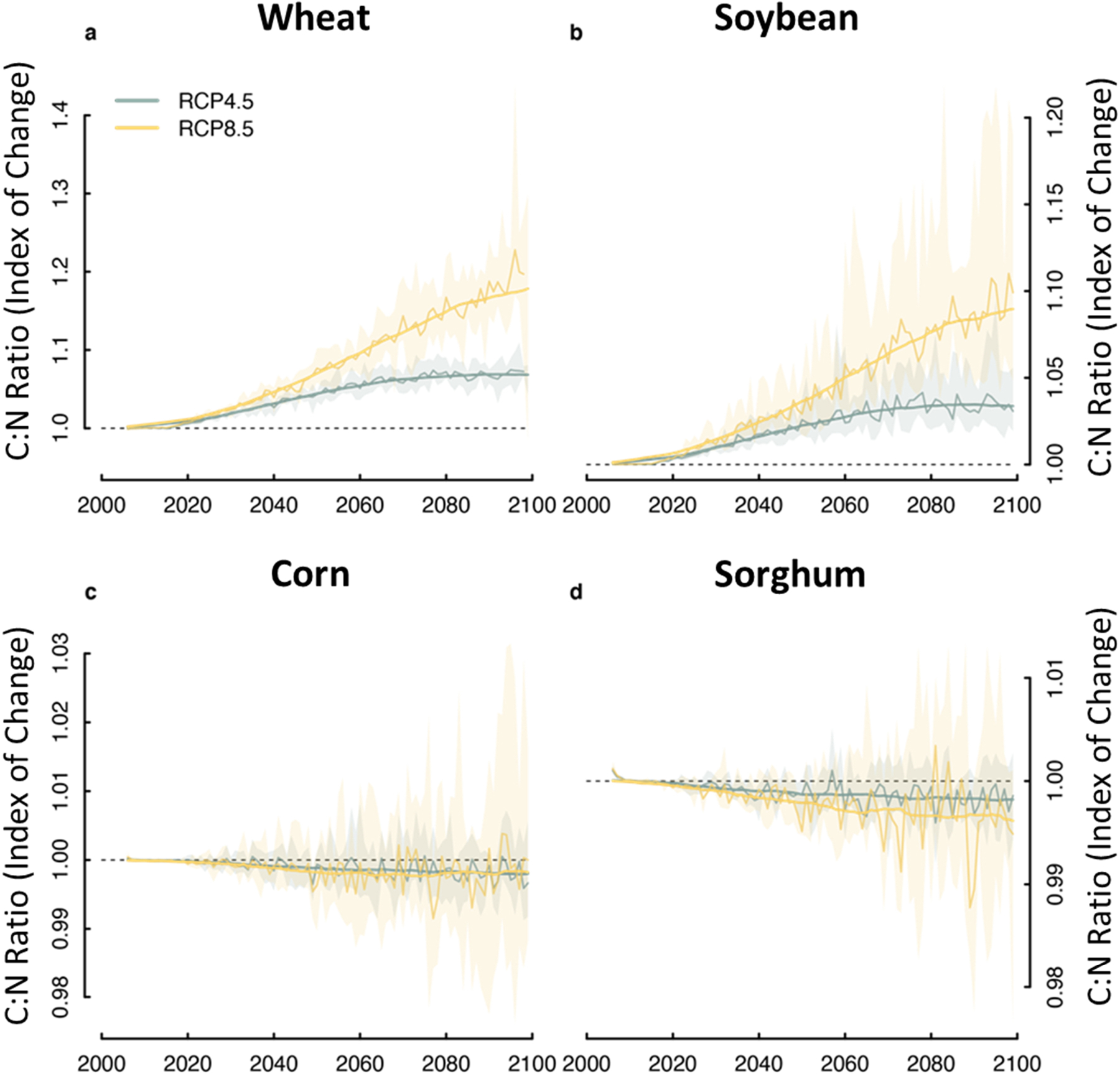
CO₂ effect on nutritional content as shown by the C:N ratio under default (i.e., transient) divided by the C:N ratio under constant 2015 CO₂. Higher C:N ratios can generally be interpreted as lower nutritional quality. Results are from LPJmL driven by LOCA-downscaled outputs from the 6 CMIP5 models used in this study for RCP4.5 and RCP8.5.

3.2. Economic modeling results

Below, we present key results from the economic modeling along with results from some sensitivity experiments on important input parameters (e.g., including/excluding effects of water availability, livestock sensitivity, and international trade demand). We also analyzed the sensitivity to adaptation, pest and disease damages, flood frequency, waterlogging, and surface ozone exposure. The base case climate change runs we used in our economic analyses utilized climate change inputs from the 6 aforementioned GCMs, LPJmL-estimated crop yields for 6 major crops, econometric estimates for 8 additional crops plus the livestock productivity changes, and surface water availability changes.

One of the factors that we examined is total welfare change, which we define as the change in the summed total of domestic consumers’ and producers’ surplus plus surplus associated with a mixture of: a) surplus associated with international region-specific supply and demand curves for corn, soybeans, rice, sorghum, and the wheat types; and b) excess export demand and import supply curves for many other primary and secondary commodities (for example, items like oats, canola, tomatoes, oranges, butter, cheese, and beef). The welfare maximization also gives the optimal solution of market equilibrium in the perfect competition agricultural commodity market as shown in McCarl and Spreen (1980).

3.2.1. Analysis of the basic climate arrival runs

In the economic analyses, we first explored how imposing climate change-altered crop, livestock, and water estimates affected: a) total welfare, b) consumer, producer and international effects, c) price and quantity indices, d) price and quantity amounts for major commodities, e) crop acres for major commodities, and f) shifts in the locus of production. In these experiments we used the LPJmL results for corn, soybeans, spring wheat, winter wheat, sorghum, and grass, and the econometric model for spring barley, rice, corn silage, upland cotton, oats, sugar beets, sugar cane, durum wheat, and livestock.

3.2.1.1. Welfare changes.

In Fig. 7 we portray changes in welfare averaged across the climate models at each warming level: 1) US domestic consumers, 2) US domestic producers, 3) an aggregate of welfare accruing to the sum of international producers and consumers, and 4) the sum of all of these. For perspective on the size of these results, US net farm income, which is the counterpart of domestic producers’ surplus, has varied since 2009 between $61B⁹ and $123B, with $60-$75B being more common in the recent past.

Fig. 7.

Average annual ensemble welfare changes at different arrival degrees under the 2020 base economy (results in billions of 2019 USD).

Our results show the maximum domestic gain is about $16B for producers, along with as much as a $3.2B gain or a $10.6B loss for consumers, and a $6.3B gain for the net international surplus (Fig. 7). Total welfare across all of society exhibits escalating gains to $13.8B at 5 °C, but drops to an $11.7B gain at 6 °C. Domestic consumers’ welfare exhibit gains to $3.2B at 3 °C, followed by a drop as arrival temperatures increase, reaching a loss of $10.6B at 6 °C. The consumers benefit from the increasing crop production and associated reduction in prices, but are affected by losses in livestock products mainly due to reduction in production and increased livestock prices. Over the warming degrees, the loss from livestock is higher than the gain from crops. Domestic producers’ welfare rises to the end of the century at the 6 °C warming level for similar reasons. The crop farmers lose money due to the reduction in prices coupled with the inelastic demand. But the reduction in crop prices also reduces the input cost in the livestock sector, which partially mitigates the effect on livestock product consumers, estimated using the FASOM model based on LPJmL-projected climate impacts and the minor crop econometrics under LOCA-CMIP5 climate scenarios.

3.2.1.2. Price and quantity indices.

Effects of climate change on market prices and quantities produced were computed for a range of commodity index groupings using Fisher ideal index numbers that reflect the average change in price or quantity computed over a basket of goods,¹⁰ much like the commonly reported consumer price index. The quantity covering all farm production, including all primary crop and livestock commodities, increases by 6% from 2019 to the 3-degree level and then declines to just 4% above baseline by the 6-degree level. This reflects a generally positive impact of climate change (particularly CO₂ fertilization) on crop yields and negative impact on livestock products. The price index for all farm production falls from 2019 levels by 4% by 3 °C then rises above 2019 levels by 1% by 6 °C of warming.

Amongst all crops, the results show the largest drop in price for cotton (as much as 48%) due to large increases in cotton supply (as much as 81%), as cotton gains large yield increases from CO₂ fertilization (see discussion in Attavanich and McCarl, 2014). There are smaller decreases in price indices for all farm production, all crops, the grain-soybean complex, and bulk exports. There is an initial decline in the price of crops other than grain and soybeans out to three °C warming, followed by an increase in price at higher warming levels. Corn shows a small production decrease as does durum wheat. Production for the other wheats increases because temperature and CO₂ conditions are projected to become more favorable in northern parts of the country.

To estimate variations in livestock price and quantity, we first estimated changes in production based upon an econometric model estimated over historical USDA data as described in the Methodology section. General production trends include an increase in milk production and calf survival rates and a decrease in feedlot cattle slaughter weight and calving rate. The projected increase in milk production and calf survival rates is most prominent in northern regions where cold stress is reduced as a function of climate change. The resulting changes in livestock price and quantity are relatively small (as much as 4%) excepting for the 6 °C case where the livestock price rises by 11% while production declines 7%. In general, for both crops and livestock there is a negative correlation between price and production quantity, which one would expect in a model with downward sloping demand.

The FASOM results show a decline in harvested acres as temperatures increase for most major crops, except for soybeans and soft white wheat. Corn generally shows only small changes in harvested acres.

3.2.2. Locus of production

We analyzed shifts in production locations by assessing geographic changes in the weighted location centroid of crop production, as shown in Fig. 8.

Fig. 8.

Shifts in ensemble average weighted centroid of crop production by selected crops and arrival degree. Centroids of each crop are indicated by continuum from a light to a darker color as the arrival degrees increase.

The centroids of each crop are marked by continuum from a light to a darker color as the arrival degrees increase, along with the total moving distance from now to 6 arrival degrees. In the figure we see the weighted centroids for most crops are moving to cooler regions (northward and or up in elevation towards the Rocky Mountains) as the arrival degrees increase, except soybeans which move slightly southwest. The results are similar to those estimated in Cho and McCarl (2017), who used an econometric model employing historical U.S. data, and Attavanich and McCarl (2014), who examined the impacts of climate change and CO₂ fertilization. Cotton, whose yield response is not discussed in detail in this paper but is in Attavanich and McCarl (2014), is particularly strongly stimulated by increasing CO₂ levels.

3.3. Sensitivity analyses

In our second analysis we did a sensitivity study regarding the effect of including or excluding a number of items that are certainly relevant to climate effects on agriculture. To gauge the sensitivity, we undertook analyses in which we varied one particular element at a time holding all other elements constant. All of this was done relative to the 2020 economy.

Fig. 9 shows the welfare change associated with each of the factors considered in this set of sensitivity analyses. All welfare effects were derived from FASOM. The factors with negative effects, in approximate descending order of importance, are: adding flood damage; adding international trade effects; replacing the process-based model with the econometric yield model; adding ozone damage; adding waterlogging effects; adding pest and disease damage; and holding surface water availability constant. The factors with positive effects, in approximate descending order of importance, are: adding adaptation and removing livestock sensitivity.

Fig. 9.

Changes in economic welfare associated with each of the sensitivity analyses described in this section.

More information on each of these sensitivity analyses is provided in the subsections below.

3.3.1. International trade implications included

The implications of international trade were assessed including or excluding estimates of climate change impacts on the rest of the world’s production and excess demand, as developed by the International Food Policy Research Institute (IFPRI), 2019; Robinson et al., 2015).¹¹ Adding trade effects decreased ensemble average total welfare by $13.5B under the 3 °C case and by $23.8B under the 6 °C case, compared to the above results. Thus, inclusion of the IFPRI-based trade sensitivity is a large welfare-decreasing factor. It is worth noting that the IFPRI trade sensitivity results span a vastly larger range than do the bilateral trade change assumptions used in the 2000 US National Assessment (Reilly et al., 2002). Given the large difference between the IFPRI-driven results and those from Reilly et al., further study is warranted using a wider variety of contemporary trade sensitivity results.

3.3.2. Econometric yield model projections replaced by those from LPJmL

Replacing LPJmL yields of the 6 simulated commodities (corn, winter wheat, spring wheat, soybean, sorghum, and grassland) with yields from the econometric model had a substantial impact. This substitution of crop models changed the nature of the total welfare results from increases as arrival temperatures increase to results where the welfare initially rises, then reverses direction at 3 °C to become ever increasing losses. In particular, by the 6 °C warming level the use of the econometric yields leads to a decline in overall welfare of $28.1B compared to the LPJmL results where there was an $11.7B total welfare gain. These results reflect the econometric yield modeling conclusions in the above discussion that identify the LPJmL estimates as more positive relative to the regression-based estimates. It is also worth reiterating that both the LPJmL and the econometric yield model results were shown to be more positive than the GGCMI-CMIP6 ensemble median. It would be valuable to extend this work with a larger set of model-based crop yield simulations.

3.3.3. Surface ozone concentration increased

We explored the potential impact of increased surface ozone damages using crop yield reductions based on May-Sept average ozone incidence projections from Nolte et al. (2021) under RCP 8.5 and 4.5. Those ozone changes were fed into a region- and crop-specific ozone dose-yield sensitivity model estimated via regressions developed by Da et al. (2020). The resultant impacts in FASOM of surface ozone in these scenarios are reductions in overall welfare of $3.9B under surface ozone increases projected by Nolte et al. (2021).

3.3.4. Crop adaptation included

Research has shown that adaptation can moderate or even reverse many of the projected negative crop yield changes and can greatly alter total welfare effects (e.g., see discussion in Amatu-Aisabokhae et al., 2012). Crop adaptation actions such as earlier planting dates, altered varieties, crop breeding for more drought and pest resistance, changes in irrigation, and other crop management adaptation measures are not explicitly included in the LPJmL simulations. To generate insight on the importance of crop management adaptations on the economic results of our base simulations, without conducting an extensive set of adaptation scenarios, we conducted a sensitivity experiment in which the yields from LPJmL were modified uniformly using educated assumptions about changes in yield percentage. In the two adaptation scenarios we assumed a 50% reduction in the crop yield sensitivity (indicating that adaptation has moderated yield losses) and either a 5% or 25% enhancement to increases in crop yields (indicating that adaptation has further benefited increasing yields). The 50% reduction was chosen based on Rising and Devineni (2020), while the 5% and 25% enhancement amounts were arbitrarily chosen to test the sensitivity of results to this possibility. We estimate the welfare consequences of the yield enhancements to be + $2.7B and + 5.7B per year for these two scenarios.

3.3.5. Waterlogging damage included

GCM projections indicate that climate change has the potential to increase total precipitation in regions like the Corn Belt (Hayhoe et al., 2018). This would increase the potential for waterlogging of agricultural soils that in turn cause yield reductions (e.g., Arduini et al., 2019, Kaur et al., 2019, Rosenzweig et al., 2002). To develop insight into the magnitude of such an effect we imposed a uniform 5% yield reduction on locations where mean springtime (March-May) precipitation increases by at least 10% in the LOCA dataset (introduced in the scenarios discussion above) in 2050–2059, relative to 1980–2005. The 5% yield reduction is an approximation of the magnitude of yield reductions cited in Kaur et al. (2019). The affected regions are mainly in the US Midwest. The resultant FASOM simulation showed an overall welfare decline of $3.8B per year.

3.3.6. Livestock production climate sensitivity eliminated

Most climate change studies omit the effects of climate change on livestock productivity. To investigate the impacts of including such sensitivity, we ran cases with and without such impacts. In this sensitivity analysis, we added or eliminated climate change effects on beef and dairy cattle calving birth and survival rates, milk production, and the slaughter weight of feedlot fed beef. Eliminating livestock productivity effects increased overall welfare $1.9B under the 3 °C and $4.3B under the 6 °C cases. Thus, including livestock productivity implications leads to about a 20% reduction in welfare gains.

3.3.7. Pest and disease damage included

Pests and diseases damages are expected increase under climate change (Gowda et al., 2018). While there are many efforts to expand models so they directly represent crop losses from pests (Donatelli et al., 2017; Savary et al., 2018; Ziska et al., 2019), definitive results or available scenarios have not conclusively arisen. Given the diversity of U.S. cropping systems and locations and pest incidences (exhibiting specific combinations of pests), there is not a strong basis in our type of analysis for establishing a crop- and region-specific damage scenario. Thus, we assessed a scenario that assumes uniform yield losses of 1% due to pest and disease damage. We find under that scenario that there is a $1.8B decrease in welfare at the 3 °C warming level.

3.3.8. Flooding scenarios

Flooding is another mechanism that can damage crops. Climate models generally indicate an increase in the frequency of flooding (e.g., USGCRP, 2018, Wobus et al., 2017). In this case, the damage is due to the termination of growth due to physical damage from ponded or moving water (vs. the subsurface rotting effect of waterlogging). To assess the sensitivity of the results to flooding we imposed a pattern of impacts on corn, wheat, and soybean yields based on observed damages from the 1993 Midwestern flood. We assumed in constructing the estimate that crops are planted, but then in select years flooding reduces acres harvested and yields in the same percentage amounts as occurred after the 1993 flood. We ran FASOM under normal conditions and locked in the planted acres but then adjusted yield and re-ran to see welfare and market effects. The welfare loss when the 1993 event was imposed within the FASOM framework is $40.6B. Thus, if this is a 1-in-100 year event, its annualized damage is $0.4B per year. If the frequency of a 1993-like flood increases to once every 50, 25, 10, or 5 years in the future (i.e., 2x – 20x increase), the annualized damages would be $0.8B, $1.6B, $4.1B, and $8.1B, respectively.

3.3.9. Surface water availability held constant

The least important of the factors that were examined was the removal of climate change-driven changes in surface water availability (holding it at the constant baseline level for all GCMs), leading to a decrease in overall welfare of up to $0.16B relative to the base case. This small level of sensitivity likely exists for several reasons: a) the water sensitivity was only applied to surface water and in the model results there were shifts to more reliance on groundwater; b) dryland crops could be substituted; c) in many of the main irrigated areas, reliance on groundwater (vs. surface water) is common; d) the model does not cover most fruits and vegetables and thus biases downward the damage estimates; and e) since production was increasing in many cases, there was not much effect of reducing irrigation.

4. Conclusions

This study provides: (1) estimates of changes in U.S. agricultural yields resulting from climate change under CMIP5 projections from both physical and econometric models; (2) economic estimates of resulting changes in prices, economic welfare, and other measures; and (3) economic estimates of how several often-discussed climate-related factors affect the results.

Our yield estimates fall within the range of prior estimates. Our estimates using the process-based LPJmL crop simulation model projects future increases in wheat, grassland, and soybean yield due to climate change with corn and sorghum showing more muted responses likely due to their lesser CO₂ sensitivity. Yields from an econometric model tend to show somewhat less positive effects. Regionally, yields in the south and east tend to decrease or show the smallest increases. The north and northwest tend to show larger increases in yields.

The economic impacts estimated using the LPJmL model yields imposed on the 2020 economy show a maximum gain in economic welfare of $16B to domestic producers by the end of the 21st century, a $6.3B maximum gain for international trade, and a $10.6B maximum loss for domestic consumers, resulting in a total welfare gain of $11.7B relative to a no climate change baseline. Using the LPJmL projections, large price reductions are projected for cotton, soybeans, and wheat. Large production increases are projected for cotton, soybean, wheat, and sorghum. When the yield projections from LPJmL are replaced with those developed using the econometric models, total welfare turns from a gain to a loss of more than $28B. Please refer to Table ESM-2 for a discussion of the relative strengths and weaknesses of process-based and econometric models. As noted in Section 3.2, in this analysis we found it important to assume a constant economy in order to clearly discern the impacts of climate change.

Our sensitivity analyses testing the importance of an array of factors show that the economic results can be significantly altered by their inclusion in a number of cases. The most important factors are those about economic growth, flooding, international trade, and the type of yield model used. Although we did not explicitly assess the relative economic importance of model responses to CO₂ fertilization, uncertainties associated with greenhouse gas emissions scenarios, and the choice of the climate models, the significant impact that these factors have on our crop modeling results suggest that these factors could have major effects on economic welfare. Somewhat less, but not insignificant factors include impacts associated with crop management for adaptation, changes in livestock productivity, and damages from surface ozone concentration, waterlogging, and pests and diseases.

This study points toward several areas that would benefit from additional research and model development. One thing that would be beneficial is to better and more explicitly simulate factors that we addressed in the sensitivity analysis in order to assess interactions between each and to make assessments of their net effect. Another piece of future research that could help to bound uncertainty estimates of the net economic effects would be to repeat key elements of this work using a broader range of yield models whose outputs are fed into an array of economic models.

Data availability

The model outputs will be shared upon request. Portions of the processing code are not publicly available.

References

- Adams DM, Alig RJ, Callaway JM et al. 1996. The Forest and Agricultural Sector Optimization Model (FASOM): Model Structure and Policy Applications. Research Paper PNW-RP-495. U.S. Department of Agriculture, Forest Service. and Steven M. WinnettAinsworth, E.A. and S.P. Long (2021) 30 years of free-air carbon dioxide enrichment (FACE): What have we learned about future crop productivity and its potential for adaptation? Global Change Biology, 27(1). [DOI] [PubMed] [Google Scholar]
- Amatu-Aisabokhae RA, McCarl BA, Zhang YW, 2012. Agricultural Adaptation: Needs, Findings and Effects, Handbook on Climate Change and Agriculture. In: Mendelsohn R, Ariel A (Eds.). Edward Elgar, Northampton,MA, pp. 327–341. [Google Scholar]
- Arduini I, Makie K, Francesca L, 2019. Crop response to waterlogging. Front. Plant Sci. 10, 1578. [DOI] [PMC free article] [PubMed] [Google Scholar]
- Attavanich W, McCarl BA, 2014. How is CO2 affecting yields and technological progress? a statistical analysis. Clim. Change 124 (4), 747–762. [Google Scholar]
- Augustine DJ, Blumenthal DM, Springer TL, LeCain DR, Gunter SA, Derner JD, 2018. Elevated CO2 induces substantial and persistent declines in forage quality irrespective of warming in mixed grass prairie. Ecol. Appl. 28 (3), 721–735. [DOI] [PubMed] [Google Scholar]
- Beach RH, Sulser TB, Crimmins A, et al. , 2019. Combining the effects of increased atmospheric carbon dioxide on protein, iron, and zinc availability and projected climate change on global diets: a modelling study. Lancet Planet Health 3 (7). [DOI] [PMC free article] [PubMed] [Google Scholar]
- von Bloh, Schaphoff W, Müller S, et al. , 2018. Implementing the nitrogen cycle into the dynamic global vegetation, hydrology, and crop growth model LPJmL (version 5.0). Geosci. Model Dev. 11, 2789–2812. [Google Scholar]
- Cheng M, Fei CJ and McCarl BA, 2021. Climate Change Effects on the U.S. Hog production. AAEA Annual Meetings, Austin, TX, August 2021. [Google Scholar]
- Cho SJ, McCarl BA, 2017. Climate change influences on crop mix shifts in the United States. Sci. Rep. 7, 40845. [DOI] [PMC free article] [PubMed] [Google Scholar]
- Daly C, Halbleib M, Smith JI, et al. , 2008. Physiographically-sensitive mapping of temperature and precipitation across the conterminous United States. Int. J. Climatol. 28, 2031–2064. [Google Scholar]
- Donatelli M, Magarey RD, Bregaglio S, et al. , 2017. Modelling the impacts of pests and diseases on agricultural systems. Agric. Syst. 155, 213–224. [DOI] [PMC free article] [PubMed] [Google Scholar]
- Marshall E Aillery M Malcolm S Williams R Climate change, water scarcity, and adaptation in the u.s. fieldcrop sector, ERR-201 U. S. Dep. Agric., Econ. Res. Serv, Novemb. 2015. [Google Scholar]
- Ebi KL, Anderson CL, Hess JJ, et al. , 2021. Nutritional quality of crops in a high CO2 world: an agenda for research and technology development. Environ. Res. Lett. 16 (6), 064045. [Google Scholar]
- EPA 2017a. Multi-Model Framework for Quantitative Sectoral Impacts Analysis: A Technical Report for the Fourth National Climate Assessment. U.S. Environmental Protection Agency, EPA 430-R-17–001. [Google Scholar]
- EPA Climate change impacts on agriculture and food supply U. S. Environ. Prot. Agency; 2017b. [Google Scholar]
- Fatima Z, Ahmed M, Hussain M, et al. , 2020. The fingerprints of climate warming on cereal crops phenology and adaptation options. Sci. Rep. 10 (18013), 2020. 10.1038/s41598-020-74740-3. [DOI] [PMC free article] [PubMed] [Google Scholar]
- Fei C, McCarl BA, 2021. Effect of climate change and research on crop yield growth (Nov 25, 2021). SSRN. 10.2139/ssrn.4066780. [DOI] [Google Scholar]
- Food and Agriculture Organization of the United Nations (FAO), no date: FAOSTAT. http://www.fao.org/faostat/en/#home. [PubMed]
- Frieler K, Lange S, Piontek F, et al. , 2017. Assessing the impacts of 1.5 °C global warming - simulation protocol of the Inter-Sectoral Impact Model Intercomparison Project (ISIMIP2b). Geosci. Model Dev. 10, 4321–4345. [Google Scholar]
- Gowda P, Steiner JL, Olson C et al. 2018. Agriculture and rural communities. In Impacts, Risks, and Adaptation in the United States: Fourth National Climate Assessment, Volume II [Reidmiller DR, Avery CW, Easterling DR et al. (eds.)]. U.S. Global Change Research Program, Washington, DC, USA, 391–437. doi: 10.7930/NCA4.2018.CH10. [DOI] [Google Scholar]
- Hayhoe K, Wuebbles DJ, Easterling DR, et al. 2018. Our Changing Climate. In Impacts, Risks, and Adaptation in the United States: Fourth National Climate Assessment, Volume II [Reidmiller DR, Avery CW, Easterling DR, et al. (eds.)]. U.S. Global Change Research Program, Washington, DC, USA, pp. 72–144. doi: 10.7930/NCA4.2018.CH2. [DOI] [Google Scholar]
- International Food Policy Research Institute IFPRI 2019. IMPACT Projections of Food Production, Consumption, and Net Trade to 2050, With and Without Climate Change: Extended Country-level Results for 2019 GFPR Annex Table 6, IMPACT version 3.3. 10.7910/DVN/WTWRMH, Harvard Dataverse, V2. [DOI] [Google Scholar]
- IPCC 2019. Climate Change and Land: an IPCC special report on climate change, desertification, land degradation, sustainable land management, food security, and greenhouse gas fluxes in terrestrial ecosystems [Shukla PR, Skea J, Calvo Buendia E et al. (eds.)]. [Google Scholar]
- Jägermeyr J, Müller C, Ruane AC, Elliott J, Balkovic J, Castillo O, Rosenzweig C, 2021. Climate impacts on global agriculture emerge earlier in new generation of climate and crop models. Nat. Food. 10.1038/s43016-021-00400-y. [DOI] [PubMed] [Google Scholar]
- Kaur G, Singh G, Motavalli PP, Nelson KA, Orlowski JM, Golden BR, 2019. Impacts and management strategies for crop production in waterlogged or flooded soils: a review. Agron. J. 112 (3), 1475–1501. [Google Scholar]
- Kukal MS, Irmak S, 2018. U.S. agro-climate in 20th century: growing degree days, first and last frost, growing season length, and impacts on crop yields. Sci. Rep. 8, 6977. [DOI] [PMC free article] [PubMed] [Google Scholar]
- Lall U, Johnson T, Colohan P, et al. , 2018. Water. In Impacts, Risks, and Adaptation in the United States: Fourth National Climate Assessment, Volume II [Reidmiller. U. S. Global Change Research Program, Washington, DC, USA, pp. 145–173. 10.7930/NCA4.2018.CH3. [DOI] [Google Scholar]
- von Lampe, Willenbocke M, Ahammad D, et al. , 2013. Why do global long-term scenarios for agriculture differ? an overview of the AgMIP Global Economic Model Intercomparison. Agric. Econ. 45 (1), 3–20. 10.1111/agec.12086. [DOI] [Google Scholar]
- Leakey ADB, 2009. Rising atmospheric carbon dioxide concentration and the future of C4 crops for food and fuel. Proc. R. Soc. B 276, 2333–2343. 10.1098/rspb.2008.1517. [DOI] [PMC free article] [PubMed] [Google Scholar]
- Mbow C, Rosenzweig C, Barioni LG, Benton TG, Herrero M, Krishnapillai M, Liwenga E, Pradhan P, Rivera-Ferre MG, Sapkota T, Tubiello FN, and Xu Y, 2019. Food security. In Climate Change and Land: An IPCC Special Report on Climate Change, Desertification, Land Degradation, Sustainable Land Management, Food Security, and Greenhouse Gas Fluxes in Terrestrial Ecosystems. Shukla PR, Skea J, Calvo Buendia E, Masson-Delmotte V, Portner H-O, Roberts DC, Zhai P, Slade R, Connors ¨S, van Diemen R, Ferrat M, Haughey E, Luz S, Neogi S, Pathak M, Petzold J, Portugal Pereira J, Vyas P, Huntley E, Kissick K, Belkacemi M, and Malley J, Eds., Intergovernmental Panel on Climate Change. [Google Scholar]
- McCarl BA, Spreen TH, 1980. Price endogenous mathematical programming as a tool for sector analysis. Am. J. Agric. Econ. 62 (1), 87–102. [Google Scholar]
- Meinshausen M, Smith SJ, Calvin K, et al. , 2011. The RCP greenhouse gas concentrations and their extensions from 1765 to 2300. Clim. Change 109, 213. [Google Scholar]
- Nolte C, Spero T, Bowden J, et al. , 2021. Regional temperature-ozone relationships across the U.S. under multiple climate and emissions scenarios. J. Air Waste Manag. Assoc. 71 (10), 1251–1264. [DOI] [PMC free article] [PubMed] [Google Scholar]
- Pierce DW, Cayan DR, Thrasher BL, 2014. Statistical downscaling using Localized Constructed Analogs (LOCA). J. Hydrometeorol. volume 15, 2558–2585. [Google Scholar]
- Polley HW, Briske DD, Morgan JA, et al. , 2013. Climate change and North American rangelands: trends, projections, and implications. Rangel. Ecol. Manag. 66 (5), 493–511. [Google Scholar]
- Portman FT, Siebert S, Doll P, 2010. MIRCA2000 - Global monthly irrigated and rainfed crop areas around the year 2000: a new high-resolution data set for agricultural and hydrological modeling. Glob. Biogeochem. Cycles 24 (1). [Google Scholar]
- Beach RH Adams DM Alig RG et al. Model documentation for the forest and agricultural sector optimization model with greenhouse gases (FASOMGHG) Draft Rep. Prep. Sara Bushey Ohrel U. S. Environ. Prot. Agency Clim. Change Div., Wash., DC: 2010. [Google Scholar]
- Reilly JM, Hrubovcak J, Graham J, et al. , 2002. Changing Climate and Changing Agriculture: Report of the Agricultural Sector Assessment Team, U.S. National. Assessment, prepared as part of USGCRP National Assessment of Climate Variability. Cambridge University Press,. [Google Scholar]
- Reilly JM, Tubiello F, McCarl BA, et al. , 2003. US agriculture and climate change: new results. Clim. Change 57, 43–69. [Google Scholar]
- Rising J, Devineni N, 2020. Crop switching reduces agricultural losses from climate change in the United States by half under RCP 8.5. Nat. Commun. 11, 4991. [DOI] [PMC free article] [PubMed] [Google Scholar]
- Robinson S, Mason d′Croz D, Islam S et al. 2015. The International Model for Policy Analysis of Agricultural Commodities and Trade (IMPACT): Model description for version 3. IFPRI Discussion Paper 1483. International Food Policy Research Institute (IFPRI). http://ebrary.ifpri.org/cdm/ref/collection/p15738coll2/id/129825. [Google Scholar]
- Rojas-Downing Melissa, M., Pouyan Nejadhashemi A, Harrigan Timothy, Woznicki Sean A., 2017. Climate change and livestock: Impacts, adaptation, and mitigation. Clim. Risk Manag. 16, 145–163. [Google Scholar]
- Rosenzweig C, Elliott J, Deryng D, et al. , 2014. Assessing agricultural risks of climate change in the 21st century in a global gridded crop model intercomparison. Proc. Nat. Acad. Sci. 111 (9), 3268–3273. [DOI] [PMC free article] [PubMed] [Google Scholar]
- Rosenzweig C, Tubiello FN, Goldberg R, Mills E, Bloomfield J, 2002. Increased crop damage in the US from excess precipitation under climate change. Glob. Environ. Change 12 (3), 197–202. [Google Scholar]
- Savary S, Nelson AD, Djurle A, et al. , 2018. Concepts, approaches, and avenues for modelling crop health and crop losses. Eur. J. Agron. 100, 4–18. [Google Scholar]
- Schaphoff S, von Bloh W, Rammig A, et al. , 2018a. LPJmL4 – a dynamic global vegetation model with managed land – Part 1: model description. Geosci. Model Dev. 11, 1343–1375. [Google Scholar]
- Schaphoff S, Forkel M, Muller C, et al. , 2018b. LPJmL4 – a dynamic global vegetation model with managed land – Part 2: model evaluation. Geosci. Model Dev. 11, 1377–1403. [Google Scholar]
- Schlenker W, Roberts MJ, 2009. Nonlinear temperature effects indicate severe damages to U.S. crop yields under climate change. PNAS 106 (37), 15594–15598. 10.1073/pnas.0906865106. [DOI] [PMC free article] [PubMed] [Google Scholar]
- Toreti A, Deryng D, Tubiello FN, Müller C, 2020. Narrowing uncertainties in the effects of elevated CO2 on crops. Nat. Food 1 (775–782), 2020. [DOI] [PubMed] [Google Scholar]
- USDA, 2020. Agricultural Productivity in the U.S. US Department of Agriculture Economic Research Service. https://www.ers.usda.gov/data-products/agricultural-productivity-in-the-us/ Accessed July 6, 2020. [Google Scholar]
- USGCRP 2018. Climate Science Special Report: Fourth National Climate Assessment, Volume I [Wuebbles DJ, Fahey DW, Hibbard KA et al. (eds.)]. U.S. Global Change Research Program, Washington, DC, USA, 470 pp, doi: 10.7930/J0J964J6. [DOI] [Google Scholar]
- Wang M, 2020. Three essays on economic and environmental analysis of climate change adaptation and mitigation in the U.S. agricultural sector. Tex. AM Univ. [Google Scholar]
- Wobus C, Gutmann E, Jones R, et al. , 2017. Climate change impacts on flood risk and asset damages within mapped 100-year floodplains of the contiguous United States. Nat. Hazards Earth Syst. Sci. 17, 2199–2211. [Google Scholar]
- Fan XX McCarl BA Wu XM et al. A spatial econometric analysis of climate change effects on milk production Draft Pap. Tex. AM J. Submiss. Chapter Thesis Xinxin Fan; 2020. [Google Scholar]
- Da Y McCarl BA Xu Y Effects of ozone and climate on historical (1980–2015) crop yields in the United States: implication and mid-21st century projection of climate change effects Draft Pap. Tex. AM J. Submiss. Draft Chapter Thesis Yabin Da; 2020. [Google Scholar]
- Yu ECH, 2014. Case Studies on The Effects of Climate Change on Water, Livestock and Hurricanes, Ph.D. Dissertation, Texas A&M University. [Google Scholar]
- Yu ECH, McCarl BA, Park SC, 2020. Feedlots, climate change and dust. Draft paper Texas A&M under journal submission and chapter in thesis by Chin-Hsien Yu. [Google Scholar]
- Zhu C, Kobayashi K, Loladze I, et al. , 2018. Carbon dioxide (CO2) levels this century will alter the protein, micronutrients, and vitamin content of rice grains with potential health consequences for the poorest rice-dependent countries. Sci. Adv. 4 (5). [DOI] [PMC free article] [PubMed] [Google Scholar]
- Ziska LH, Blumenthal DM, Franks SJ, 2019. Understanding the nexus of rising CO2, climate change, and evolution in weed biology. Invasive Plant Sci. Manag. 12, 79–88. [Google Scholar]
Associated Data
This section collects any data citations, data availability statements, or supplementary materials included in this article.
Supplementary Materials
Data Availability Statement