RNA fold prediction by Monte Carlo in graph space and the statistical mechanics of tertiary interactions

Abstract

Using a graph representation of RNA structures, we have studied the ensembles of secondary and tertiary graphs of two sets of RNA with Monte Carlo simulations. The first consisted of 91 target ribozyme and riboswitch sequences of moderate lengths (<150 nt) having a variety of secondary, H-type pseudoknots and kissing loop interactions. The second set consisted of 71 more diverse sequences across many RNA families. Using a simple empirical energy model for tertiary interactions and only sequence information for each target as input, the simulations examined how tertiary interactions impact the statistical mechanics of the fold ensembles. The results show that the graphs proliferate enormously when tertiary interactions are possible, producing an entropic driving force for the ensemble to access folds having tertiary structures even though they are overall energetically unfavorable in the energy model. For each of the targets in the two test sets, we assessed the quality of the model and the simulations by examining how well the simulated structures were able to predict the native fold, and compared the results to fold predictions from ViennaRNA. Our model generated good or excellent predictions in a large majority of the targets. Overall, this method was able to produce predictions of comparable quality to Vienna, but it outperformed Vienna for structures with H-type pseudoknots. The results suggest that while tertiary interactions are predicated on real-space contacts, their impacts on the folded structure of RNA can be captured by graph space information for sequences of moderate lengths, using a simple tertiary energy model for the loops, the base pairs, and base stacks.

INTRODUCTION

While RNA fold prediction has a long history, it remains a challenging problem, especially for structures with tertiary interactions. Recent advances in the field have been reviewed by a number of authors (Fallmann et al. 2017; Schroeder 2018; Zhao et al. 2021). The most popular methods that have proven to be successful for predicting secondary structures are based on thermodynamic parameters such as those of Turner et al. (Serra and Turner 1995; Schroeder and Turner 2009; Turner and Mathews 2010) using a dynamic programming algorithm such as that of Zuker (Zuker and Stiegler 1981). Tools such as Mfold/UNAfold (Zuker 2003; Markham and Zuker 2008), ViennaRNA (Hofacker 2003; Lorenz et al. 2011), RNAstructure (Reuter and Mathews 2010) are based on this. More recently, instead of focusing on the lowest energy fold, the ensemble of thermodynamically viable structures has come into focus, and some secondary structure prediction tools based on this have been reviewed by Schroeder (2018). A number of machine learning methods for secondary structure prediction have also been reported (Zhao et al. 2021), and some of them integrate thermodynamic information into their model (Sato et al. 2021).

The connection between secondary structure prediction and graphs was first introduced by Tinoco et al. (1971). The complete topology of RNA secondary structures has been characterized by Waterman et al. (Waterman and Smith 1978, 1986; Penner and Waterman 1993; Schmitt and Waterman 1994). A comprehensive introduction and description of various graphs as used for RNA modeling was provided by Schlick (2018). Cord graphs provide a simple representation of RNA secondary structures. An example is shown in Figure 1A. The circumference represents the nucleotide sequence from the 5′ end to the 3′ end in the clockwise direction. The thin arcs, or the cords, represent base pair contacts. For secondary contacts, these cords do not cross each other. This noncrossing rule is the key defining feature of RNA secondary structures.

FIGURE 1.

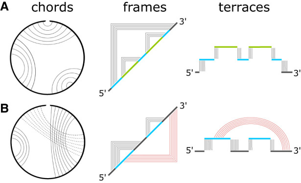
Three types of graphs representing (A) RNA secondary and (B) RNA tertiary structures. In a cord graph, arcs connect bases that are paired. In a frame graph, telescoping picture frames connect paired bases. In a terrace graph, junctions (or loops) are visualized as flat terraces supported on top of pillars representing the two strands that make up the duplex bounding the junction. The terraces on the right are color-coded to match the junction sequences on the frame diagrams in the center. Tertiary contacts are represented by frames on the lower half plane in a frame diagram, and by rainbow arcs in a terrace diagram.

Many topologically equivalent representations can be used. Two of these are shown in Figure 1. In the middle column of Figure 1A is an example of a picture frame graph. In a picture frame graph, the nucleotide sequence goes from the bottom left to the top right in the 5′ to 3′ direction along the diagonal, and the base contacts are represented as points on a square grid on the upper half-plane. A frame graph is similar to the cord diagram described by Waterman. A frame graph can easily be encoded in the form of an adjacency matrix like that introduced by Tinoco et al. (1971), where a 1 on the upper half plane represents a contact between two bases, with the constraint that no more than a single 1 can appear on a column or a row, with the rest of the elements 0. Each frame intersects the diagonal at two nucleotide positions, which are the indices of the two bases that are paired. In secondary structures, none of the frames cross each other. On the adjacency matrix, a duplex appears as a cluster of 1s along the antidiagonal direction, forming the corners of the frames.

A third representation is shown in the right column of Figure 1A, where secondary structures are represented as flat terraces. Each terrace begins with the nucleotide sequence on the 5′ side of a duplex, and it ends with the nucleotide sequence on the complementary strand on the 3′ side of the same duplex. In the example in Figure 1A, these terraces are color-coded to match the bounding duplexes in the frame diagram in the middle column. The blue terrace is bounded by the outermost frame. The two green terraces correspond to the two smaller frames. A terrace diagram makes manifest the loops and junctions in the structure. For example, the blue terrace has three separate sections. Each section is one junction, and the blue terrace represents a three-way junction (3wj). On the other hand, each of the two green terraces has only one section, and they represent one-way junctions (1wj), or hairpin loops. In a terrace diagram, the two nt sequences forming each duplex appear as pillars upon which the terrace is supported. The terrace representation suggests a connection between RNA structures and 1D random walks such as those studied in interfacial problems (Fisher 1984).

All base contacts that are considered tertiary violate the noncrossing requirement of secondary structures, and they produce extraneous diagrammatic elements in the graph representations of RNA structures. Figure 1B shows an example of a pseudoknot, where arcs representing base contacts necessarily cross each other in the cord graph. In the frame diagram, all the violating tertiary contacts are represented by 1s on the lower half plane, and these are shown in red in the middle of Figure 1B. If the red frames were drawn on the upper half plane, they would cross the first black frame on the 5′ side. In a terrace diagram, the only way to represent tertiary contacts is to allow interactions in another dimension outside of the terrace landscape. These are represented by the red rainbow arcs in the right column of Figure 1B. Examples of frame diagrams are shown in Figure 2 for a few structures that contain multijunctions with two (2wj), three (3wj) and four (4wj) loops, as well as several classes of pseudoknots. For H-type pseudoknots and kissing loop interactions, Figure 2D and 2E show that their tertiary interactions on the lower half plane do not cross each other. (Kissing loops are also classified as K-type pseudoknots.) For L-type pseudoknots like the one in Figure 2F, their tertiary interactions have no choice but to cross.

FIGURE 2.

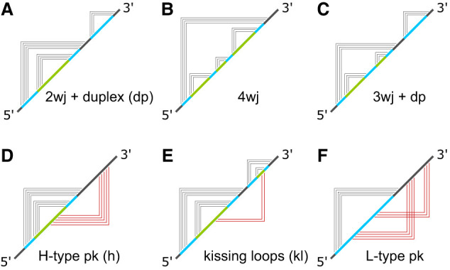
Examples of RNA secondary and tertiary structures and their corresponding frame graphs: (2wj) two-way junction, (3wj) three-way junction, (4wj) four-way junction, (dp) duplex, (pk) pseudoknot, (kl) kissing loop. Panels A–C show secondary graphs. D–F show tertiary graphs.

This paper describes a stochastic strategy for the prediction of secondary and tertiary structures of RNA starting from sequence information alone via a Monte Carlo (MC) simulation exclusively in graph space, essentially implementing a stochastic version of the ideas introduced by Tinoco et al. (1971) and topological studies since Waterman (Waterman and Smith 1978, 1986; Penner and Waterman 1993; Schmitt and Waterman 1994), but supplementing them with tertiary structure prediction capabilities. The applications of graphs to computational RNA structures have been reviewed recently by Schlick and Yan (2023). The RAGTOP method (Kim et al. 2014), which employs a Monte Carlo approach for sampling tertiary conformations of 3D tree graphs using empirical potentials, was applied to riboswitch predictions with pseudoknots (Kim et al. 2015) and then extended to structures with k-turns (Bayrak et al. 2017). Schlick et al. also pioneered computational approaches combined with graphs to study a number of problems in 3D structures, including the prediction of junction topologies (Laing et al. 2012, 2013), performing MC in 3D graph space (Zahran et al. 2015) with empirical potentials (Kim et al. 2015; Bayrak et al. 2017), and assigning general atomic coordinates using fragment assembly (Jain and Schlick 2017; Jain et al. 2018; Meng et al. 2020).

In the following, we describe a stochastic strategy for predicting RNA secondary and tertiary structures via MC simulation in graph space with base pair contacts encoded by an adjacency matrix. An energy function model is used to assign an energy to each graph based on its topological features (loops, junctions, duplexes, tertiary contacts, etc.), and the statistical mechanics of a canonical ensemble of such graphs can then be simulated using straightforward Monte Carlo techniques. Some of the Monte Carlo moves are illustrated in Figure 3 and will be defined in Materials and Methods. On the surface, a method that is based entirely on graph-space information and completely agnostic of real-space information is not expected to do well for predicting tertiary structures, because tertiary contacts are based on interactions that are made in real space when bases pair with each other. Nonetheless, it is worthwhile to find out if there is any graph-space-only energy model for tertiary interactions at all that could produce reasonable tertiary structure predictions without using any real-space information, and if so, what are the contexts within which it would work. Using an MC approach enables us to easily implement and assess any tertiary model without worrying about the algorithmic complexity of how to incorporate that energy function into a folding algorithm. The results show that a simple empirical tertiary energy model works well across a diversity of sequences in predicting tertiary structures for RNA sequences that are shorter than about 150 nt.

FIGURE 3.

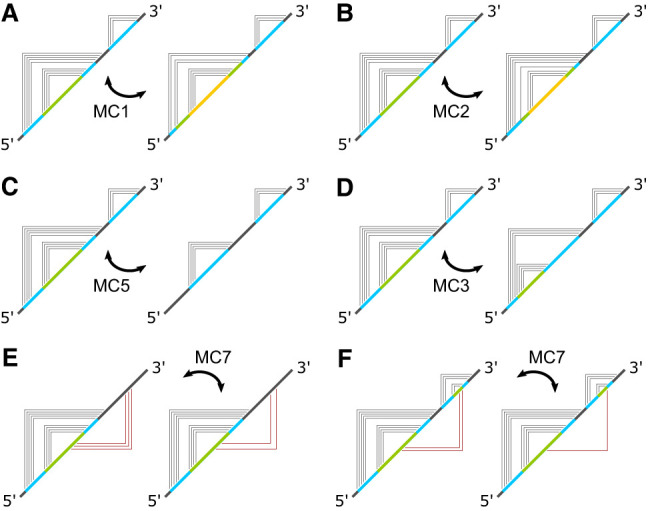
Some of the key MC moves used in the simulation. Panels A–D depict four MC moves that rearrange the secondary structure of a graph. The moves are labeled according to the routines in which they were implemented inside the simulation. Panels (E) and (F) illustrate two MC moves that rearrange the tertiary structure of a graph, both were implemented in the simulation as MC7.

RESULTS AND DISCUSSION

Structures with only secondary interactions

An example of a structure with only secondary interactions in its native fold is shown in Figure 4. 2N3Q (Bonneau et al. 2015) is a 60 nt ribozyme with a 3wj structure. Its nucleotide sequence is given in Figure 4. Figure 4A shows the graph that was the best match for the native structure in the MC-simulated ensemble, and Figure 4B and 4C show the lowest energy graph and the most probable graph in the ensemble. For this sequence, and for the majority of the sequences in Table 3 that are secondary-only, all three are the same graph. The native structure (http://rna.bgsu.edu/rna3dhub/pdb/2N3Q/2d) is provided as a cord graph in Figure 4.

FIGURE 4.

Fold prediction for 2N3Q: (A) best match for native structure, (B) lowest energy and (C) most probable graph in the MC simulated ensemble. (D) Spectrum of the ensemble at μ = 9.99 k_BT, with the most probable graph in pink and a linear fit to the bottom of the spectrum as the orange dashed line. The sequence and the cord graph of the native fold (http://rna.bgsu.edu/rna3dhub/pdb/2N3Q/2d) are given on the lower right. Quality scores for the most probable fold are TPR = 0.91 and mFPR = 0.05.

TABLE 3.

List of targets in the Rzs test set with only secondary interactions in their native structures, giving PDB code and sequence length of each in parentheses

Rzs secondary test set
1KXK (70)	1U9S (161)	2KXM (27)	2LU0 (49)	2MI0 (22)
2MIS (26)	2MTJ (47)	2N3Q (62)	2N3R (62)	2OEU (66)
2OIU (71)	2QUS (69)	2R8S (159)	359D (44)	3BBM (67)
3D2V (77)	3E5C (53)	3F2X (112)	3GS5 (64)	3OXE (88)
3PDR (161)	4GXY (172)	4R4V (186)	4RUM (92)	4Y1M (107)
4YAZ (84)	5DH6 (68)	5LYS (57)	5NDH (16)	5T83 (89)
5U3G (85)	5U6Z (68)	5UZ6 (32)	6AZ4 (42)	6C27 (47)
6CB3 (101)	6CK5 (117)	6EZ0 (27)	6HC5 (18)	6JQ5 (163)
6N2V (99)	7EAG (41)	7ELQ (45)	7MLW (128)	7Q80 (68)
7TZS (80)

Mean quality scores of fold predictions
Model	TPR	mFPR
Vienna	0.731	0.260
ASMC	0.719	0.245

The quality of the fold predictions by ViennaRNA and by ASMC were measured by the true positive rate (TPR), the number of predicted contacts that match native as a fraction of all native contacts, by the modified false positive rate (mFPR), and the number of overpredicted contacts as a fraction of all predicted contacts. Table shows the mean TPR and mFPR scores for Vienna and ASMC for this set. Details are given in Supplemental Table S-01.

In Figure 4A–C, the native contacts are marked by red dots. These native contacts are shown on both the upper and lower half planes. If a secondary contact in the predicted structure matches a native contact, it is reflected by a red dot on the upper left corner of the frame. On the other hand, if a tertiary contact matches a native contact, it will be reflected by a red dot on the lower right corner of a frame on the lower half plane. A match either shows on the upper half plane or the lower half plane, but never both. Every predicted duplex appears as a sequence of telescoping frames with corners moving in the antidiagonal direction. The graphs show that the predicted structure is close to a perfect match, except for one base pair on the outermost hairpin of the 3wj.

Figure 4D shows the distribution, or the spectrum, of the graphs in the simulated ensemble with μ = 9.99 k_BT, where all tertiary contacts had been suppressed. The most probable graph, shown in pink, was also the lowest energy graph. For ensembles with secondary structures only, their spectra typically follow a simple progression like that in Figure 4D. Since the probability of each microstate in the canonical ensemble is proportional to $\exp \left(-E_g/k_{B}T\right)$, the spectrum falls on a straight line with slope −1/k_BT, shown by the orange dotted line in Figure 4D, when plotted on a semilog scale.

The predictions for all 46 secondary-only targets listed in Table 3 are provided in the Supplemental Material. For each target, the most probable structure at the lowest value of μ where the ensemble could be confidently equilibrated was taken as the predicted structure.

To assess the quality of the fold predictions made by ASMC across the 46 target in the Rzs test set with secondary-only folds, Supplemental Table S-01 shows the number of contacts predicted by ViennaRNA and how many of those match the native structure in columns 4 and 5, respectively, and for ASMC in columns 6 and 7. Since each target has a different sequence length, we normalized each of these by the number of contacts, to arrive at a quality score represented by a fraction between 0 and 1. The columns in Supplemental Table S-01 labeled TPR are the true positive rates, which represent the number of predicted contacts that match native as a fraction of all native contacts in each target, for Vienna and ASMC separately. Also known as the “sensitivity” (Reidys et al. 2011), TPR is a goodness score that measures the predictive ability of the model. The columns labeled mFPR in Supplemental Table S-01 represent the modified false positive rate, which is the number of overpredicted contacts as a fraction of all predicted contacts, for Vienna and ASMC separately. mFPR is related to the positive predictive value (PPV) (Reidys et al. 2011) by mFPR = 1 – PPV and represents a badness score that measures the propensity of the model for making overaggressive predictions. (Note that mFPR is not the same as the false positive rate defined in conventional binary classification problems, because true negatives are ill-defined for pairing problems.) For any prediction, a higher value for TPR and a lower value for mFPR reflect better agreement between the predicted fold and the native fold. The averages of these quality scores over the entire test set are shown at the end of Table 3, and the scores for each individual target are given in Supplemental Table S-01. For the six examples illustrated in Figure 5, the quality scores of each prediction are also provided with each graph. Since they have different denominators, TPR and mFPR do not necessarily add up to 1 for each target.

FIGURE 5.

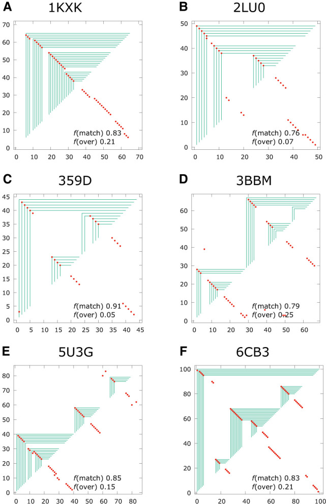
Panels A–F show examples of fold predictions for sequences with only secondary interactions in their native structures.

Suppplemental Table S-01 shows that for a number of the targets in the Rzs test set with only secondary structures, ASMC and Vienna have almost identical mean quality scores. In fact, ASMC and Vienna produced the same fold predictions for 14 of the 46 targets. For most of the rest, ASMC and Vienna produced very similar folds. However, there are also a handful of targets where Vienna and ASMC predicted very different folds, for example, 2N3Q. The mean value of the match quality score, TPR, and the overprediction quality score, mFPR, across the entire sample are given for Vienna and ASMC in Table 3. The mean matched score TPR is 0.731 for Vienna and 0.719 for ASMC, and the mean overprediction score mFPR is 0.260 for Vienna and 0.245 for ASMC. These values suggest that the two models perform with comparable quality for this set of targets with secondary-only structures. For a particular fold prediction, quality scores of TPR > 0.75 in combination with mFPR < 0.25 represent an excellent match against the native structure, and among this set of 46 targets, 23 in Vienna and 18 in ASMC yielded excellent predictions. 2N3Q in Figure 4 and the six examples in Figure 5 illustrate some of these.

Structures with kissing loop interactions

An example of a structure with kissing loop interactions in its native fold is shown in Figure 6. 1Y26 (Serganov et al. 2004) is a 71 nt adenine riboswitch. The overall secondary structure is a 3wj, with a 2 bp kissing loop interaction between the two hairpins. A purine ligand can be sequestered by the loops in this 3wj structure, but the kissing loop interactions are distal from the purine binding site. Figure 6A–C show the best match, lowest energy, and most probable graphs in the ensemble, respectively, for μ = 0.0 k_BT. The most probable graph is also the best match, but the native fold is no longer the lowest energy graph. The spectrum of the ensemble is shown in Figure 6E, showing that the most probable graph is ∼4.5 kcal/mol from the lowest energy state.

FIGURE 6.

Fold prediction for 1Y26: (A) best match for native structure, (B) lowest energy and (C) most probable graph in the MC simulated ensemble. (D) Energy of graphs sampled during a simulation with 0.12 billion MC passes. (E) Spectrum of the ensemble at μ = 0.0 k_BT. (F– H) Three sample structures corresponding to the energies indicated by the orange lines in the spectrum. (I) The ensemble average energy (black dots) of the simulations, the square root of the energy variance from the mean (dashed line above and dashed line below the average) and the entire span of the spectrum indicated by the vertical lines, as a function of μ in units of k_BT. The sequence and the cord graph of the native fold (http://rna.bgsu.edu/rna3dhub/pdb/1Y26/2d) are given on the lower right. Quality scores for the most probable fold are TPR = 0.92 and mFPR = 0.04.

Compared to structures that have only secondary contacts, such as 2N3Q in Figure 4D, the spectrum of 1Y26 in Figure 6E is much more congested. This is due to the proliferation of graphs made possible by the tertiary contacts, which engender a large diversity of graphs that were absent in secondary-only structures. The spectrum of 1Y26 in Figure 6E appears to have two broad humps, one centered at energy ∼ +4 kcal/mol, and the other at ∼−10 kcal/mol. In addition to the most probable and lowest energy graphs, whose energies are shown by the purple and blue lines in the spectrum, respectively, three additional examples are shown in Figure 6F and 6G with their energies in orange, corresponding to the three orange lines in the spectrum. These graphs have various degrees of secondary and tertiary structures in them, some matching native contacts and others not. While the states in the spectrum appear to fall into two humps, the graphs in each group are not obviously related by structure. For example, the most probable graph in Figure 6C and that in Figure 6F appear to belong to the same hump, but their graphs show no relationship with each other except for the outermost helix common to both of them. Similarly, the graphs in Figure 6G and 6H both fall within the high-energy hump in the spectrum, but their structures have little correlation with each other. Figure 6I illustrates the span of the energy spectrum in the ensemble as a function of the prevalence of tertiary contacts according to μ. The top and bottom of the energy spectrum in each ensemble are shown as the vertical lines above and below the average energy of the ensemble in the black circles. As more tertiary contacts are allowed (from right to left in Fig. 6I with decreasing μ), the spectrum expands, encompassing many more graphs, and the ensemble average energy, roughly at the center-of-mass of the spectrum, moves higher at the same time. The square root of the variance of the spectrum is shown by the dashed line and the dotted line above and below the average energy. Figure 6D shows the energy of the graphs sampled by the simulation during a run with 0.12 billion MC passes, showing a cluster of graphs around $\sim +4$ kcal/mol and another around ∼−10 kcal/mol.

The predictions for all 18 targets with kissing loop interactions listed in Table 4 are provided in Supplemental Table S-02. A few examples of the quality of the predictions are also shown in Figure 7. Overall, the kissing loop interactions are predicted correctly for about half of the targets. The typical kissing loop motif involves only a few base pairs, and the model misses some of these, especially those with only two base pairs. Nonetheless, the overall structures of these are largely defined by their secondary contacts, and the kissing loop interactions produce a small perturbation on their overall folds. The simulations correctly predicted a majority of the secondary structures in these targets.

TABLE 4.

Targets in the Rzs test set with kissing loop interactions in their native structures

Rzs kissing loop test set
1Y26 (71)	3D0U (161)	3DIL (174)	3IVN (70)	3LA5 (71)
3RKF (67)	3SKI (68)	4FEN (67)	4FRG (84)	4MGN (164)
4XNR (71)	5C45 (113)	5FJC (95)	5NDI (43)	5SWD (71)
6DN2 (112)	6E1S (33)	6VMY (148)

Mean quality scores of fold predictions
Model	TPR	mFPR
Vienna	0.650	0.269
ASMC	0.707	0.223

See Table 3 for definitions of each data column. Details are given in Supplemental Table S-02.

FIGURE 7.

Panels A–F show examples of fold predictions for sequences with only kissing loops interaction in their native structures.

The quality scores TPR and mFPR are shown for each of the examples in Figure 7. With TPR > 0.75 and mFPR < 0.25, 3D0U and 5NDI are considered excellent matches. Because kissing loop interactions would have shown up in a frame graph as blue frames, notice that the fold predicted by ASMC for 5NDI is missing the 2 bp kissing loop interaction. On the other hand, even though 5FJC and 5SWD missed the mark for being considered excellent, their predicted fold did capture some of the key kissing loop interactions. 5C45 is an interesting example because the predicted fold has poor quality scores with TPR = 0.12 and mFPR = 0.87, but the global structure of the predicted fold is quite reflective of the native fold.

The overall quality of the fold predictions by ASMC compared to Vienna across the 18 targets with isolated kissing loops interactions in the Rzs test set are shown in Supplemental Table S-02. Out of these 18 targets, nine predictions from Vienna produced excellent matches against their native structures, with TPR > 0.75 and mFPR < 0.25, while 11 predictions from ASMC were excellent. As shown in Table 4, the mean match quality score TPR is 0.650 for Vienna and 0.707 for ASMC, while the mean overprediction quality score mFPR is 0.269 for Vienna and 0.223 for ASMC. Based on these scores, ASMC appears to perform slightly better than Vienna, but the limited size of this sample also makes this conclusion somewhat uncertain.

Structures with H-type pseudoknot interactions

An example of a structure with H-type pseudoknot interactions in its native fold is shown in Figure 8. 2MIY (Kang et al. 2014) is a 58 nt class II preQ₁ riboswitch. The folded structure of this molecule contains two hairpin loops, with a tertiary interaction platform between the first loop and the open strand on the distal 3′ end of the sequence. Figure 8A–C shows the best, lowest, and most probable graphs in the μ = 0.2 k_BT ensemble simulated by MC. A predicted contact that matches the native structure shows either as a red dot on the corner of a green frame on the upper half plane of Figure 8C if it is a secondary interaction, or as a red dot on the corner of a blue frame on the lower half plane if it is tertiary. Again, the most probable graph was taken as the predicted structure, which is almost a perfect match to the native fold except for one base pair in the tertiary contacts. Figure 8D shows the energies of the graphs visited by the MC simulation, and the corresponding spectrum is shown in Figure 8E. In this case, the most probable graph, highlighted in pink, was in the middle of the spectrum, far from the lowest energy graph highlighted in blue. Figure 8F illustrates how the spread of the energies in the spectrum, the average energy, and the square root of its variance in the simulated ensemble evolve with the prevalence of tertiary contacts as a function of μ.

FIGURE 8.

Fold prediction for 2MIY: (A) best match for native structure, (B) lowest energy and (C) most probable graph in the MC simulated ensemble. (D) Energy of graphs sampled during a simulation with 0.24 billion MC passes. (E) Spectrum of the ensemble at μ = 0.1 k_BT, with the most probable graph in pink and the lowest energy graph in blue. (F) The ensemble average energy (black dots) of the simulations, the square root of the energy variance from the mean (dashed line above and dashed line below the average) and the entire span of the spectrum indicated by the vertical lines, as a function of μ in units of k_BT. The sequence and the cord graph of the native fold (http://rna.bgsu.edu/rna3dhub/pdb/2MIY/2d) are given on the lower right. Quality scores for the most probable fold are TPR = 0.95 and mFPR = 0.

As for all the targets, the most probable state in Figure 8C was taken as the predicted fold for 2MIY. This graph also happened to be the state in the simulated ensemble that was the best match against the native structure, but no information from the native structure was used to call the predicted fold. The ensemble at μ = 0.2 k_BT was used because Figure 8F shows an unexpected discontinuity in the energy below μ = 0.2 k_BT, indicating potential ergodicity issues with ensembles for μ < 0.2 k_BT. The MC energy trace in Figure 8D suggests that after a short initial equilibration period, the simulated ensemble at μ = 0.2 k_BT seemed to be able to encompass all the energies spanned by the spectrum in Figure 8E.

The predictions for all 27 targets with H-type pseudoknot interactions listed in Table 5 are provided in Supplemental Table S-03. A few examples of the quality of the predictions are also shown in Figure 9. A predicted contact that matches the native structure shows as a red dot on the corner of a green frame on the upper half plane if it is a secondary interaction, or as a red dot on the corner of a blue frame on the lower half plane if it is tertiary, but not both. Overall, the energy model for the tertiary interactions, despite its simplicity, worked well.

TABLE 5.

Targets in the Rzs test set with H-type pseudoknot interactions in their native structures

Rzs pseudoknot test set
2MIY (59)	2QWY (52)	2Z75 (143)	3K1V (34)	3NPQ (54)
3Q3Z (77)	4ENC (52)	4FRN (102)	4JF2 (77)	4KQY (119)
4LVW (89)	4OJI (54)	4OQU (97)	4QJD (71)	4QK9 (124)
4QLM (110)	4RGE (59)	5BTP (75)	5D5L (77)	5KH8 (47)
5NWQ (41)	6FZ0 (49)	6HAG (43)	6N5P (127)	6QN3 (100)
6XKO (96)	6YL5 (35)

Mean quality scores of fold predictions
Model	TPR	mFPR
Vienna	0.651	0.357
ASMC	0.743	0.199

See Table 3 for definitions of each data column. Details are given in Supplemental Table S-03.

FIGURE 9.

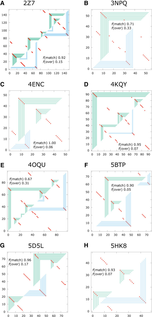
Panels A–G show examples of fold predictions for sequences with H-type pseudoknot interaction in their native structures.

The quality scores TPR and mFPR are shown for each of the illustrations in Figure 9. Using the criteria that TPR > 0.75 and mFPR < 0.25 represents an excellent match, 2Z75, 4ENC, 4KQY, 5BTP, 5D5L, and 5HK8 are considered excellent. 4ENC has a perfect TPR score of 1.0, and as has been emphasized in the last paragraph, some of the predicted contacts match on the upper half plane indicated by the green frames, while the rest match on the lower half plane indicated by the blue frames. A frame intersecting any of the red dots on either the upper or lower half plane is a match for a native contact, and the matches appear either on the upper half plane or the lower half plane, but never both. The examples in Figure 9 all illustrate predictions where the key tertiary interactions were correctly predicted.

The overall quality of the fold predictions produced by ASMC compared to Vienna across the 27 targets with H-type pseudoknots in the Rzs test set are shown in Supplemental Table S-03. Out of these 27 targets, only eight predictions from Vienna produced excellent matches against their native structures with TPR > 0.75 and mFPR < 0.25, while 12 predictions from ASMC were excellent. As shown in Table 5, the mean matched quality score TPR is 0.650 (±0.295) for Vienna and 0.707 (±0.198) for ASMC, while the mean overprediction quality score mFPR is 0.269 (±0.271) for Vienna and 0.223 (±0.176) for ASMC. Based on these metrics, ASMC appears to perform better than Vienna for the targets in Table 5 with H-type pseudoknot interactions.

Overall quality of ASMC fold predictions

In addition to the three sets of targets in the Rzs test sets described above, the Rfam test set in Table 6 represents a more diverse sample of nonhomologous RNA structures. The overall quality of the fold predictions by ASMC compared to Vienna across the 71 targets in the Rfam test set are shown in Supplemental Table S-04. Out of these 71 targets, 40 predictions from Vienna produced excellent matches against their native structures with TPR > 0.75 and mFPR < 0.25, whereas 34 predictions from ASMC were excellent. As Table 6 shows, the mean match quality score TPR is 0.702 for Vienna and 0.713 for ASMC, while the mean overprediction quality score mFPR is 0.225 for Vienna and 0.187 for ASMC. These scores suggest that ASMC appears to perform with comparable quality to Vienna within the more diverse Rfam test set.

TABLE 6.

Targets in the Rfam test set

Rfam test set
1KXK (70)	1M5K (113)	1N8X (36)	1NBS (150)	1P6V (24)
1U9S (161)	1XJR (47)	1Z2J (45)	2KE6 (48)	2L1F (131)
2L3J (71)	2LC8 (56)	2MF0 (72)	2MIY (59)	2N1Q (155)
2NBX (108)	2QUS (69)	2V3C (96)	2Z75 (143)	3D2V (77)
3DIL (174)	3F2X (112)	3NDB (136)	3OXE (88)	3PDR (161)
3Q3Z (77)	3SN2 (29)	3SNP (29)	4FEN (67)	4FRG (84)
4LVW (89)	4OQU (97)	4PQV (68)	4QLM (110)	4RUM (92)
4V2S (57)	4WFL (107)	4YAZ (84)	5BTP (75)	5FJC (95)
5KH8 (47)	5LYS (57)	5NWQ (41)	5T5A (62)	5T83 (89)
6B19 (38)	6CC1 (93)	6CU1 (80)	6FZ0 (49)	6HAG (43)
6JQ5 (163)	6LXD (72)	6MWN (92)	6OL3 (111)	6QN3 (100)
6V5C (66)	6VMY (148)	6WLQ (119)	6XKO (96)	7D81 (50)
7ELP (45)	7JJU (102)	7KGA (90)	7LYF (139)	7QR3 (69)
7SAM (169)	7WIB (50)	8DP3 (90)	8FCS (71)	8GZP (68)
8SH5 (88)

Mean quality scores of fold predictions
Model	TPR	mFPR
Vienna	0.702	0.225
ASMC	0.713	0.187

See Table 3 for definitions of each data column. Details are given in Supplemental Table S-04.

The quality scores of every target in both the Rfam and Rzs test sets are visualized in Figure 10 for ASMC on the top panel, and for Vienna in the bottom panel. For each target, mFPR on the vertical axis (higher is better) is plotted against TPR on the horizontal axis (toward the right is better) for Rfam targets in solid orange and Rzs targets in open circles. The gray area represents the region inside which a particular prediction is considered excellent. Figure 7 suggests that the quality of predictions by ASMC and Vienna are largely comparable, as the mean quality scores in Tables 3, 4, and 6 indicate, while ASMC seems to outperform Vienna for structures with H-type pseudoknots as the mean quality scores in Table 5 suggest.

FIGURE 10.

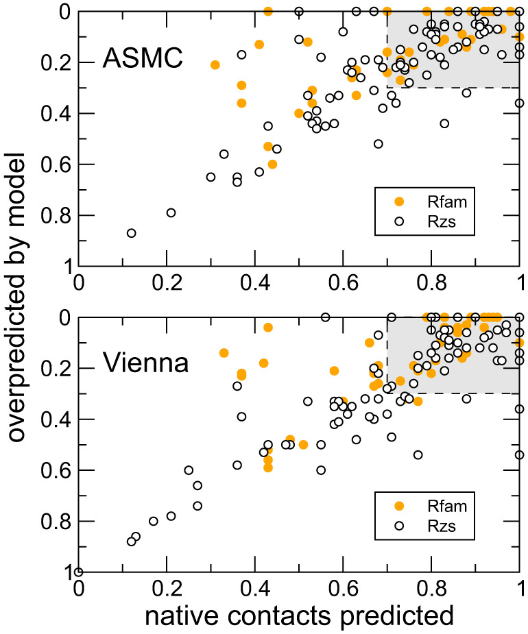
Quality scores of each target are plotted with mFPR on the vertical axis (higher is better) and TPR on the horizontal axis (toward the right is better) for all Rfam targets in solid orange and all Rzs targets in open circles. ASMC predictions are shown in the top panel, and Vienna on the bottom. The gray area represents the region inside which a particular prediction is considered excellent.

Statistical mechanics of tertiary interactions

For an RNA sequence of length N, the maximum number of base pair contacts is N/2. If there are P base pair contacts, the number of possible graphs can be shown to be [N!/(N − 2P)!]/(2^PP!). Taking a 10 nt sequence as an example, the number of graphs with 0, 1, 2, 3, 4, and 5 contacts correspond to 1, 45, 630, 3150, 4725, and 945. Clearly, graphs proliferate with the number of contacts, but the noncrossing constraint of secondary interactions limits them to only a small subset. Base-pairing and favorable stacking in canonically paired duplexes reduce the number of viable secondary graphs further.

To count tertiary graphs, one can start with a secondary frame graph and consider the number of additional graphs that can be constructed by adding tertiary contacts to the lower half plane. The same formula above applies. If there are T tertiary contacts and there are M bases on the open strands in the secondary graph, the number of possible tertiary graphs is [M!/(M − 2T)!]/(2^TT!). Tertiary contacts engender a large number of new graphs. Figure 11 illustrates this for 2MIY. As the value of μ was lowered in the simulation, tertiary contacts were more readily formed. The number of graphs grew, and the spectra became more broad and much more congested at the same time. At μ = 9.99 k_BT in Figure 11A, tertiary contacts were suppressed, and the spectrum followed a straight line with slope −1/k_BT on a semilog scale, like that for 2N3Q in Figure 4D when only secondary graphs were present in the ensemble. The most probable graph, which was also the lowest energy graph at μ = 9.99 k_BT is shown on the right in Figure 11 and highlighted in pink in the spectrum. When tertiary contacts became more prevalent as μ was lowered to 2.00 k_BT in Figure 11B, the most probable graph shifted to higher energy because the center-of-mass of the spectrum moved to the right as the number of graphs proliferates. The spectrum suggests that the graphs fall into two branches, with each one following a straight line with slope −1/k_BT indicated by the two orange dashed lines in Figure 11B. When μ was further lowered to 1.00 k_BT in Figure 11C, more branches developed as the orange dashed lines indicate. The origin of each branch is labeled 0, 1, 2, etc. When μ was lowered to 0.50 k_BT, Figure 11D shows that more branches continued to develop. Each of these branches corresponds to a different number of base contacts in the tertiary structure. The lowest branch has no tertiary contact. The next branch in Figure 11D, whose origin is also the most probable graph in the ensemble, has one tertiary contact. The origin of each branch is labeled by the number of tertiary contacts in blue. When μ was lowered to 0.30 k_BT, even more branches developed and the most probable graph fell inside the branch with five tertiary contacts, revealed by the five blue frames on the lower half plane in its frame graph representation. At μ = 0.30 k_BT, the most probable graph was close to a perfect match to the native fold, but with an energy almost 9 kcal/mol above the lowest energy state according to the empirical tertiary energy function used in the model. Notice that as μ decreases, the branches are closer together because each base that is involved in a tertiary contact picks up an energy penalty equals to μ. If μ is decreased further, the branches will be packed closer together. At some point, their ordering will also begin to reverse.

FIGURE 11.

Panels A–E show evolution of the spectrum of the simulated ensemble for 2MIY as a function of μ in units of k_BT. The most probable graph in each is shown in pink, and its frame graph on the right. (F) Entropy of the ensemble in units of k_B as a function of the chemical potential. The nonmonotonic behavior indicated by the white circles suggests possible sampling ergodicity issues. The dashed line is a guide to the eye.

With the parameters in this empirical tertiary energy model, duplexes formed via tertiary contacts are energetically unfavored. In general, the formation of pseudoknots is known to be energetically costly (Xia et al. 1998; Turner 2000; Cao and Chen 2006, 2009; Bisaria et al. 2017), but a complete energy function for every type of tertiary contacts is not yet available. In lieu of a precise tertiary energy function, the empirical function used in the model produces an uphill energy penalty ∼0.5–1.5 kcal/mol for every doublet base pair when μ is set to 0. Entropic forces resulting from the proliferation of the tertiary graphs make these high-energy graphs possible. If tertiary contacts were not energetically unfavorable, the graph ensembles, even for those structures that do not have tertiary contacts in their native fold, would all have been dominated by tertiary graphs.

While the results suggest that it is the entropic driving force arising from the proliferation of tertiary graphs that enables the ensemble to access higher energy folds, another factor in the simulations may also play a role. MC moves have varying sampling efficiencies, and some are less ergodic than others. In a MC run, the sampling may therefore be attracted to those states out of which moves are very weakly ergodic. This kinetic effect may also lead to a clustering of the microstates similar to that observed in Figure 11. The statistical mechanics of the simulated ensembles of these is similar to those in a glassy system (Mauro and Smedskjaer 2014). Extensive long MC runs (up to 0.4 billion passes) were used to avoid this issue, but there were indeed targets that could not be fully equilibrated. The lowest value of μ at which the ensemble could be reliably equilibrated for each target is listed in Supplemental Tables S-01 to S-04 in the last column. Quite possibly, both the entropic driving force caused by the proliferation of the tertiary graphs as well as the glassiness of the system produced by the kinetics of weakly ergodic sampling are working together to generate the unusual statistical mechanical properties observed in these simulated graph ensembles.

Why does a barebone empirical energy model work for predicting tertiary interactions?

The results in this paper show that a barebone empirical tertiary energy model can indeed perform satisfactorily in predicting tertiary structures of many short RNA sequences up to about 150 nt. As the results show, accounting for the entropic effect of tertiary interactions is the first essential prerequisite for any tertiary energy model. Tertiary interactions lead to a proliferation in the number of graphs in the ensemble on top of secondary-only graphs, and the initiations of tertiary contacts are driven by the enormous diversity of tertiary graphs. The size of the ensemble may be deduced from the scaling properties of the partition function (Flajolet and Sedgewick 2009), but this is sequence-specific and better suited for long homogeneous repeats (Mak and Phan 2021). For sequence lengths like those considered in this study, a more direct approach is to numerically estimate the entropy S of the ensemble of each target as a function of the chemical potential μ from the spectrum using Gibb's formula $S=-k_B{\sum }_g{P}_g\ln P_g$, where the sum is over all graphs generated in the simulated ensemble and P_g is the normalized probability of each graph. S measures the information content in the ensemble. (Notice that this S corresponds only to the entropy of the graph ensemble. Contributions from atomic- and molecular-level motions, conformational variances in the sugar-phosphate backbone, solvent–solute interactions, etc. are not included in S, which is not equal to the full thermodynamic entropy of the corresponding RNA in solution.) For example, an ensemble with entropy S would have the same information content as another ensemble with $N=e^{S/k_B}$ equally probable states. From the spectra of 2MIY in Figures 8E and 11A–E at different values of the chemical potential μ, the estimated entropies are shown in Figure 11F. At large values of μ, tertiary structures were suppressed, and the entropy was low, reflecting a small ensemble. For example, at μ = 2 k_BT, the entropy for the ensemble S/k_B = 1.463, which contains the same information as an ensemble with 4.3 equally probable states. But as μ is lowered, tertiary graphs grew in, resulting in an increase in the entropy, which is expected to grow monotonically with decreasing μ. For example, at μ = 0.2 k_BT, S/k_B = 5.316, and this ensemble contains the same information as another one with 204 equally probable states. The entropy calculated this way, however, is only an estimate of the ensemble entropy, because a finite-length simulation may not generate every possible graph in the ensemble, and the estimated entropy is thus a lower bound to the true ensemble entropy. Illustrating this are the two white circles in Figure 11F for μ = 0 and 0.1 k_BT. As discussed earlier, the discontinuity in Figure 6I at μ < 0.2 k_BT suggests that the sampling for μ = 0 and 0.1 k_BT for 2MIY might have been affected by ergodicity issues, and the entropy versus μ plot in Figure 11F demonstrates this more clearly. Nonmonotonic behavior in S as a function of μ signals potential sampling problems, and it can be used as an additional diagnostic to help determine what is the lowest value of μ that should be used for calling the predicted fold for each sequence.

In the empirical model used here, the energy terms are divided into loops, base pairs and base stacking terms and empirical functions and parameters were assigned to them based on reasonable expectations coming from the same features in the secondary structure energy function. These energy terms, however, are not all independent. For example, the stacking term and the loop energy term add to produce the overall energy cost between every base and its neighbor on each strand inside a duplex, and a multiplicity of loop and stacking energy parameter combinations in the model may generate the same or similar energy for that duplex. There are, in general, large degeneracies in the space of the tertiary energy model parameters which may lead many models into similar folding predictions; therefore, including more parameters in the model or aggressively tuning the functional forms in the model may not necessarily yield better predictions.

The second prerequisite for a proper tertiary energy model is its ability to identify base pairs and base stacks. While this may seem obvious, the nature of statistical mechanics of the tertiary interactions makes this essential. Since the initiations of tertiary contacts are entropically favorable, without integrating base pair and base stacking information into the tertiary model would lead to the overproduction of nonsense tertiary interactions.

The third reason why the simple empirical tertiary energy model employed in this study seems to perform satisfactorily has to do with the sequence length of the targets studied. RNA folding is known to be hierarchical (Kilburn et al. 2016; Leamy et al. 2017, 2018). If the model can produce a reasonable guess at the secondary structure, tertiary contacts can be added as a perturbation on top of the secondary structure. The success of the model in this case is contingent on the quality of the secondary structure prediction, and it also depends on the degree of complexity of the tertiary perturbations. Most of the target sequences studied are <150 nt in length, and on the average, 65.2% of the bases in these targets participate in base pairs. For targets that only have secondary structures, the results suggest that the model works reasonably well. So for targets with tertiary interactions, the success of the model is affected by the number of physically viable tertiary structures that can be laid on top of the secondary structure. When the length of the target is shorter, the number of unpair strands in its secondary structure is also smaller, and this acts to limit the number of viable tertiary structures that can be formed. As the sequence length increases, the number of viable tertiary structures grows, and the quality of the predictions is expected to suffer, unless real-space information is added to the model. For longer chains, structural information of the tertiary fold in real space must be incorporated into the folding model to screen whether the base contacts predicted by the tertiary contacts in the graph are indeed physically viable.

MATERIALS AND METHODS

Monte Carlo simulation

Each frame graph is encoded by an adjacency matrix as described above. An energy function E_g = E_sec + E_ter is used to model the energy of each graph. This energy function consists of contributions from secondary contacts (those on the upper half plane of the adjacency matrix), E_sec, and tertiary contacts (those on the lower half plane), E_ter. Every tertiary contact must cross at least one of the secondary contacts if it had been drawn on the upper half plane, and this is checked every time a trial move to create a new tertiary contact is made, or an existing tertiary contact is relocated. Conversely, every trial move that creates or destroys a secondary contact is checked to ensure that every tertiary contact remains tertiary after the move; otherwise, the move is rejected.

Standard Metropolis MC (Metropolis et al. 1953) was used to simulate the canonical ensemble in graph space, and we call this approach adjacency space Monte Carlo (ASMC). The weight of each graph g is given by exp(−E_g/k_BT), where k_B is Boltzmann's constant and T = 310K. MC moves that rearrange the secondary contacts are based on adding, deleting or moving duplexes. Each duplex corresponds to one or more contiguous 1s along the antidiagonal on the upper half plane of the adjacency matrix. Given a nucleotide sequence, the energy of any duplex of any length starting at any position was precomputed and stored. E_sec consists of the sum of these duplex energies, which were retrieved from the precomputed data, plus the energy costs of the loops and junctions, which were calculated on the fly. Some of the key secondary MC moves are illustrated in Figure 3. MC1 adds or deletes one secondary contact. Figure 3A shows an example where the deletion of a secondary contact breaks up an existing duplex into two duplexes, and in the reverse direction, adding this contact back merges two duplexes into one. MC2, illustrated in Figure 3B, translates one secondary contact. By themselves, single-contact MC moves like MC1 and MC2 are able to equilibrate the system, but they can be inefficient. To accelerate the ergodicity of the simulation, the same types of moves were generalized to operate on duplexes, as MC5 (Fig. 3C) and MC3 (Fig. 3D).

MC moves that modify the tertiary contacts are similar to the secondary contact moves, except only single-contact moves were used for the tertiary contacts. These are illustrated in Figure 3E and 3F. Single-contact moves are ergodic by themselves and they should be able to equilibrate the tertiary structure, but single-contact MC moves are generally less efficient than multicontact moves. The choice of using only single-contact tertiary moves was made to enable us to easily test out different tertiary energy models without having to aggressively optimize the moves. To ensure that an accurate simulation of the ensemble was carried out, long MC runs were used to exhaustively sample the tertiary interactions for each RNA sequence.

Energy model for secondary interactions

The secondary energy function of a graph, E_sec = E_dp + E_mwj, consists of contributions from the duplexes, E_dp, and the junctions (or loops), E_mwj. Every loop or junction, except at the 5′ or 3′ end of the sequence, incurs an energy penalty, and E_mwj is the sum. The parameters in E_mwj are derived from loop free energy calculations using atomistic modeling of RNA strands (Phan and Mak 2018; Mak and Phan 2021), and they are given in Table 1. These penalties are the results of constraints that are produced by the base pair contacts on the conformational freedom of the sugar-phosphate chain, and because of this they are free energies, but for simplicity, E_mwj is referred to as an “energy” in the model. In the MC, the loops and junctions in each graph were projected out by translating a frame graph into the equivalent terrace representation, from which the loops and junctions were read out. The loops and junctions are classified as 1wj (hairpins), 2wj (bulge loops), and higher m-way junctions (mwj), where m = 3, 4, … . A 2wj with two 0-length loops is a special case, and according to Table 1 it has a penalty of 5.12 kcal/mol. This corresponds to the free energy costs suffered by the chain inside every doublet base pair along every duplex in the structure. For each mwj, the sum of the lengths of all the loops L is used to calculate its energy cost according to Table 1. Other than 2wj, any mwj that has two adjacent 0-length loops are disallowed. For total loop length L that exceeds 12, the scaling formula E_mwj = C_m + 1.08lnL was used instead. The parameters for m > 4 in Table 1 were extrapolated from those from 1-, 2-, 3- and 4wjs. These higher mwjs showed up infrequently in the MC simulations.

TABLE 1.

Parameters in the energy function $E_{\mathrm{mwj}}$ for loops and junctions in the secondary structure

m	C m	L = 0	1	2	3	4	5	6	7	8	9	10	11	12
1	3.9	7.00	6.00	5.00	4.66	5.02	5.30	5.62	5.85	6.03	6.20	6.16	6.57	6.68
2	4.4	5.12	5.70	5.97	6.15	6.37	6.53	6.58	6.69	6.80	6.88	6.96	6.88	6.93
3	4.9	∞	6.77	6.87	7.12	7.08	7.17	7.33	7.33	7.46	7.46	7.44	7.52	7.52
4	5.4	∞	7.60	7.66	7.72	7.74	7.76	7.8	7.83	7.96	7.96	7.94	8.02	8.02
5	5.9	∞	8.10	8.15	8.20	8.25	8.30	8.35	8.40	8.45	8.50	8.55	8.60	8.65
6	6.4	∞	8.60	8.65	8.70	8.75	8.80	8.85	8.90	8.95	9.00	9.05	9.10	9.15
7	6.9	∞	9.10	9.15	9.20	9.25	9.30	9.35	9.40	9.45	9.50	9.55	9.60	9.65
8	7.4	∞	9.60	9.65	9.70	9.75	9.80	9.85	9.90	9.95	10.00	10.05	10.1	10.15

Energy parameters for $m$-way junctions (kcal/mol).

For each duplex, its energy function E_dp is a sum over base pair terms, stacking energy terms and the loop penalties suffered by the backbone. The parameters in E_dp are given in Table 2. For example, a strand 5′-XYZ-3′ that is paired with its complement 3′-ABC-5′ is assigned an energy,E_dp = E_bp(XA) + E_bp(YB) + E_bp(ZC) + E_sk(X|Y) + E_sk(Y|Z) + E_sk(C|B) + E_sk(B|A) + 2 × (5.12). These parameters are derived from fitting the energies of the doublet base pairs to the melting free energies of Turner and Mathews et al., (Serra and Turner 1995; Turner 1996; Mathews and Turner 2002; Turner and Mathews 2010). In addition, a special free energy penalty is accessed on any GU-containing palindrome, because a GU wobble produces noncanonical stacking. A coaxial stacking energy E_cx is also added to any 0-length loop in any mwj. While E_dp is based on the doublet free energies of Turner et al., there are minor differences in the calculated energies, but these do not affect the predicted structures significantly.

TABLE 2.

Parameters in the energy function $E_{\mathrm{dp}}$ for duplexes in the secondary structure

Pair energies, Ebp			Duplex stacking energies (5′ on 3′), Esk
AU or UA	−0.0275			A (3′)	C (3′)	G (3′)	U (3′)
CG or GC	−1.0425		A (5′)	−3.03125	−2.99	−3.12167	−3.10125
GU or UG	0.82		C (5′)	−3.44	−3.89875	−3.22375	−3.59667
Penalties for palindromic GU doublets			G (5′)	−3.88833	−3.73375	−3.47875	−3.795
GU|UG	2.95		U (5′)	−3.21125	−3.06333	−3.245	−2.96125
UG|GU	0.85		Coaxial stacking, $E_{cx}$ −1.50

All values are in kcal/mol.

Empirical energy model for tertiary interactions

The energy costs of the tertiary interactions E_ter are added to the secondary energies. E_ter only uses graph-space information but does not account for any real-space information. The energy model behind E_ter is entirely empirical, but it was based on reasonable expectations of the free energy perturbations produced by the tertiary contacts. Every tertiary contact costs energy because it produces an additional constraint on the overall structure. But each tertiary contact also makes a base pair, and depending on how they are stacked tertiary base pairs may produce an energy gain. The tertiary energy function is a sum over these two effects.

As described above, tertiary interactions connect one flat terrace to another. On each terrace, there is a distance between one tertiary interaction and the next, which corresponds to the length of a loop. An energy penalty,

$$2.0\mathrm{kcal}/\mathrm{mol}\times \left[{\displaystyle \frac{3\mathrm{nt}}{3\mathrm{nt}+L_l}+{\displaystyle \frac{3\mathrm{nt}}{3\mathrm{nt}+L_r}}}\right],$$

is added to every tertiary contact, where L_l and L_r are the lengths of the loops to the left neighbor and the right neighbor in nt. This simple empirical function was selected to roughly match the loop energies for the 1wj in Table 1. The same energy penalty is applied to the gap between the leftmost tertiary interaction and the left edge of the terrace, as well as the gap on the right. Note that in contrast to the secondary interactions, this loop penalty is also added to every pair of nearest-neighbor tertiary contacts on a terrace, not just between duplexes. This keeps the parameters introduced by E_ter to a minimum. In addition to this, an energy penalty 2.0 kcal/mol × (n_dp − 1)² is added to each terrace, where n_dp is the number of duplexes on the terrace to suppress the number of duplexes, based on the expectation that tertiary interactions would produce congestion in real-space as bases come into contact with each other.

In addition to the loops, base pairs also contribute to the tertiary energy function E_ter. These were taken from E_bp in Table 2. But instead of the stacking energies in Table 2, a uniform stacking energy of −3.4 kcal/mol was employed for all to keep the tertiary parameters to a minimum. To modulate the number of tertiary contacts, a chemical potential μ in units of k_BT is added to each base involved in a tertiary base pair. A large μ suppresses tertiary structures, so μ can be modulated to study how the ensemble of graphs evolves when tertiary interactions are permitted to form on top of the secondary structure. Additional penalties were assigned to suppress physically unrealistic tertiary interactions. For example, no kissing loop interactions were allowed between two loops on the same mwj, and each tertiary interaction connecting terraces that have more than five levels between them is assigned an additional penalty of 4 kcal/mol instead of just 2 μ. Finally, to restrict the search to H- and K-type pseudoknots (see Fig. 2), the tertiary contacts on the lower half plane of the adjacency matrix were not allowed to cross each other.

The chemical potential μ can be used as a device for identifying possible phase transitions. How the ensemble average energy varies with μ defines the nature of a structural transition. Since μ is applied to the tertiary contacts, at large positive values of μ, only graphs with secondary structures survive in the ensemble. When μ is gradually tuned to 0, tertiary structures begin to grow in. For any RNA, any structural phase transition will always be rounded due to the finite sequence length, so they are never sharp. Any discontinuity in the energy as a function of μ therefore reflects potential sampling issues. For many sequences, especially those with complex tertiary structures, weak ergodicity in some of the MC moves produced slow sampling. These potential issues were diagnosed by any unexpected discontinuities in how the ensemble average energy varied with μ. For each sequence, parallel simulations were carried out at a number of values of μ, and the lowest μ where the ensemble could be confidently equilibrated was used to predict the folded structure. The chemical potential μ can also be used as a handle for implementing replica exchange (Swendsen and Wang 1986), which we plan to explore in future work to aid in further accelerating sampling.

Assessing fold predictions

To assess the model and measure how well ASMC simulations were able to predict RNA folds, extended sampling was performed on 91 targets. These target RNA sequences were downloaded from the list of riboswitches and ribozymes with experimentally determined folded structures on the NDB database (Berman et al. 1992; Coimbatore Narayanan et al. 2014) having sequence lengths less than approximately 150 nt and without cofactors (i.e., RNA only) in May 2023, with some homologous structures removed. These 91 targets are listed in Tables 3 to 5. For each target, ASMC simulations for μ = 0.0, 0.1, 0.2, 0.3, 0.4, 0.5, 0.6, 0.7, 1.0, 2.0 and 9.99 k_BT were performed with MC runs up to 0.4 billion passes each. During each MC run, the graph that was the best match against the native structure, the lowest energy graph, as well as the most probable graph in the ensemble were tracked, and the spectrum of the ensemble was also collected. The most probable graph was used to predict the native fold. We refer to this set of targets as the Rzs (ribo-zymes/-switches) test set.

To compare the predictions of ASMC to conventional RNA folding algorithms, ViennaRNA (Hofacker 2003; Lorenz et al. 2011) was also used to fold these 91 targets in the Rzs test set using its RNAPKplex module (Tafer and Hofacker 2008). For each of the two models, ASMC and ViennaRNA, the predicted base pair contacts were then correlated to the known native structure for each of the targets. Predicted contacts matching the native structure as well as contacts that are not in the native structure and were overpredicted by ASMC or by Vienna were enumerated separately for each target. These two metrics allowed us to assess the quality of the fold predictions from these two methods against the experimentally confirmed native folds.

Among the 91 targets in the Rzs test set, 46 have secondary contacts only, 19 have isolated kissing loops interactions and 26 have H-type pseudoknot interactions. The identities of these targets are listed in Tables 3, 4, and 5, respectively. Ribozymes and riboswithes are two of the largest families of RNA with the most extensive number of experimentally known folds, because they can fold autonomously without any cofactors or being complexed with other nucleic acids or proteins. The Rzs test set therefore contains an extensive set of structurally diverse targets to rigorously test the performance of ASMC against experimentally confirmed native folds.

Going beyond the Rzs test set, we have also constructed a second set of targets consisting of more diverse RNA families. We have culled through the Rfam 14.10 database (Kalvari et al. 2021) and assembled a list of all RNA families with available experimentally determined folds. We then pruned this list by removing all sequences in complexes with protein(s) or DNA and those longer than ∼200 nt, to arrive at a second set of targets we call the Rfam test set. This Rfam set consists of 71 targets, and their PDB codes are listed in Table 6. In total, 31 of these overlap with targets in the Rzs test set, but they were retained in the Rfam test set for completeness. As for the Rzs test set, ASMC and Vienna were used to predict the folded structures of all targets in this Rfam test set.

DATA DEPOSITION

The data underlying this article are available in the article and in the online Supplemental Material.

SUPPLEMENTAL MATERIAL

Supplemental material is available for this article.

REFERENCES

- Bayrak CS, Kim N, Schlick T. 2017. Using sequence signatures and kink-turn motifs in knowledge-based statistical potentials for RNA structure prediction. Nucleic Acids Res 45: 5414–5422. 10.1093/nar/gkx045 [DOI] [PMC free article] [PubMed] [Google Scholar]
- Berman HM, Olson WK, Beveridge DL, Westbrook J, Gelbin A, Demeny T, Hsieh SH, Srinivasan AR, Schneider B. 1992. The nucleic acid database. A comprehensive relational database of three-dimensional structures of nucleic acids. Biophys J 63: 751–759. 10.1016/S0006-3495(92)81649-1 [DOI] [PMC free article] [PubMed] [Google Scholar]
- Bisaria N, Greenfeld M, Limouse C, Mabuchi H, Herschlag D. 2017. Quantitative tests of a reconstitution model for RNA folding thermodynamics and kinetics. Proc Natl Acad Sci 114: E7688–E7696. 10.1073/pnas.1703507114 [DOI] [PMC free article] [PubMed] [Google Scholar]
- Bonneau E, Girard N, Lemieux S, Legault P. 2015. The NMR structure of the II–III–VI three-way junction from the Neurospora VS ribozyme reveals a critical tertiary interaction and provides new insights into the global ribozyme structure. RNA 21: 1621–1632. 10.1261/rna.052076.115 [DOI] [PMC free article] [PubMed] [Google Scholar]
- Cao S, Chen S-J. 2006. Predicting RNA pseudoknot folding thermodynamics. Nucleic Acids Res 34: 2634–2652. 10.1093/nar/gkl346 [DOI] [PMC free article] [PubMed] [Google Scholar]
- Cao S, Chen S-J. 2009. Predicting structures and stabilities for H-type pseudoknots with interhelix loops. RNA 15: 696–706. 10.1261/rna.1429009 [DOI] [PMC free article] [PubMed] [Google Scholar]
- Coimbatore Narayanan B, Westbrook J, Ghosh S, Petrov AI, Sweeney B, Zirbel CL, Leontis NB, Berman HM. 2014. The Nucleic Acid Database: new features and capabilities. Nucleic Acids Res 42: D114–D122. 10.1093/nar/gkt980 [DOI] [PMC free article] [PubMed] [Google Scholar]
- Fallmann J, Will S, Engelhardt J, Grüning B, Backofen R, Stadler PF. 2017. Recent advances in RNA folding. J Biotechnol 261: 97–104. 10.1016/j.jbiotec.2017.07.007 [DOI] [PubMed] [Google Scholar]
- Fisher ME. 1984. Walks, walls, wetting, and melting. J Stat Phys 34: 667–729. 10.1007/BF01009436 [DOI] [Google Scholar]
- Flajolet P, Sedgewick R. 2009. Analytic combinatorics, 1st ed. Cambridge University Press. [Google Scholar]
- Hofacker IL. 2003. Vienna RNA secondary structure server. Nucleic Acids Res 31: 3429–3431. 10.1093/nar/gkg599 [DOI] [PMC free article] [PubMed] [Google Scholar]
- Jain S, Schlick T. 2017. F-RAG: generating atomic coordinates from RNA graphs by fragment assembly. J Mol Biol 429: 3587–3605. 10.1016/j.jmb.2017.09.017 [DOI] [PMC free article] [PubMed] [Google Scholar]
- Jain S, Laederach A, Ramos SBV, Schlick T. 2018. A pipeline for computational design of novel RNA-like topologies. Nucleic Acids Res 46: 7040–7051. 10.1093/nar/gky524 [DOI] [PMC free article] [PubMed] [Google Scholar]
- Kalvari I, Nawrocki EP, Ontiveros-Palacios N, Argasinska J, Lamkiewicz K, Marz M, Griffiths-Jones S, Toffano-Nioche C, Gautheret D, Weinberg Z, et al. 2021. Rfam 14: expanded coverage of metagenomic, viral and microRNA families. Nucleic Acids Res 49: D192–D200. 10.1093/nar/gkaa1047 [DOI] [PMC free article] [PubMed] [Google Scholar]
- Kang M, Eichhorn CD, Feigon J. 2014. Structural determinants for ligand capture by a class II preQ1 riboswitch. Proc Natl Acad Sci 111: E663–E671. 10.1073/pnas.1400126111 [DOI] [PMC free article] [PubMed] [Google Scholar]
- Kilburn D, Behrouzi R, Lee H-T, Sarkar K, Briber RM, Woodson SA. 2016. Entropic stabilization of folded RNA in crowded solutions measured by SAXS. Nucleic Acids Res 44: 9452–9461. 10.1093/nar/gkw597 [DOI] [PMC free article] [PubMed] [Google Scholar]
- Kim N, Laing C, Elmetwaly S, Jung S, Curuksu J, Schlick T. 2014. Graph-based sampling for approximating global helical topologies of RNA. Proc Natl Acad Sci 111: 4079–4084. 10.1073/pnas.1318893111 [DOI] [PMC free article] [PubMed] [Google Scholar]
- Kim N, Zahran M, Schlick T. 2015. Computational prediction of riboswitch tertiary structures including pseudoknots by RAGTOP: a hierarchical graph sampling approach. Methods Enzymol 553: 115–135. 10.1016/bs.mie.2014.10.054 [DOI] [PubMed] [Google Scholar]
- Laing C, Wen D, Wang JTL, Schlick T. 2012. Predicting coaxial helical stacking in RNA junctions. Nucleic Acids Res 40: 487–498. 10.1093/nar/gkr629 [DOI] [PMC free article] [PubMed] [Google Scholar]
- Laing C, Jung S, Kim N, Elmetwaly S, Zahran M, Schlick T. 2013. Predicting helical topologies in RNA junctions as tree graphs. PLoS ONE 8: e71947. 10.1371/journal.pone.0071947 [DOI] [PMC free article] [PubMed] [Google Scholar]
- Leamy KA, Yennawar NH, Bevilacqua PC. 2017. Cooperative RNA folding under cellular conditions arises from both tertiary structure stabilization and secondary structure destabilization. Biochemistry 56: 3422–3433. 10.1021/acs.biochem.7b00325 [DOI] [PMC free article] [PubMed] [Google Scholar]
- Leamy KA, Yennawar NH, Bevilacqua PC. 2018. Molecular mechanism for folding cooperativity of functional RNAs in living organisms. Biochemistry 57: 2994–3002. 10.1021/acs.biochem.8b00345 [DOI] [PMC free article] [PubMed] [Google Scholar]
- Lorenz R, Bernhart SH, Höner zu Siederdissen C, Tafer H, Flamm C, Stadler PF, Hofacker IL. 2011. ViennaRNA package 2.0. algorithms. Mol Biol 6: 26. 10.1186/1748-7188-6-26 [DOI] [PMC free article] [PubMed] [Google Scholar]
- Mak CH, Phan ENH. 2021. Diagrammatic approaches to RNA structures with trinucleotide repeats. Biophys J 120: 2343–2354. 10.1016/j.bpj.2021.04.010 [DOI] [PMC free article] [PubMed] [Google Scholar]
- Markham NR, Zuker M. 2008. UNAFold. In Bioinformatics: structure, function and applications (ed. Keith JM), pp. 3–31. Humana Press, Totowa, NJ. [Google Scholar]
- Mathews DH, Turner DH. 2002. Experimentally derived nearest-neighbor parameters for the stability of RNA three- and four-way multibranch loops. Biochemistry 41: 869–880. 10.1021/bi011441d [DOI] [PubMed] [Google Scholar]
- Mauro JC, Smedskjaer MM. 2014. Statistical mechanics of glass. J Non-Cryst Solids 396–397: 41–53. 10.1016/j.jnoncrysol.2014.04.009 [DOI] [Google Scholar]
- Meng G, Tariq M, Jain S, Elmetwaly S, Schlick T. 2020. RAG-Web: RNA structure prediction/design using RNA-As-Graphs. Bioinformatics 36: 647–648. 10.1093/bioinformatics/btz611 [DOI] [PMC free article] [PubMed] [Google Scholar]
- Metropolis N, Rosenbluth AW, Rosenbluth MN, Teller AH, Teller E. 1953. Equation of state calculations by fast computing machines. J Chem Phys 21: 1087–1092. 10.1063/1.1699114 [DOI] [Google Scholar]
- Penner RC, Waterman MS. 1993. Spaces of RNA secondary structures. Adv Math 101: 31–49. 10.1006/aima.1993.1039 [DOI] [Google Scholar]
- Phan ENH, Mak CH. 2018. Topological constraints and their conformational entropic penalties on RNA folds. Biophys J 114: 437a. 10.1016/j.bpj.2017.11.2418 [DOI] [PMC free article] [PubMed] [Google Scholar]
- Reidys CM, Huang FWD, Andersen JE, Penner RC, Stadler PF, Nebel ME. 2011. Topology and prediction of RNA pseudoknots. Bioinformatics 27: 1076–1085. 10.1093/bioinformatics/btr090 [DOI] [PubMed] [Google Scholar]
- Reuter JS, Mathews DH. 2010. RNAstructure: software for RNA secondary structure prediction and analysis. BMC Bioinfor 11: 129. 10.1186/1471-2105-11-129 [DOI] [PMC free article] [PubMed] [Google Scholar]
- Sato K, Akiyama M, Sakakibara Y. 2021. RNA secondary structure prediction using deep learning with thermodynamic integration. Nat Commun 12: 941. 10.1038/s41467-021-21194-4 [DOI] [PMC free article] [PubMed] [Google Scholar]
- Schlick T. 2018. Adventures with RNA graphs. Methods 143: 16–33. 10.1016/j.ymeth.2018.03.009 [DOI] [PMC free article] [PubMed] [Google Scholar]
- Schlick T, Yan S. 2023. Modeling and simulating RNA: combining structural, dynamic, and evolutionary perspectives for coronavirus applications. In Comprehensive computational chemistry (ed. Yáñez M, Boyd RJ), 1st ed., Vol. 3, pp. 886–894. Elsevier, Oxford. [Google Scholar]
- Schmitt WR, Waterman MS. 1994. Linear trees and RNA secondary structure. Discrete Appl Math 51: 317–323. 10.1016/0166-218X(92)00038-N [DOI] [Google Scholar]
- Schroeder SJ. 2018. Challenges and approaches to predicting RNA with multiple functional structures. RNA 24: 1615–1624. 10.1261/rna.067827.118 [DOI] [PMC free article] [PubMed] [Google Scholar]
- Schroeder SJ, Turner DH. 2009. Optical melting measurements of nucleic acid thermodynamics. Methods Enzymol 468: 371–387. 10.1016/S0076-6879(09)68017-4 [DOI] [PMC free article] [PubMed] [Google Scholar]
- Serganov A, Yuan Y-R, Pikovskaya O, Polonskaia A, Malinina L, Phan AT, Hobartner C, Micura R, Breaker RR, Patel DJ. 2004. Structural basis for discriminative regulation of gene expression by adenine- and guanine-sensing mRNAs. Chem Biol 11: 1729–1741. 10.1016/j.chembiol.2004.11.018 [DOI] [PMC free article] [PubMed] [Google Scholar]
- Serra MJ, Turner DH. 1995. Predicting thermodynamic properties of RNA. Methods Enzymol 259: 242–261. 10.1016/0076-6879(95)59047-1 [DOI] [PubMed] [Google Scholar]
- Swendsen RH, Wang J-S. 1986. Replica Monte Carlo simulation of spin-glasses. Phys Rev Lett 57: 2607–2609. 10.1103/PhysRevLett.57.2607 [DOI] [PubMed] [Google Scholar]
- Tafer H, Hofacker IL. 2008. RNAplex: a fast tool for RNA–RNA interaction search. Bioinformatics 24: 2657–2663. 10.1093/bioinformatics/btn193 [DOI] [PubMed] [Google Scholar]
- Tinoco I, Uhlenbeck OC, Levine MD. 1971. Estimation of secondary structure in ribonucleic acids. Nature 230: 362–367. 10.1038/230362a0 [DOI] [PubMed] [Google Scholar]
- Turner DH. 1996. Thermodynamics of base pairing. Curr Opin Struct Biol 6: 299–304. 10.1016/S0959-440X(96)80047-9 [DOI] [PubMed] [Google Scholar]
- Turner DH. 2000. Conformational changes. In Nucleic acids: structures, properties, and functions (ed. Bloomfield VA et al. ), pp. 259–334. University Science Books, Sausalito, CA. [Google Scholar]
- Turner DH, Mathews DH. 2010. NNDB: the nearest neighbor parameter database for predicting stability of nucleic acid secondary structure. Nucleic Acids Res 38: D280–D282. 10.1093/nar/gkp892 [DOI] [PMC free article] [PubMed] [Google Scholar]
- Waterman MS, Smith TF. 1978. RNA secondary structure: a complete mathematical analysis. Math Biosci 42: 257–266. 10.1016/0025-5564(78)90099-8 [DOI] [Google Scholar]
- Waterman MS, Smith TF. 1986. Rapid dynamic programming algorithms for RNA secondary structure. Adv Appl Math 7: 455–464. 10.1016/0196-8858(86)90025-4 [DOI] [Google Scholar]
- Xia T, SantaLucia J, Burkard ME, Kierzek R, Schroeder SJ, Jiao X, Cox C, Turner DH. 1998. Thermodynamic parameters for an expanded nearest-neighbor model for formation of RNA duplexes with Watson−Crick base pairs. Biochemistry 37: 14719–14735. 10.1021/bi9809425 [DOI] [PubMed] [Google Scholar]
- Zahran M, Sevim Bayrak C, Elmetwaly S, Schlick T. 2015. RAG-3D: a search tool for RNA 3D substructures. Nucleic Acids Res 43: 9474–9488. 10.1093/nar/gkv823 [DOI] [PMC free article] [PubMed] [Google Scholar]
- Zhao Q, Zhao Z, Fan X, Yuan Z, Mao Q, Yao Y. 2021. Review of machine learning methods for RNA secondary structure prediction. PLoS Comput Biol 17: e1009291. 10.1371/journal.pcbi.1009291 [DOI] [PMC free article] [PubMed] [Google Scholar]
- Zuker M. 2003. Mfold web server for nucleic acid folding and hybridization prediction. Nucleic Acids Res 31: 3406–3415. 10.1093/nar/gkg595 [DOI] [PMC free article] [PubMed] [Google Scholar]
- Zuker M, Stiegler P. 1981. Optimal computer folding of large RNA sequences using thermodynamics and auxiliary information. Nucleic Acids Res 9: 133–148. 10.1093/nar/9.1.133 [DOI] [PMC free article] [PubMed] [Google Scholar]