Regional-specific trends of PM_2.5 and O₃ temperature sensitivity in the United States

Abstract

Climate change poses direct and indirect threats to public health, including exacerbating air pollution. However, the influence of rising temperature on air quality remains highly uncertain in the United States, particularly under rapid reduction in anthropogenic emissions. Here, we examined the sensitivity of surface-level fine particulate matter (PM_2.5) and ozone (O₃) to summer temperature anomalies in the contiguous US as well as their decadal changes using high-resolution datasets generated by machine learning. Our findings demonstrate that in the eastern US, stringent emission control strategies have significantly reduced the positive responses of PM_2.5 and O₃ to summer temperature, thereby lowering the population exposure associated with warming-induced air quality deterioration. In contrast, PM_2.5 in the western US became more sensitive to temperature, highlighting the urgent need to manage and mitigate the impact of worsening wildfires. Our results have important implications for air quality management and risk assessments of future climate change.

Introduction

Climate change is one of the most significant global challenges in the twenty-first century, exerting adverse impacts on human health¹. Epidemiological evidence indicates that a rise of 1 °C in summer mean temperature corresponds to an estimated increase in mortality of 1% to 2.5% among older adults in US populations, depending on the climate regions^2,3. Previous studies have proposed numerous pathways for the health impact of climate change and have evaluated the health burden associated with rising temperature^4–7. One potential pathway is through interactions with air pollution, as a rising temperature can worsen air quality even without changes in anthropogenic activities, known as the “climate penalty” on air quality⁸. Air pollution alone is also a leading risk factor for human health in many countries. Globally, about 7 million premature deaths per year can be attributed to ambient and household air pollution, and this global health impact has been increasing in the recent decade⁹.

Surface O₃ and PM_2.5 are two major air pollutants of greatest health concern. Tropospheric O₃ is formed by the reaction of molecular oxygen (O₂) with the oxygen atom produced by the photolysis of nitrogen dioxide (NO₂ + hv → NO + O). In addition, carbon monoxide (CO), methane, and non-methane volatile organic compounds (VOCs) react with hydroxyl radicals (OH) in the atmosphere, generating peroxy radicals. These radicals facilitate the conversion of NO to NO₂, effectively recycling the NO_x and driving further ozone production. Several precursor sources—such as biogenic VOC emissions, as well as CO, VOCs, and NOₓ from wildfires, fossil fuel combustion, and soil emissions—are temperature-sensitive. As temperature rises, emissions of these precursors increase, leading to non-linear responses in O₃ concentration, depending on the chemical regimes of O₃ formation (i.e., VOC-limited vs. NO_x-limited regimes). For example, high NO levels can react with O₃ to form NO₂, effectively reducing O₃ concentrations and potentially moderating the temperature sensitivity of O₃. This process, known as NO-titration, is more pronounced during nighttime and winter months when photochemical ozone production is less active, and NO_x removal through vertical transport is less efficient^10–12.

PM_2.5 is composed of sulfate, nitrate, ammonium, organic aerosols (OA), elemental carbon (EC), dust, and other trace species. Sulfate forms through gas-phase oxidation of sulfur dioxide (SO₂) by OH or through aqueous-phase oxidation of dissolved SO₂ in cloud droplets by H₂O₂ or O₃, with fossil fuel combustion being the primary anthropogenic source of the SO₂. As temperatures rise, increased energy demand for cooling can elevate SO₂ emissions, and the temperature dependence of oxidation reactions tends to enhance gas-phase oxidation. In addition, the concentration of OH radicals generally increases with increasing temperature; this is because chemical reactions that produce OH radicals generally have faster reaction rates at higher temperatures, accelerating the formation of OH radicals^13,14. However, the impact of climate change on cloud cover remains uncertain, complicating the effects on aqueous-phase oxidation. Nitrate and organic aerosols, which are semi-volatile, can partition between gas and particle phases, and this gas-particle partitioning process is highly temperature-dependent. Emissions of highly reactive biogenic VOCs are temperature sensitive, and the yields of secondary organic aerosols (SOA) from these compounds are also influenced by temperature¹⁵. These factors combined complicate the response of SOA concentration to the rising temperature. Higher temperatures promote the evaporation of semi-volatile compounds, which potentially decreases aerosol concentrations. However, biomass burning, a temperature-sensitive source of primary organic aerosols (POA) and EC, contributes to a positive relationship between temperature and OA/EC levels. As a result, the overall impact of rising temperature on PM_2.5 is complex, influenced by both positive and negative drivers.

In addition to influencing emissions and altering chemical production or loss rates, rising temperatures can also impact air quality by disrupting atmospheric ventilation and precipitation scavenging¹⁶. Higher temperatures are typically linked with high-pressure systems, clear skies, and slower wind speeds, all of which create favorable conditions for photochemical reactions and the buildup of air pollution. Furthermore, temperature increases tend to correlate with a higher planetary boundary layer (PBL), driven by enhanced convective turbulence^17,18. A deeper PBL allows pollutants to disperse more effectively, often resulting in lower pollutant concentrations. This dilution effect may contribute to a negative relationship between temperature rise and air pollution levels.

Previous studies have suggested that O₃ and PM_2.5 pollutants positively correlate with temperature^8,16,19–25. These positive correlations indicate that air quality can mediate the overall adverse health effect of climate change by increasing human exposure to air pollutants in a warming climate. Therefore, it is crucial to consider this pathway in both climate and air pollution management and policy making. Long-term ground measurements are commonly used to examine the relationship between surface concentrations of air pollutants (such as O₃ and PM_2.5) and temperature^{19,20,26–29}. Although this method can provide the “ground truth” temperature-air pollution relationships based on direct observations, the sparse site distributions and data incompleteness limit our ability to obtain a comprehensive understanding. Chemical transport models (CTMs), which incorporate the chemistry driving O₃ and secondary PM_2.5 formation, have been used to derive the O₃ /PM_2.5-temperature relationship based on long-term simulations or temperature perturbation simulations^30–32, providing wide geographical coverage of temperature sensitivity estimates and future projections. Nevertheless, it remains challenging for current CTMs to accurately capture the magnitude or even the sign of observed associations between air pollution levels and temperature. This issue is particularly substantial for PM_2.5 due to the diverse and even opposing responses of different PM species to temperature changes^16,33. Box models have also been used to study the influence of temperature on ozone concentration and the related chemical mechnisms^34,35. This method is challenging to apply to PM_2.5 because of the spatial variability of composition and, thus, the response to temperature. Considering the complex interactions between air pollution and climate²¹, an accurate estimate of the air pollution-temperature relationship with complete spatial coverage plays a crucial role in understanding the sensitivity of local/regional air quality to climate change, assessing associated health burdens, and developing relevant public policy. It is also vital in evaluating and improving model performance in air pollution-climate interaction simulation, thereby lowering uncertainties in future projections. Despite the significance, such data are still lacking in the contiguous United States (CONUS). Moreover, anthropogenic emissions in CONUS have decreased dramatically over the past two decades because of the implementation of the Clean Air Act and its 1990 Amendments³⁶. Many studies have shown that reductions in anthropogenic NO_x and volatile organic compounds (VOCs) emissions have effectively attenuated the positive response of O₃^19,37,38. A handful of studies have investigated the evolution of the PM_2.5-temperature relationship with emission reductions in urban areas. The studies have highlighted the decreasing temperature sensitivity of ammonium sulfate aerosols and the growing contributions from organic aerosols in recent years^15,39–41. Using available observations, these studies provide invaluable insights into the response of air pollution-temperature relationship to emission control in specific locations.

In this study, by leveraging high-resolution air pollution datasets derived from machine learning, we examined the relationships between summer (June, July, and August; JJA) mean temperature and summer/annual PM_2.5 (PM_{2.5, JJA}/PM_{2.5, ANN}) and summer O₃ (O_{3, JJA}) across the CONUS (see Methods). We utilized 1 km × 1 km gridded surface daily mean PM_2.5, 8-h maximum O₃, and surface temperature data over the CONUS from 2000 to 2016 to examine the relationship between air pollution and temperature. The gridded surface concentrations of PM_2.5 and O₃ are generated by an ensemble machine learning (ML) model trained by ground observations with land use, meteorology, chemical transport models, and satellite observations as predictors^42,43. The cross-validation of ML predictions against held-out ground observations has shown good consistency, and the ML-modeled results can fill in the spatial and temporal gaps of sparse ground observations. Nationwide long-term ground observations of major components of PM_2.5 were used to examine the possible underlying mechanisms⁴⁴.

The historical air pollution-temperature sensitivity datasets obtained in the CONUS can successfully reproduce the ground-based observations while providing hyperlocal spatial resolution and complete spatial coverage. The high-resolution data can be used to improve human exposure assessment and identify potential disparities, thus guiding control policy development. Based on the high-resolution data, we bridged the knowledge gap by conducting a detailed analysis of the PM_2.5-temperature relationship over the CONUS, including its dependence on population distribution and response to emission reductions. Our results underscore a significant decrease in air pollution-temperature sensitivity and associated health risks in the Eastern US due to anthropogenic emission reductions, while an increase in the temperature sensitivity of PM_2.5 in the Western US due to the worsening wildfires. These results imply that reducing the emissions of air pollutants and their precursors has successfully mitigated the indirect health impacts of climate change through deteriorating air quality. Nevertheless, more attention should be paid to wildfires in the Western US, which are becoming more temperature-sensitive.

Results

Worsened PM_2.5 and O₃ levels in warmer summers

We used the slope of detrended air pollution levels versus summer temperature anomalies to quantify the sensitivity of air pollution to summer temperature (see “Methods”). This method accounts for anthropogenic emission changes over time and variations in air pollution baselines across different locations^8,16,20. The high-resolution temperature sensitivity map derived from 17-year (2000–2016) ML-modeled data successfully captured the sign, magnitude, and spatial pattern of observed temperature sensitivity of PM_2.5 and O₃, providing an estimate of temperature sensitivity of air pollution over the CONUS (Fig. 1). PM_{2.5, JJA} was positively correlated with temperature in most areas, but with large spatial variability ranging from −4.2 to 6.1 µg/m³/°C (Fig. 1a). A similar spatial distribution can be found in m(ΔPM_{2.5, ANN}) with a range of −4.5–7.5 µg/m³/°C (Fig. 1b). The m(ΔO_{3, JJA}) ranges from −4.6 to 7.7 ppb/°C, while negative values were rare and not statically significant (p > 0.05, Supplementary Fig. 1), and positive correlations between summer O₃ and temperature are ubiquitous in the CONUS (Fig. 1c). In Texas and southern Florida, sensitivities of PM_2.5 and its components (Supplementary Fig. 2) were negative. The negative response of O₃ or PM_2.5 to temperature might be related to the influence of other meteorological factors that covary with temperature, including relative humidity, precipitation, wind speed, boundary layer height, etc.²⁷. However, few statistically significant negative correlations were found at the 95% confidence level (Supplementary Figs. 1 and 2). The high-resolution sensitivity data demonstrated that the strongly positive correlations between air pollution and summer temperature were widespread in the CONUS, while their magnitudes varied considerably across locations. The temperature sensitivities in four metropolitan areas (from four subregions) are also shown in Fig. 1. O₃ concentrations in urban cores are more responsive to temperature, consistent with previous studies indicating a more temperature-dependent O₃ formation under a VOC-limited regime^37,38. In contrast, PM_2.5-temperature sensitivities are lower in urban cores than in the surrounding areas, which may result from more evaporation of ammonium nitrate at higher temperatures¹⁶. Previous studies focusing on PM_2.5-temperature sensitivity mainly centered in urban areas. In this study, the use of ML datasets characterized by high resolution and complete spatial coverage allows for an investigation of the discrepancies in the temperature sensitivity of air pollution between urban and non-urban areas, a discussion we will elaborate on in the next section.

Fig. 1. Sensitivities of surface air pollutants concentration to anomalies of summer mean temperature derived from high-resolution datasets.

Results derived from ground-based measurements (scatters) are also shown for comparison. All results are based on data from 2000–2016. Temperature sensitivity of summertime PM_2.5 (a), annual PM_2.5 (b), and summertime O₃ (c). Subplots show the temperature sensitivity in the Chicago (a2–c2), Los Angeles (a3–c3), New York (a4–c4), and Atlanta (a5–c5) metropolitan area. The temperature sensitivities with p < 0.05 are shown in Supplementary Fig. 1.

Despite the large spatial variability, regional characteristics are evident (Fig. 1). Air quality in the Western US and Southeastern US is more sensitive to climate warming, and air pollution in these two regions is strongly influenced by wildfires and biogenic emissions, respectively. High positive correlations were also found in the Northeastern US, where the air quality is more affected by anthropogenic emissions. In the central US, air pollution changes less with rising temperatures. The regionally aggregated time series demonstrate that the detrended anomalies of PM_{2.5, JJA}, PM_{2.5, ANN}, and O_{3, JJA} were positively correlated with summer temperature anomalies in all regions for both ML estimates and ground observations (Fig. 2a–e). Consistent with the spatial distribution shown in Fig. 1, the largest regional m(ΔPM_{2.5, JJA/ANN}) was found in the Southeastern and Western US, where a 1 °C increase in temperature was associated with 1 μg/m³ increase in summer PM_2.5 and over 0.3 μg/m³ increase in annual PM_2.5 concentration, respectively (Fig. 2f–j). Notably, the temperature sensitivity of OA was a major source of the overall m(ΔPM_{2.5, JJA/ANN}), especially in the Western US, where OA alone contributed to ~90% of m(ΔPM_{2.5, JJA/ANN}). Such a high temperature response of OA level in the Western US may be attributable to the primary organic aerosol (POA) from wildfire emissions, which can be highly sensitive to summer temperature anomalies⁴⁵. In contrast, the temperature sensitivity of OA in the Southeastern US, which contributes 54.5% to m(ΔPM_{2.5, JJA}), may be related to the increased secondary organic aerosol (SOA) formation due to higher biogenic volatile organic compounds (BVOC) emissions and higher aqueous SOA production rates in a warmer summer¹⁶. This may also account for the large m(ΔPM_{2.5, JJA/ANN}) values in the Appalachian zone. Sulfate explains over 50% of PM_2.5-temperature sensitivity in the Central US. The contribution from sulfate (49.1%) was comparable to that from OA (41.6%) in the Northeastern US. The high sulfate sensitivity to summer temperature can be attributed to the increased OH radicals, accelerated oxidation rate of sulfur dioxide under higher temperatures, as well as increased sulfur dioxide emissions from the energy generation sectors for a warmer summer^16,46. The OA sensitivity in the Northeastern US could be influenced by SOA formation from both biogenic and anthropogenic VOC emissions, as well as anthropogenic POA emissions. OA composition measurements are required to quantify the contribution of different OA sources.

Fig. 2. Time series and regression coefficients showing positive correlations between air pollutants and summer temperature for all studied regions.

All results are based on data from 2000–2016. Interannual variation of detrended summer temperature anomalies, summertime PM_2.5 anomalies, annual PM_2.5 anomalies, and summertime O₃ anomalies in the contiguous US (a), Southeastern US (b), Northeastern US (c), Western US (d), and Central US (e); ML modeled and ground-based observed regional responses of summertime PM_2.5 (JJA PM_2.5), annual PM_2.5 (Ann PM_2.5), and summertime O₃ (JJA O₃) to summer temperature in the contiguous US (f), Southeastern US (g), Northeastern US (h), Western US (i), and Central US (j). Error bars represent 95% confidence intervals. Inset pie charts show the contributions of five PM components (organic aerosol (OA), sulfate, ammonium, nitrate, and elemental carbon (EC)) to the overall summertime and annual PM_2.5-temperature sensitivities. All regression coefficients are statistically significant (p < 0.05). The p values are included in Supplementary data.

The temperature sensitivity of summertime O₃ was remarkably high in the Southeastern US, where 1 °C rise in temperature led to a 3 ppb increase in the summer mean of 8-h maximum O₃ level. Previous studies proposed several pathways to increase surface O₃ under a warmer climate, including enhanced BVOC and soil NO_x emissions^20,28,47, accelerated photochemical reaction rates^38,48, facilitated thermal decomposition of peroxyacyl nitrates (PANs)³⁸, reduced stomatal uptake⁴⁹, and the association of temperature with transport^32,50,51. Based on chemical transport modeling, some studies showed O₃ decreases with rising temperature in the Southeastern US and suggested that enhanced BVOC emissions act to decrease O₃ in this VOC-abundant area^8,32. However, our empirical data results imply a strong positive O₃-temperature correlation, consistent with the positive contribution from isoprene chemistry reported in previous studies²⁰. The large uncertainties in signs and magnitudes of simulated pollution-temperature relationships in the model need to be resolved before it can be used for future predictions.

Impacts of emission control on air pollution-temperature relationships

Summer anthropogenic emissions of SO₂ and NO_x were 61% and 32% less in 2010–2016 than in 2000–2009, leading to decreased PM_2.5 and O₃ concentrations over the CONUS (Supplementary Figs. 3–5). Over the same period, the temperature sensitivity of air pollution declined considerably in most regions. From 2000–2009 to 2010–2016, significant decreases in m(∆PM_{2.5, JJA}) and m(∆PM_{2.5, ANN}) were seen in the Northeastern US, the Great Lakes, and California, where the air quality is predominantly influenced by anthropogenic activities rather than biogenic sources (Fig. 3a1–a3, b1–b3). The differences in aggregated regional sensitivities in the two periods were significant (Fig. 3d1, d2). The primary driver of the reduction in PM_2.5 sensitivity in the Northeastern and Central US was the decrease in the temperature sensitivity of sulfate and associated ammonium (Supplementary Fig. 6). The decreased temperature sensitivity of ammonium sulfate aerosols was also found in seven cities in the Northeastern US³⁹. During 2000–2009, the temperature sensitivities for inorganic sulfate + ammonium and OA were comparable in most regions (except Western US), while the sensitivities for inorganics were significantly diminished (<0 µg/m³/°C) during 2010–2016. The reduced availability of SO₂, the precursor of sulfate, may be responsible for this decrease. At lower precursor concentrations, less sulfate can be produced even at a higher temperature with faster reaction rates. The temperature sensitivity of ammonium is correspondingly reduced because the ammonium concentration generally tracks the sulfate concentration. This result shows that the temperature sensitivity of inorganic components of PM_2.5 was more sensitive to changes in anthropogenic emissions and thus can be effectively mitigated by emission control. The temperature sensitivity of OA in the Northeastern US has decreased by more than 80%. Nault et al.⁵² found that anthropogenic SOA, biogenic SOA, and POA accounted for 39%, 19%, and 6%, respectively, of the non-refractory submicron aerosol in the region in 2002. Model studies have suggested that reductions in anthropogenic emissions are the main driver of the observed decline in OA levels, while no clear trend has been identified for biogenic OA⁵³. Long-term measurements showed that the locally formed OA demonstrated a decreasing trend from 2011 to 2018, generally consistent with decreased anthropogenic VOC emissions⁵⁴. Therefore, it is reasonable to infer that the reduction in temperature sensitivity is largely driven by decreased anthropogenic VOC and POA emissions. Additionally, anthropogenic pollutants such as SO₂ and NOₓ can enhance SOA formation by facilitating the oxidation of biogenic VOCs like isoprene and monoterpenes⁵⁵. As SO₂ and NOₓ emissions have decreased over the past two decades, the contribution of these pollutants to SOA formation has diminished, further contributing to the observed reduction in OA temperature sensitivity in the Northeastern US. While reductions in anthropogenic emissions have been the main factor in the decline of OA levels, biogenic SOA formation from monoterpenes, such as α-pinene and β-pinene, remains an important source of organic aerosols. SOA formation from these monoterpenes can be enhanced at lower temperatures, which might contribute to the negative temperature sensitivities observed in some locations over the US⁵⁶.

Fig. 3. Changes in the spatial patterns and regional mean values of the climate penalty effects from 2000–2009 to 2010–2016.

a–c ML modeled (colored maps) and observed (scatters) temperature sensitivities in 2000–2009, 2010–2016, and the difference between two periods for summertime PM_2.5 (a1–a3), annual PM_2.5 (b1–b3), and summertime O₃ (c1–c3). d Comparisons of regional sensitivities in 2000–2009 and 2010–2016 (upper panels) and relative changes in percentage (lower panels, bars represent the mean percentage changes; error bars represent 95% confidence intervals) for summertime PM_2.5 (d1), annual PM_2.5 (d2), and summertime O₃ (d3). All regression coefficients are statistically significant (p < 0.05), except the temperature sensitivity of annual PM_2.5 during 2010–2016 in the Central US. The p values are included in Supplementary data.

The OA sensitivity showed slight decreases in the Southeastern and Central US, which could be attributable to the competition between reduced anthropogenic emissions and increased biogenic or wildfire emissions. As mentioned earlier, reduced anthropogenic SO₂ and NO_x could be responsible for the decreasing OA sensitivity in the Southeastern US. However, the enhanced BVOC emission may partly offset the effects of emission reductions and lead to a high positive correlation between OA and temperature. In addition, the prescribed fire emissions, which are unrelated to anthropogenic emission changes, may also contribute to the OA level in the Southeast⁵⁷. However, its contribution to temperature sensitivity is unclear.

The O₃-temperature sensitivity decreased by ~30% in the US, with a more notable reduction of over 50% in the Eastern US (Fig. 3c1–c3). Decreased O₃-temperature sensitivity with decreasing anthropogenic emissions has been reported in many studies^19,37,38. As reviewed by Pusede et al.³⁸, it is the chemistry rather than meteorology that dominates the temperature response of O₃ concentration on seasonal to decadal time scales. Therefore, the decreased O₃-temperature sensitivity implies that the O₃ production has become less positively responsive to temperature in recent years. They suggested that O₃ production exhibits lesser responsiveness to temperature increases under the NO_x-limited regime than the VOC-limited regime. Under the NO_x-limited regime, the temperature dependence of O₃ formation mainly arises from the decomposition of PAN and/or soil NO_x emissions, whereas under the VOC-limited regime, the temperature-driven BVOC emission dominates the temperature response of O₃. Due to the emission control, NO_x concentration has become a constraining factor for O₃ formation. Decreased m(∆O_{3, JJA}) in the Northeastern US is an indicator of the transition from historically VOC-limited to increasingly NO_x-limited regime, consistent with prior studies conducted in this region and other urban areas^58–60. Tao et al.⁵⁸ observed that the ratio of retrieved tropospheric vertical column of formaldehyde (HCHO) to nitrogen dioxide (NO₂) generally increases on ozone exceedance days, indicating a shift towards a more NO_x-sensitive ozone production regime in the Northeastern US. Similarly, Jin et al.⁶¹, using two decades of multisatellite HCHO/NO₂ data (1996–2016), identified a transition from VOC-limited to NO_x-limited summertime ozone production in major US cities. Johnson et al.⁶² observed an increasing HCHO/NO₂ trend in and around cities across the Northern Hemisphere from 2005 to 2021, indicating a shift towards more NO_x-limited regimes for O₃ production sensitivity. This shift aligns with observed long-term trends, including changes in the urban−rural O₃ gradient and the reversal of the O₃ weekend effect⁶¹.

In the Southeastern US, positive relationships between O₃ and summer temperature were ubiquitous during 2000–2009, with a regional temperature sensitivity two times higher than that in other regions (Fig. 3d3). The summer mean 8-h maximum O₃ concentration in this region decreased by 14.4% from 2000–2009 to 2010–2016 because of NO_x emission reduction (Supplementary Fig. 5). The regional temperature sensitivity of O₃ decreased from 5.6 ppb/°C in 2000-2009 (1.6–3 ppb/°C in other regions) to 1.8 ppb/°C in 2010–2016 (1.5–1.9 ppb/°C in other regions). Measurements from ground site observations showed a similar trend. Long-term measurements in this region show that O₃ production is sensitive to nitrogen oxides, with this sensitivity increasing as NO_x emissions decline⁶³. As NO_x is becoming more rate-limiting, O₃ production is less responsive to temperature-driven BVOC emissions, consequently leading to a decreased O₃-temperature sensitivity in this region. The impact of enhanced BVOC emissions on the O₃ level is nonlinear, depending on the O₃ formation regimes, the temperature-BVOC relationship, as well as the temperature-NO_x relationship. Whether increased BVOC emissions at higher temperatures contribute to the positive or negative O₃ response in this region has not yet been understood^8,20,32,64. Other sources of the positive response include accelerated reaction rates, decomposition of peroxy nitrate, and temperature-dependent soil NO_x emissions⁴⁷. Debates persist regarding the response of O₃ dry deposition to heatwaves; while the stomatal conductance declined, the non-stomatal uptake was observed to increase, offsetting the reduced dry deposition via stomatal uptake^49,65. A more comprehensive representation of these processes could be incorporated into chemical transport models to improve the performance in simulations of air pollution-temperature relationships, thereby aligning with the high-resolution results obtained in this study.

Notably, the impacts of emission control are more significant in urban areas, reducing the urban-nonurban differences in O₃-temperature relationship (Fig. 4c). Changes in m(∆O_{3, JJA}) in metropolitan areas also showed a relatively large decrease in urban cores (Supplementary Fig. 7). During 2000–2009, the increase in O₃ concentration induced by temperature rise was higher in urban areas (3.3 ppb/°C in CONUS) than in the nonurban areas (2.4 ppb/°C in CONUS), raising the health impacts of the “penalty” effects due to the large urban population exposed. The production of O₃ in urban areas is typically more towards the VOC-limited regime due to abundant NO_x emissions from traffic. Thus, it is more sensitive to the enhanced BVOC emissions at high temperatures than O₃ formation in nonurban areas. As the NO_x emission decreased, the O₃ production gradually shifted towards the NO_x-limited regime, which is less sensitive to BVOC emissions. This shift is more pronounced in urban areas where NO_x emissions change more drastically⁶⁶. Due to the decreased sensitivity of O₃ formation to BVOC emissions, from 2000–2009 to 2010–2016, m(∆O_{3, JJA}) over the CONUS declined by 43.3% in urban areas and 27.8% in nonurban areas, leading to a reduced urban-nonurban difference in m(∆O_{3, JJA}). The smaller urban-nonurban differences can reduce potential disparities in population exposure to warming-induced O₃ increase.

Fig. 4. Temperature sensitivities in urban and non-urban areas aggregated for CONUS and each subregion in 2000–2009 and 2010–2016.

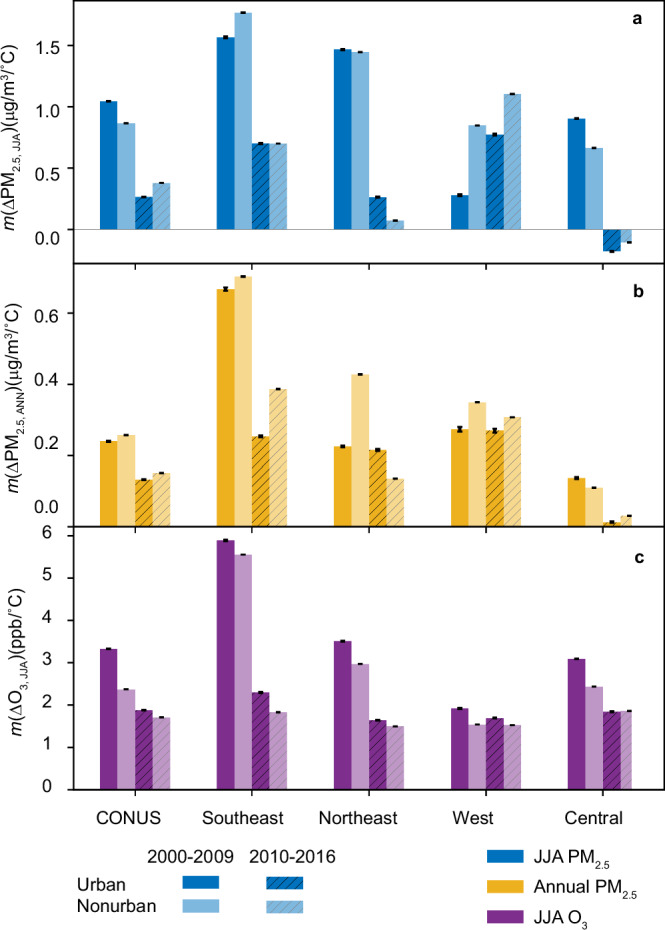
Error bars represent 95% confidence intervals. Temperature sensitivity of summertime PM_2.5 (a), annual PM_2.5 (b), and summertime O₃ (c). All regression coefficients are statistically significant (p < 0.05). The p values are included in Supplementary data.

For PM_2.5, the differences in temperature sensitivity and changes between urban and non-urban areas are complicated. During 2000–2009, m(∆PM_{2.5, JJA}) was higher in non-urban areas in the Southeastern and Western US while higher in urban areas in the Northeastern and Central US (Fig. 4a). This result is within expectation if considering the primary driver of PM_2.5 sensitivity in these regions. PM_2.5 sensitivity in the Southeastern and Western US is driven by pollutants of natural origin (e.g., biogenic SOA and wildfire emissions). In contrast, in the Northeastern and Central US, it is driven by pollutants of anthropogenic origin (e.g., sulfate). After 2010, there was a substantial decrease in both urban and nonurban m(∆PM_{2.5, JJA}) across most regions due to the large decrease in the temperature sensitivity of inorganic components (Supplementary Fig. 6). In the Central US, negative m(∆PM_{2.5, JJA}) was estimated for both urban and non-urban areas. In the Southeastern US, m(∆PM_{2.5, JJA}) are comparable between urban and non-urban areas. However, in the Northeastern US, the urban summer PM_2.5 sensitivity exceeded the nonurban sensitivity, potentially attributable to contributions from temperature-dependent anthropogenic VOC emissions, which were demonstrated to have not been effectively controlled^40,41,67. Recent studies have also suggested that the isoprene and monoterpene emissions exhibit greater temperature dependence in more densely populated areas, further contributing to the higher m(∆PM_{2.5, JJA}) observed in urban grids in the Northeastern US⁶⁸. Studies have shown that the temperature sensitivities calculated from seasonal mean data have the largest spatial variability compared with those calculated from hourly and daily data⁶⁹. An explanation could be that the day-to-day variability significantly depends on synoptic weather systems, whereas long-term response may also reflect the influence of local emissions. For example, although the m(∆PM_{2.5, JJA}) obtained from all urban grids across each region decreased from 2000–2009 to 2010–2016, it may not hold true for a specific urban core. An unexpected increase in m(∆PM_{2.5, JJA}) was observed in metropolitan areas such as Atlanta and Seattle from 2000–2009 to 2010–2016 (Supplementary Fig. 8), which necessitates future studies. It is important to note that the derived temperature sensitivities for individual 1 × 1 km grids within these two areas were not statistically significant, nor were those derived from site observations. More data are required to obtain a robust conclusion at the individual grid level. Regarding the temperature sensitivity of annual PM_2.5, significant reductions were observed in the Southeastern and Central US. The decline in regional aggregated m(∆PM_{2.5, ANN}) in the Northeast was predominantly driven by decreasing sensitivity in nonurban areas, whereas the urban m(∆PM_{2.5, ANN}) remains stable. This is consistent with the increased m(∆PM_{2.5, ANN}) observed in many metropolitan areas, such as New York, Philadelphia, Baltimore, Washington, Hartford, Boston, Buffalo, etc. (Supplementary Fig. 9). The stable m(∆PM_{2.5, ANN}) may reflect the influences of extended summer, increased late-winter and spring temperature variability and faster warming rate along the coastal areas^70–72. These factors may act to counterbalance the effects of emission reductions. High urban m(∆PM_{2.5, ANN}) could also suggest the predominant contribution of OA sensitivity to the annual PM_2.5-temperature relationship, emphasizing the crucial role of aforementioned temperature-dependent VOCs emissions from anthropogenic activities in the temperature sensitivity of OA.

As opposed to the decreasing sensitivity in the Eastern US, the temperature sensitivity of PM_2.5 in the Western US showed an increasing trend. For example, m(PM_{2.5, JJA}) increased from 0.9 (before 2010) to 1.2 µg/m³/°C (after 2010) in the West. Although sparse site measurements do not show statistically significant differences, ML data with complete coverage revealed significant increases in regional m(∆PM_{2.5, JJA}) (Fig. 3d1). In the Northwestern US, where wildfire emissions are the primary source of air pollution, warmer summers are associated with higher PM_2.5 levels. This increase is driven by the heightened sensitivity of OA to temperature (Supplementary Fig. 6). Specifically, a 1 °C rise in summer temperature between 2010–2016 resulted in a greater increase in POA concentrations from wildfires compared to 2000–2009. This increased temperature sensitivity suggests that the local ecosystem is becoming more vulnerable to climate change, which may lead to higher wildfire risks in the future. In addition to local air quality impacts, pollutants from wildfire smoke can be transported over long distances, episodically affecting air quality in other regions^73,74.

Interestingly, while summer PM_2.5 levels in the Western US are higher in non-urban areas compared to urban areas in both periods, a more dramatic increase in temperature sensitivity was observed in urban areas (Fig. 4a). This suggests that wildfire emissions are playing an increasingly important role in urban air quality as anthropogenic emissions decline⁷⁵. Another factor may be that as burned areas expand or more people move to fire-prone regions, more individuals are living closer to wildfires⁷⁶. While summer PM_2.5 sensitivity has increased, the annual PM_2.5 sensitivity in the Western US has remained relatively stable. In contrast to summer OA, the sensitivity of annual OA to summer temperature remains stable during 2000–2022 (Supplementary Fig. 6). This is because the contribution of wildfire emissions to total annual PM_2.5 is less pronounced than in the summer, with biogenic and anthropogenic sources of secondary organic aerosols (SOA) playing a larger role during other seasons. The stable temperature sensitivity of annual OA levels, coupled with the lower relative impact of temperature-sensitive wildfire emissions in non-summer months, helps maintain a stable m(∆PM_2.5,ANN) overall.

Because the ML-modeled data are only available for 2000–2016, the analysis based on high-resolution data was limited to this 17-year period. Although this period also corresponds to the most rapid decrease in anthropogenic emissions and the most significant improvement in air quality in the US (Supplementary Figs. 3 and 5), extending the analysis to more recent years would be helpful to validate our conclusions further. Therefore, ground-based observations from 2017–2022 were used to calculate sensitivities after 2016. The comparison of results for the period 2000–2009, 2010–2019, and 2010–2022 reveals a substantial decrease in summer/annual PM_2.5 and components sensitivities in the Eastern US, contrasting with an increase in the Western US after 2009. This demonstrates that our findings are robust and not affected by the unequal length of the two periods (Supplementary Figs. 6 and 10). Temperature sensitivity of O₃ continues to decline in the Northeastern and Central US, but it remains relatively stable in the Southeastern US after a sharp decline in 2010. The contrasting trends observed across different regions of the US are further illustrated in Fig. 5 and Supplementary Fig. 11, which shows the temperature sensitivity of PM_2.5, O₃, and PM_2.5 species over 19 5-year periods spanning from 2000 to 2022. The decreasing trend in PM_2.5 sensitivity persisted in the Eastern US after 2016. However, the temperature sensitivity of PM_2.5 in the Western US has been rapidly increasing since 2016, suggesting that wildfire emissions are increasingly sensitive to climate warming. The sensitivity of summer/annual PM_2.5 to temperature in the Central US has been on the rise since 2015, driven by increasing OA sensitivity (Supplementary Fig. 11). It is suggestive of the expanding influence of wildfires. Decreasing O₃ sensitivity also extends to recent periods in most regions, except for the Southeastern US. The substantial interannual variability in the O₃-temperature relationship in the Southeastern US could be related to large-scale meteorology^20,77, resulting in a stable and relatively high positive sensitivity after 2010 in this region.

Fig. 5. Temperature sensitivity for each 5-year running time window derived from ML-modeled data (2000–2016, 13 time periods) and ground-based observations (2000–2022, 19 time periods).

The shaded area represents a 95% confidence interval. Temperature sensitivity of summertime PM_2.5 (a1–e1), annual PM_2.5 (a2–e2), and summertime O₃ (a3–e3) in CONUS (a), Southeastern US (b), Northeastern US (c), Western US (d), and Central US (e). The p values are included in Supplementary data.

Implications for the US population exposure

Traditional methods of assessing pollutant concentration exposure typically emphasize the exposure of absolute concentrations of pollutants. Instead, we evaluate human exposure by focusing on temperature sensitivity, which reflects how fluctuations in temperature influence pollutant concentrations and how these temperature-driven changes affect population exposure. The significance of this approach lies in its ability to capture the dynamic nature of air pollution in relation to temperature variability, particularly in the context of climate change. As global temperatures rise, understanding how sensitive pollutant concentrations are to temperature becomes crucial for predicting future exposure risks and developing effective mitigation strategies. By focusing on temperature sensitivity, we can identify populations that may be disproportionately affected by temperature-induced changes in pollutant levels, allowing for more targeted public health interventions. This method also provides insights into the underlying mechanisms that drive variations in pollutant exposure, which can differ significantly from the mechanisms influencing absolute pollutant concentrations.

The high-resolution temperature sensitivity maps allow us to assess the human exposure and vulnerability of the US population to a warming climate. Combined with high-resolution gridded population data (see Methods), we found that the area where air pollution is highly sensitive to summer temperature decreased substantially over the studied period, thereby reducing population exposure to deteriorated air quality induced by climate warming (Fig. 6). Decreases can be found at all exposure levels, with the most significant changes occurring in 75% and 95% of the population exposure levels in most regions (Fig. 6a3–c3), suggesting substantial decreases in relatively high temperature sensitivities. To assess the changes in exposure to high sensitivities, we used the temperature sensitivities (calculated based on data from 2000–2016) to which 75% of the population is exposed as a threshold representing high temperature sensitivity (see “Methods”).

Fig. 6. Number and regional distribution of population exposed to air pollution changes associated with 1 °C change in summer temperature for 2000–2009 and 2010–2016.

Stacked area plots showing the fraction of population living in areas with different levels of temperature sensitivity of summertime PM_2.5 (a), annual PM_2.5 (b), and summertime O₃ (c) during 2000–2009 (a1, b1, c1), 2010–2016 (a2, b2, c2), and box plots showing the temperature sensitivity to which 5%, 25%, 50%, 75%, and 95% of the population is exposed, with light colors represent values in 2010–2016 (a3, b3, c3).

Specifically, the fraction of area and population of the CONUS under m(∆PM_{2.5, JJA}) ≥ 1 µg/m³/°C decreased by 30.1% and 51.2% from 2000–2009 to 2010–2016, respectively (Fig. 6a1, a2, Supplementary Fig. 12a1, a2 and Tables S1 and S2). Such low shifts were pronounced in all regions except for the Western US. In contrast, the fraction of the population under m(∆PM_{2.5, JJA}) ≥ 1 µg/m³/°C increased by 11.1% in the Western US owing to the increased m(∆PM_{2.5, JJA}) in fire-prone areas. The population distribution shifted to a lower O₃-temperature sensitivity due to overall decreases in m(∆O_{3, JJA}) in areas with high population density (Fig. 6c1–c3). The CONUS population under m(∆O_{3, JJA}) ≥ 3 ppb/°C decreased by 82.6% from 2000–2009 to 2010–2016. This improvement was most significant in the Southeast and the Northeast, demonstrating the effectiveness of NO_x emission control in improving public health in climate change. In the Southeastern US, approximately 10% of its population was exposed to m(∆O_{3, JJA}) as high as 7 ppb/°C during 2000–2009. In the period of 2010–2016, 95% of people in this region experienced m(∆O_{3, JJA}) no higher than 4 ppb/°C. The elimination of extremely high O₃-temperature sensitivity in populous areas may drive a substantial reduction in the health burden associated with climate change. Reduction in exposure to m(∆PM_{2.5, ANN}) was less drastic, with a 4.8% decrease in the fraction of the population under m(∆PM_{2.5, ANN}) ≥ 0.5 µg/m³/°C.

Our results demonstrated that anthropogenic emission reductions have successfully reduced the temperature sensitivity of air pollution in densely populated areas, thereby reducing the vulnerability of climate change associated with air pollution. However, the vulnerability to climate change has increased in the fire-prone regions in the Western US. From 2000–2009 to 2010–2016, the temperature sensitivity of PM_2.5 increased in fire-prone areas but decreased in the most densely populated west coast due to anthropogenic emission reductions (Fig. 3a3–b3). The large decrease in more populated areas can also be seen in the significant reduction in exposure level for 5% of the population versus the small decline in exposure level for 5% of the area (Fig. 6a3–c3 and Supplementary Fig. 12a3–c3). Therefore, emission control is not sufficient to mitigate the adverse effects of climate warming on air pollution in areas most affected by natural sources. It is worth noting that the concentration is also increasing in the northwestern US (Supplementary Fig. 4). The contribution of wildfire to PM_2.5 air quality has been more dominant since 2016 in about three-quarters of states in the CONUS and is likely to grow⁷⁵. The increasing temperature sensitivity should be considered in future wildfire projections.

Despite the substantially reduced temperature sensitivity of sulfate in the Eastern US, the temperature sensitivity of OA changed less. In the Southeastern US, the enhanced BVOC level may be the primary driver for the temperature sensitivity of SOA formation. Although anthropogenic SO₂ and NO_x can influence SOA formation in many aspects and the control of anthropogenic emissions reduced the overall OA level^54,55, the positive correlations between OA and temperature remained in this region. However, the significant decrease in OA sensitivity and a larger reduction in non-urban areas in the Northeastern and Central US indicated that there might be a threshold of BVOC and sulfate/NO_x ratio below which the SOA formation would be more sensitive to anthropogenic emission reductions. Furthermore, exposure to m(PM_{2.5, ANN}) increased in the Northeastern US, home to over 30% of the US population. Although the total area with high annual PM_2.5 sensitivity decreased, the fraction of the population exposed to m(∆PM_{2.5, ANN}) ≥ 0.5 µg/m³/°C increased by 18.7% due to increased m(∆PM_{2.5, ANN}) in densely populated east coast areas (Fig. 6b1–b3 and Supplementary Tables 1 and 2). As a caveat, the sensitivity of annual OA level, which might be responsible for the increased m(∆PM_{2.5, ANN}) in the Northeast, showed large uncertainties (Supplementary Fig. 6a2–e2).

Discussion

Understanding the sensitivity of surface air pollution to temperature changes is crucial for predicting future air quality trends in response to climate change and assessing the associated health burden. By leveraging long-term, high-resolution PM_2.5 and O₃ estimates derived from machine learning models, we analyze air quality responses to summer temperature throughout the contiguous US. The machine learning datasets not only successfully reproduced the temperature sensitivities of PM_2.5 and O₃ observed at ground stations but also provided more comprehensive spatial coverage and, thus, better representations of regional sensitivities and human exposure estimates. The high-resolution data generated for the historical temperature sensitivities of PM_2.5 and O₃ are helpful in evaluating the performance of chemical transport models. Demographic information, such as race and ethnicity, income, education, etc., can be used with the high-resolution dataset to characterize the population exposure more thoroughly.

Our results highlight that the positive correlations between PM_2.5 and O₃ and temperature were historically widespread in the contiguous US. However, the deterioration of air quality due to a warmer summer has been effectively abated by anthropogenic emission reductions in the Eastern US, suggesting that a reduction in anthropogenic emissions can efficiently mitigate the adverse health impacts of climate change. The temperature sensitivity of sulfate (and associated ammonium), which is most responsive to emission reduction, has almost vanished during the past decade. Consequently, the temperature sensitivity of inorganics displays a negligible contribution to the overall PM_2.5 sensitivity during 2010–2021. This result implies that further decreases in the temperature sensitivity of inorganics are likely to be more challenging as there is little room for emission reductions, and the summertime SO₂ emissions and sulfate concentrations have remained relatively stable after 2016 (Supplementary Fig. 3). The significant decrease in sulfate sensitivity leaves the OA a dominant contributor to the temperature sensitivity of PM_2.5. Therefore, deteriorated PM_2.5 due to temperature rise remained prominent in the Southeastern and Western US in 2010–2016. The remaining strong temperature response of OA in the Southeast indicates that biogenic SOA formation is insensitive to the change of anthropogenic emissions, although anthropogenic SO₂ and NO_x can enhance SOA formation⁵⁵. The strong positive correlation between O₃ and temperature in the Southeast is highly sensitive to anthropogenic emissions and has been substantially mitigated by reductions in NO_x emissions over the studied period. Although the decreasing trend in NO_x emission has slowed (Supplementary Fig. 3), substantial decreases have been achieved in most regions. In three of four of our studied areas, the O₃-temperature sensitivity has decreased to negative in recent years (Fig. 5). O₃ concentration may plateau or decrease under extremely high temperatures (>312 K), likely due to the enhanced non-stomatal dry deposition, diminished role of NO_x sequestration by PAN, reduced NO-titration effect, and reduced biogenic emissions^28,65,78. It is unclear if this phenomenon could be responsible for the negative response of seasonal mean O₃ concentration to temperature. However, complex chemical and biophysical feedback needs to be considered in predicting the response of O₃ to climate change. The remaining temperature sensitivity of O₃ may reflect meteorological factors that are covariant with temperature, and further studies are required to disentangle the relative contributions. Our primary results hold for most months, but it is worth noting that increased sensitivity is seen in transition periods (e.g., May and October, Supplementary Figs. 13 and 14). For example, the temperature sensitivity of spring O₃ over the eastern US has been on the rise in recent years (Fig. 14b4–c4). Despite an overall decline in summer ozone levels, it is important to highlight an increase in O₃ concentration and associated human exposure during shoulder seasons⁷⁹. The simultaneously increasing temperature response intensifies the health concerns associated with O₃ exposure. This emphasizes the necessity for further investigations into O₃ levels and temperature responses during transition months, which are experiencing warming trends attributable to climate change⁷⁰.

The increasing trend of PM_2.5-temperature sensitivity in the Western US suggests that wildfire emissions have become more sensitive to temperature anomalies in recent years under rapid climate change. Potential factors contributing to the exacerbated temperature response of wildfire emissions include more fire occurrences, larger burning areas, longer fire durations, etc. The mechanisms underpinning this phenomenon are worth further investigation. Additionally, the temperature sensitivity of the fall (September, October, and November) PM_2.5 has spiked since 2016 (Supplementary Fig. 14d2). This result is consistent with studies suggesting that the wildfire season is extending in a warmer climate^80,81. Given the escalating temperature sensitivity of PM_2.5 in this region (Fig. 5), a higher risk of human exposure and health impact is expected in recent years and beyond. Our results for the Western US highlight an urgent need for effective fire management in this region. We acknowledge that the r² values for ground measurements and ML estimations of PM_2.5 at certain monitoring sites in the Western US are relatively low. This could be attributed to mountainous terrain, which can adversely affect the model performance. For annual concentrations, r² values range from 0.4 to 0.7⁴². However, it is worth noting that the r² values for summer and fall PM_2.5 at most sites across the northwest exceed 0.8. This indicates that the ML models effectively capture the impact of wildfires during fire seasons. Furthermore, our results also demonstrated that the temperature sensitivities derived from ML data are consistent with those obtained from available ground-based observations on both magnitudes and trends.

Few studies focus on the PM_2.5-temperature relationship and its changes with emission reduction due to the different responses of PM components^22,29,30,39. The detailed analysis of the PM_2.5-temperature relationship in this study can be useful for model development and validation. We compared the temperature sensitivity of PM_2.5 in urban and non-urban areas and discussed the possible mechanism driving the differences in magnitude and trend for the first time. The higher temperature sensitivity of O₃ in urban areas has decreased over the past decade, reducing the difference between urban and non-urban areas and potentially contributing to air pollution exposure equality. Conversely, a larger increase in PM_2.5 sensitivity was found in urban areas in the Western US. Although the temperature sensitivity of annual PM_2.5 is relatively low, it remains stable in the urban areas of the northeastern US. However, these trends are not observed in ground-based PM_2.5 and its species measurements, underscoring the usefulness of high-resolution datasets. For future air quality projections, correctly capturing the temperature-sensitive processes can be more important than reproducing the observed concentrations³⁰. Considering the radiative effects of aerosols, these processes can also be critical for modeling climate-aerosol feedback⁸². Although we expect minimized impacts from sulfate aerosol with continually decreasing sulfur dioxide emissions, the sensitivity associated with OA remains significant. Most organic species scatter solar radiation, while there are also light-absorbing components of organic aerosol known as “brown carbon”⁸³. Therefore, future climate projections must consider the temperature responses of OA and its radiative effects^84,85. In addition, the formation pathways of SOA exhibit distinct optimal temperatures, leading to diverse SOA composition and, thus, aerosol properties under different environmental conditions^86,87. One limitation of this study is that we used ground-based measurements of PM_2.5 species concentrations to diagnose the temperature sensitivity of these species to investigate the main drivers of overall PM_2.5 sensitivity. Spatially sparse measurements of species concentrations limit their regional representativeness (as represented by large error bars in Supplementary Fig. 6). Moreover, this approach cannot adequately account for the disparate trends observed in metropolitan areas. In addition, due to data availability, species and PM_2.5 concentrations were not necessarily collected from the same sites or on the same days, leading to differences in changes in PM_2.5 and changes in summed species concentrations. Future work can benefit from the emerging high-resolution PM_2.5 species dataset from machine learning models⁸⁸, and more accurate analyses can be performed to improve understanding of the response of PM_2.5 to temperature rising.

Negative temperature sensitivities observed in certain locations may be linked to meteorological factors that covary with temperature. Elevated temperatures promote the partitioning of semi-volatile compounds into the gas phase, contributing to a decrease in nitrate and organic aerosol concentrations. Recent studies highlight that terpene emissions contribute ~60% of VOC OH reactivity, O₃, and SOA formation potential¹⁵. Chamber studies show that lower temperatures enhance SOA production through the ozonolysis of monoterpenes⁵⁶. This negative temperature dependence may be compensated by increased emission at higher temperatures. Negative O₃-temperature sensitivities are rare and may be due to the nonlinear response of ozone formation to precursor changes. We acknowledge that our current results do not fully capture the drivers behind these negative values. Additional years of data are necessary to obtain more robust conclusions, and chemical transport models are essential for quantitatively assessing the influence of various processes.

Many processes contribute to the temperature sensitivity of air quality, for instance, precursor emissions, chemical reaction rate, stagnation, deposition, etc.¹⁶. Another limitation of our study is that the utilization of observed and machine learning modeled PM_2.5 and O₃ concentration data can only provide information on the total derivative of air pollution and temperature (d[O₃]/dT, d[PM_2.5]/dT, d[OA]/dT). While we proposed potential mechanisms to interpret our findings, chemical transport models are required to break down the total sensitivity and quantify contributions from the individual processes, i.e., stagnation (∂[PM_2.5]/∂[stagnation]* ∂[stagnation]/∂[T]), biogenic VOC emissions (∂[OA]/∂[BVOC]* ∂[BVOC]/∂[T]), anthropogenic SO₂ emissions (∂[sulfate]/∂[SO₂]* ∂[SO₂]/∂[T]), etc.⁸⁹. However, one prerequisite to understanding the process contribution is that models can reproduce the observed total derivative. In this sense, the high-resolution data generated in this study can be applied to evaluate the temperature sensitivity simulated by CTMs. By comparing our observations with CTM outputs, we can identify the primary biases in CTM simulations, such as over- or underestimation of temperature sensitivity in specific regions or pollutant types. These biases can arise from various factors, including inaccuracies in representing emissions, chemical processes, or meteorological influences within the models. Once identified, these mechanisms can be optimized in the models, leading to improved performance and more accurate predictions of air quality under changing climate conditions. It is important to note that the machine learning models are trained on historical temperature ranges, which may limit their applicability to the extreme temperatures anticipated in future climate scenarios. As a result, the temperature-sensitivity processes simulated by CTMs under extreme conditions cannot be fully evaluated by the ML-modeled results. This limitation can be mitigated by evaluating historical temperature-air pollution relationships across various temperature ranges to capture the non-linear response of air pollution to temperature under extreme conditions. In addition, the air pollution-temperature relationships and primary drivers can differ depending on the timescale (e.g., daily measurements or monthly/seasonal averages). Daily data highlights the effects of stagnation related to synoptic weather systems, such as the cold front in the northern US and Bermuda High in the southeastern US^23,50. In contrast, the effects of chemistry on the magnitude tend to be significant when considering long-term average air pollution levels, which are more crucial to air pollution-climate interactions and human health than day-to-day variations^20,28,32. Our results also indicate that the statistical relationships for future projections built upon historic observations need to consider complex interactions of air quality and climate with changing anthropogenic emissions. In addition to temperature, many other meteorological parameters, such as precipitation and wind speed, can also play an important role in such interactions.

Methods

High-resolution PM_2.5/O₃ concentration and temperature data

Ground-level daily mean PM_2.5 and 8-h maximum O₃⁴³ across the contiguous United States were generated using an ensemble machine-learning approach in previous studies^42,43. Briefly, three machine learning algorithms (neural network, random forest, and gradient boosting) were trained based on multiple predictor variables, including satellite data, meteorological variables, land-use variables, elevation, chemical transport model simulations, reanalysis datasets, and others. The PM_2.5 and O₃ concentrations were modeled with each algorithm. A geographic-weighted generalized additive model combined estimates and obtained an overall prediction. The ensemble model demonstrates good performance with a 10-fold cross-validated R² of 0.86 for daily PM_2.5 predictions, 0.89 for annual PM_2.5 predictions, and 0.90 for daily maximum 8 h O₃. The average RMSE (root mean square error) was 2.79 μg/m³ for daily PM_2.5 and 4.55 ppb for daily maximum 8 h O₃, respectively. The spline fit between daily PM_2.5 predictions and measurements was close to 1:1, including the rarely occurring concentration of 60 μg/m³, indicating good performance over the range of concentrations with fewer monitoring data. We further conducted validations for the original data (Supplementary Fig. 15a–c) and separately for spatial (long-term mean, Supplementary Fig. 15d–f) and temporal (anomalies, Supplementary Fig. 15g–i) variations. The r value ranges from 0.95 to 0.99, indicating good performance. Detailed information on PM_2.5 and O₃ datasets can be found in Di et al.⁴² and Requia et al.⁴³, respectively.

Both datasets have a spatial resolution of 1 km × 1 km. The temporal resolution is daily. Gridded daily maximum and minimum temperatures are obtained from Daymet Daily Surface Weather Data on a 1 km × 1 km Grid for North America, Version 4 R1 (10.3334/ORNLDAAC/2129). The mean temperature is calculated by summing the maximum and minimum temperatures and dividing by 2.

Ground-based observations

Daily measurements of O₃, PM_2.5, and particulate components (sulfate, nitrate, ammonium, organic carbon, and elemental carbon) were obtained from the Air Quality System (AQS) network managed by US Environmental Protection Agency (EPA)⁴⁴, The Interagency Monitoring of Protected Visual Environments (IMPROVE)⁹⁰ and The SouthEastern Aerosol Research and Characterization (SEARCH)⁹¹. A factor of 2.1 was used to convert organic carbon mass concentration to organic aerosol mass concentration^92,93. The O₃, PM_2.5, and PM components measurements were obtained from 1796, 1469, and 713 sites, respectively. The pollutant samples are collected for 24 h every 3 days at most sites. Only data that met the following criteria were included in the sensitivity analysis. Monthly mean concentrations are calculated for months with more than 6 daily measurements. Summer mean concentrations are computed for the summer with at least two monthly data for July, August, or September. Annual mean concentrations are calculated for the year with more than eight monthly mean data. The sensitivity diagnosis was only performed for monitoring stations with at least 11 years of summer or annual mean measurements during 2000–2016. Consequently, O₃ data from 997 sites, PM_2.5 data from 567 sites, and species data from 381 sites were used in sensitivity analyses. The number of measurements used in linear regression was listed in Supplementary Tables 3 and 4.

Temperature observations are from Global Summary of the Month (GSOM), Version 1, provided by the National Centers for Environmental Information (NCEI, https://www.ncei.noaa.gov/access). NCEI stations within 30 km of AQS stations are averaged and considered co-located pollutant and temperature measurements. The criteria used to select AQS data for the summer averages calculation and sensitivity examination were also applied to the NCEI temperature data processing.

Gridded population dataset

The gridded population distribution of the US is from the UN WPP-adjusted population count/density, v4.11 product provided by Gridded Population of the World (GPW), v4 database (https://sedac.ciesin.columbia.edu/data/collection/gpw-v4). Data at the native 30 arc-second (approximately 1 km) resolution are used. The population dataset was matched with the high-resolution air pollution datasets by the nearest central grids. The 2010 and 2020 population count data at 30 arc-second resolution was used to assess changes in population exposure from 2000–2009 to 2010–2016.

Quantification of air pollution sensitivity to summer temperature

Following the methodology described by Fu et al.²⁰, the sensitivity of air pollution to temperature is calculated as the slope of the linear regression line for detrended air pollutant concentration anomalies (e.g., ∆PM_2.5) and detrended temperature anomalies (∆T). Interannual anomalies of pollutant concentration and temperature were calculated by removing the long-term means. The detrending operation to eliminate the apparent associations between air pollution and temperature due to long-term trends. For example, a decreasing long-term trend of PM_2.5 and an increasing trend in temperature will cause a negative association in the analysis without detrending, which will mask the causal relationships between PM_2.5 and temperature, which are related to chemistry, emission, and transport. We focused on the temperature sensitivity of O₃ and PM_2.5 concentrations at ground level due to their direct impacts on public health.

As shown in Supplementary Fig. 13, observations reveal a positive correlation between O₃ and PM_2.5 concentrations and temperature during the warm season (May-October). The temperature sensitivity of PM_2.5 and O₃ in each season, along with its trend, was examined by using ground-based observations, as depicted in Supplementary Fig. 14 (summer results are shown in Fig. 5). Notably, the peak temperature sensitivity is observed during the summer season for both pollutants. In light of the mediation role of air pollution in the increased mortality due to the rise in summer mean temperature^2,94, as well as the co-occurrence of heatwaves and severe air pollution during the summertime that has been observed in many populous regions around the world^23,95, we mainly focused on the responses of summer air pollution (PM_{2.5, JJA} and O_{3, JJA}) to summer temperature changes in this study. While O₃ pollution is mainly a warm-season issue due to photochemical reactions, PM_2.5 is a year-round air quality concern because of the complex seasonal variations¹⁶. To assess the potential lags or long-term effects of warmer summers on air quality, we also investigated the temperature sensitivity of annual average PM_2.5 (PM_{2.5, ANN}) in the 12 months after summers (from June to May of the following year). The temperature sensitivity of summertime PM_2.5, annual PM_2.5, summertime O₃ were denoted as m(∆PM_{2.5, JJA}), m(∆PM_{2.5, ANN}), m(∆O_{3, JJA}), respectively. The sensitivities derived from the high-resolution dataset are based on data from 17 consecutive years (2000–2016), while the observed sensitivities are based on the 11 or more years of data available at each site.

Different regions in the CONUS were investigated separately to illustrate the spatial heterogeneity of pollutant-temperature relationships. The CONUS was divided into four regions (Supplementary Fig. 16): the Southeastern US, the Northeastern US, the Western US, and the Central US. The regional responses were obtained by regressing all detrended air pollution anomalies on temperature anomalies within each region (Supplementary Fig. 17). Data from 10,985,054 grids in the CONUS were used in sensitivity diagnosis, with 1,132,570 grids in the Southeastern US, 1,173,778 grids in the Northeastern US, 4,437,804 grids in the Western US, and 4,240,902 grids in the Central US. For summertime PM_2.5, the R² values from the linear regression with temperature are 0.20 in the Southeastern US, 0.18 in the Northeastern US, 0.23 in the Western US, and 0.06 in the Central US, indicating varying degrees of correlation across regions. For annual PM₂.₅, the R² values are generally lower, at 0.19, 0.10, 0.13, and 0.01 for the Southeastern, Northeastern, Western, and Central US, respectively. In contrast, the R² values for O₃-temperature sensitivity are higher, ranging from 0.31 to 0.45 across regions, suggesting a stronger correlation between temperature and ozone levels than for PM₂.₅. The low to moderate values of R² indicate factors other than temperature, such as fluctuations in emissions, precipitation, and wind speed, can also contribute to the variability of air pollutants. However, the temperature-pollutant relationships remain significant (p < 0.01) as large datasets were used to derive these relationships. The sample sizes of linear regressions were listed in Supplementary Tables 3 and 4. We also adopt a bootstrapping approach to calculate regional sensitivity with 1000 replications. The slope and standard error based on the bootstrapping method were comparable to that based on the linear regression models.

Regional temperature sensitivity derived from ML datasets was comparable to that based on measurements (Fig. 2f–j). Larger discrepancies were found in the Western and Central US due to lower monitoring station coverage. Therefore, data in grids co-locating with observations (within a 5 km radius) were used to validate the ML datasets. After selection, data from 58,237, 55,367, and 98,677 co-located grids were utilized to calculate m(∆PM_{2.5, JJA}), m(∆PM_{2.5, ANN}), and m(∆O_{3, JJA}), respectively. As shown in Supplementary Fig. 18 (compared to Supplementary Fig. 17) and Supplementary Fig. 19 (compared to Fig. 2), the agreement was improved in all regions when only co-located data were used in the analysis. We acknowledge that the ML datasets rely on observations as a training set, so areas with sparse measurements inevitably have larger errors than areas well constrained by observations (e.g., the Western and Central US). However, considering that the ML approach incorporated multi-source datasets (ground observation, satellite observation, and chemical transport models (CTMs)) and successfully reproduced not only the observed long-term concentration but also the magnitude and spatial distribution of temperature sensitivity, we assumed that regional mean sensitivity derived from this dataset would be more representative than the sensitivity derived from sparse ground-based observations.

The varied temperature dependences of its species complicate the PM_2.5-temperature relationship²⁹. The associations between temperature and five principal PM_2.5 components, including sulfate, nitrate, ammonium, organic aerosol (OA), and elemental carbon (EC), were investigated using the long-term observation derived from the AQS database. Sensitivities at each site are shown in Supplementary Fig. 1, and regional sensitivities are displayed in Supplementary Fig. 20. It should be noted that m(∆PM_2.5) obtained from ML data or PM_2.5 measurements is not necessarily equal to the sum of sensitivities of each species because of different locations, numbers, and times of observations used to fit the slopes. The inset pie charts in Fig. 2 (main text) showed species contributions to summed sensitivity. Temperature sensitivity of summer nitrate concentration in the Northeast was negative with a slope of –0.005 µg/m³/°C and thus was not included in the pie chart. As shown in Supplementary Fig. 20, the nitrate sensitivity ranges from –0.005 to 0.024 µg/m³/°C, making a small contribution to the overall PM_2.5 sensitivity.

Anthropogenic emissions were substantially reduced during the past decade. Supplementary Fig. 3 shows the summer emission of SO₂ and NO_x from anthropogenic sources and OC emissions from biomass burning in CONUS and four subregions during 2000–2022. The anthropogenic emission data are from National Emissions Inventory (NEI)⁹⁶ and the biomass burning emission data are from Global Fire Emission Database, version 4.1 (GFEDv4)⁹⁷. As a result, summer PM_2.5, annual PM_2.5, and summer O₃ concentrations show a decreasing trend in most regions (Supplementary Fig. 5). From 2000–2009 to 2010–2016, the summer PM_2.5, annual PM_2.5, and summer O₃ concentrations in CONUS decreased by 23.6%, 30.5%, and 8.9%, respectively. Likewise, the decreasing trend can be found in the temperature sensitivity of air pollution for the thirteen (nineteen) 5-year periods during 2000–2016 (2000–2022) based on ML data (observations) (Fig. 5).

The impacts of anthropogenic emission reductions on temperature sensitivity were further studied by comparing the sensitivities in 2000–2009 and 2010–2016. The regional sensitivities calculated by the bootstrapping method were used to calculate the percentage change and its confidence interval of each region (Fig. 3d1–d3). The changes in population exposure associated with decreased temperature sensitivity were evaluated by comparing population distribution under different sensitivity levels during 2000–2009 and 2010–2016. The high temperature sensitivities (based on data from 2000–2016) experienced by approximately 25% of the population were selected as the threshold value of high temperature sensitivities. The threshold value for m(∆PM_{2.5, JJA}), m(∆PM_{2.5, ANN}), m(∆O_{3, JJA}) are 1 µg/m³/°C, 0.5 µg/m³/°C, and 3 ppb/°C, respectively. Because of the unevenly distributed population, the area distribution was also studied to show the exposure changes in the US.

The difference in the temperature sensitivity of O₃ concentration in urban and non-urban areas was examined. The urban/nonurban grids were identified using the GPW population density data in 2010 and 2020. Grids with a population density ≥400 people/km² are considered urban grids⁹⁸.

Author contributions

P.L. conceived the study. L.Y. performed the data collection and data analysis. L.Y. wrote the first draft of the manuscript. P.L., B.B., B.Z., Q.Z., Q.D., W.R., J.S., and L.S. contributed to subsequent versions and the further interpretation of the data and results. All authors reviewed and approved the final version of the manuscript.

Data availability

High-resolution daily mean PM_2.5 and 8-h maximum ozone datasets are publicly available at NASA Socioeconomic Data and Applications Center^42,43,99,100. Gridded temperature data are from Daymet Daily Surface Weather Data on a 1-km Grid for North America, Version 4 R1 (10.3334/ORNLDAAC/2129)¹⁰¹. Daily O₃, PM_2.5, and particulate component measurements were obtained from the Air Quality System (AQS) network (https://aqs.epa.gov/aqsweb/airdata/download_files.html). Temperature observations are from Global Summary of the Month (GSOM), Version 1, provided by the National Centers for Environmental Information (NCEI, https://www.ncei.noaa.gov/access). Gridded population distribution of the US is from the UN WPP-adjusted population count/density, v4.11 product provided by Gridded Population of the World (GPW), v4 database (https://sedac.ciesin.columbia.edu/data/collection/gpw-v4)¹⁰². Other data that support the plots and other findings of this work are available at 10.5281/zenodo.8109660.

Code availability

All code used to produce the analysis is available at the following repository: 10.5281/zenodo.8109660. The details of implementation can be found in “Methods”.

Competing interests

The authors declare no competing interests.

Supplementary information

The online version contains supplementary material available at 10.1038/s41612-024-00862-4.

References

- 1.Romanello, M. et al. The 2021 report of the Lancet Countdown on health and climate change: code red for a healthy future. Lancet398, 1619–1662 (2021). [DOI] [PMC free article] [PubMed] [Google Scholar]
- 2.Shi, L., Kloog, I., Zanobetti, A., Liu, P. & Schwartz, J. D. Impacts of temperature and its variability on mortality in New England. Nat. Clim. Change5, 988–991 (2015). [DOI] [PMC free article] [PubMed] [Google Scholar]
- 3.Shi, L. et al. Chronic effects of temperature on mortality in the Southeastern USA using satellite-based exposure metrics. Sci. Rep.6, 30161 (2016). [DOI] [PMC free article] [PubMed] [Google Scholar]
- 4.Costello, A. et al. Managing the health effects of climate change: Lancet and University College London Institute for Global Health Commission. Lancet373, 1693–1733 (2009). [DOI] [PubMed] [Google Scholar]
- 5.Mora, C. et al. Global risk of deadly heat. Nat. Clim. Change7, 501–506 (2017). [Google Scholar]
- 6.Vicedo-Cabrera, A. M. et al. The burden of heat-related mortality attributable to recent human-induced climate change. Nat. Clim. Change11, 492–500 (2021). [DOI] [PMC free article] [PubMed] [Google Scholar]
- 7.Ebi, K. L. et al. Hot weather and heat extremes: health risks. Lancet398, 698–708 (2021). [DOI] [PubMed] [Google Scholar]
- 8.Wu, S. et al. Effects of 2000-2050 global change on ozone air quality in the United States. J. Geophys. Res. Atmos113, 302 (2008). [Google Scholar]
- 9.Murray, C. J. L. et al. Global burden of 87 risk factors in 204 countries and territories, 1990–2019: a systematic analysis for the Global Burden of Disease Study 2019. Lancet396, 1223–1249 (2020). [DOI] [PMC free article] [PubMed] [Google Scholar]
- 10.Akimoto, H. & Tanimoto, H. Rethinking of the adverse effects of NOx-control on the reduction of methane and tropospheric ozone—challenges toward a denitrified society. Atmos. Environ.277, 119033 (2022). [Google Scholar]
- 11.Jhun, I., Coull, B. A., Zanobetti, A. & Koutrakis, P. The impact of nitrogen oxides concentration decreases on ozone trends in the USA. Air Qual. Atmos. Health8, 283–292 (2015). [DOI] [PMC free article] [PubMed] [Google Scholar]
- 12.Simon, H., Reff, A., Wells, B., Xing, J. & Frank, N. Ozone trends across the United States over a period of decreasing NOx and VOC emissions. Environ. Sci. Technol.49, 186–195 (2015). [DOI] [PubMed] [Google Scholar]
- 13.Lee, C. & Yoon, J. Temperature dependence of hydroxyl radical formation in the hv/Fe3+/H2O2 and Fe3+/H2O2 systems. Chemosphere56, 923–934 (2004). [DOI] [PubMed] [Google Scholar]
- 14.Li, J. et al. Effects of OH radical and SO2 concentrations on photochemical reactions of mixed anthropogenic organic gases. Atmos. Chem. Phys.22, 10489–10504 (2022). [Google Scholar]
- 15.Pfannerstill, E. Y. et al. Temperature-dependent emissions dominate aerosol and ozone formation in Los Angeles. Science384, 1324–1329 (2024). [DOI] [PubMed] [Google Scholar]
- 16.Jacob, D. J. & Winner, D. A. Effect of climate change on air quality. Atmos. Environ.43, 51–63 (2009). [Google Scholar]
- 17.Zhang, Y. et al. Diurnal climatology of planetary boundary layer height over the contiguous United States derived from AMDAR and reanalysis data. J. Geophys. Res. Atmos.125, e2020JD032803 (2020). [Google Scholar]
- 18.Budakoti, S. & Singh, C. Examining the characteristics of planetary boundary layer height and its relationship with atmospheric parameters over Indian sub-continent. Atmos. Res.264, 105854 (2021). [Google Scholar]
- 19.Bloomer, B. J., Stehr, J. W., Piety, C. A., Salawitch, R. J. & Dickerson, R. R. Observed relationships of ozone air pollution with temperature and emissions. Geophys. Res. Lett.36, 803 (2009). [Google Scholar]
- 20.Fu, T.-M., Zheng, Y., Paulot, F., Mao, J. & Yantosca, R. M. Positive but variable sensitivity of August surface ozone to large-scale warming in the southeast United States. Nat. Clim. Change5, 454–458 (2015). [Google Scholar]
- 21.Fiore, A. M., Naik, V. & Leibensperger, E. M. Air quality and climate connections. J. Air Waste Manag. Assoc.65, 645–685 (2015). [DOI] [PubMed] [Google Scholar]
- 22.Westervelt, D. M. et al. Quantifying PM2.5-meteorology sensitivities in a global climate model. Atmos. Environ.142, 43–56 (2016). [Google Scholar]
- 23.Schnell, J. L. & Prather, M. J. Co-occurrence of extremes in surface ozone, particulate matter, and temperature over eastern North America. Proc. Natl Acad. Sci. USA114, 2854–2859 (2017). [DOI] [PMC free article] [PubMed] [Google Scholar]
- 24.Fu, T.-M. & Tian, H. Climate change penalty to ozone air quality: review of current understandings and knowledge gaps. Curr. Pollut. Rep.5, 159–171 (2019). [Google Scholar]
- 25.Cohen, A. J. et al. Estimates and 25-year trends of the global burden of disease attributable to ambient air pollution: an analysis of data from the Global Burden of Diseases Study 2015. Lancet389, 1907–1918 (2017). [DOI] [PMC free article] [PubMed] [Google Scholar]
- 26.Nolte, C. G. et al. Regional temperature-ozone relationships across the U.S. under multiple climate and emissions scenarios. J. Air Waste Manag. Assoc.71, 1251–1264 (2021). [DOI] [PMC free article] [PubMed] [Google Scholar]
- 27.Porter, W. C., Heald, C. L., Cooley, D. & Russell, B. Investigating the observed sensitivities of air-quality extremes to meteorological drivers via quantile regression. Atmos. Chem. Phys.15, 10349–10366 (2015). [Google Scholar]
- 28.Romer, P. S. et al. Effects of temperature-dependent NOx emissions on continental ozone production. Atmos. Chem. Phys.18, 2601–2614 (2018). [Google Scholar]
- 29.Tai, A. P. K., Mickley, L. J. & Jacob, D. J. Correlations between fine particulate matter (PM2.5) and meteorological variables in the United States: implications for the sensitivity of PM2.5 to climate change. Atmos. Environ.44, 3976–3984 (2010). [Google Scholar]
- 30.Shen, L., Mickley, L. J. & Murray, L. T. Influence of 2000–2050 climate change on particulate matter in the United States: results from a new statistical model. Atmos. Chem. Phys.17, 4355–4367 (2017). [Google Scholar]
- 31.Ito, A., Sillman, S. & Penner, J. E. Global chemical transport model study of ozone response to changes in chemical kinetics and biogenic volatile organic compounds emissions due to increasing temperatures: sensitivities to isoprene nitrate chemistry and grid resolution. J. Geophys. Res. Atmos114, 301 (2009). [Google Scholar]
- 32.Porter, W. C. & Heald, C. L. The mechanisms and meteorological drivers of the summertime ozone–temperature relationship. Atmos. Chem. Phys.19, 13367–13381 (2019). [Google Scholar]
- 33.Vannucci, P. F. et al. Temperature-dependent composition of summertime PM2.5 in observations and model predictions across the Eastern U.S. ACS Earth Space Chem.8, 381–392 (2024). [DOI] [PMC free article] [PubMed] [Google Scholar]
- 34.Coates, J., Mar, K. A., Ojha, N. & Butler, T. M. The influence of temperature on ozone production under varying NOx conditions—a modelling study. Atmos. Chem. Phys.16, 11601–11615 (2016). [Google Scholar]
- 35.Meng, X. et al. Chemical drivers of ozone change in extreme temperatures in eastern China. Sci. Total Environ.874, 162424 (2023). [DOI] [PubMed] [Google Scholar]
- 36.Hand, J. L., Prenni, A. J., Copeland, S., Schichtel, B. A. & Malm, W. C. Thirty years of the Clean Air Act Amendments: impacts on haze in remote regions of the United States (1990–2018). Atmos. Environ.243, 117865 (2020). [Google Scholar]
- 37.Rasmussen, D. J., Hu, J., Mahmud, A. & Kleeman, M. J. The ozone–climate penalty: past, present, and future. Environ. Sci. Technol.47, 14258–14266 (2013). [DOI] [PMC free article] [PubMed] [Google Scholar]
- 38.Pusede, S. E., Steiner, A. L. & Cohen, R. C. Temperature and recent trends in the chemistry of continental surface ozone. Chem. Rev.115, 3898–3918 (2015). [DOI] [PubMed] [Google Scholar]
- 39.Vannucci, P. F. & Cohen, R. C. Decadal trends in the temperature dependence of summertime urban PM2.5 in the Northeast United States. ACS Earth Space Chem.6, 1793–1798 (2022). [Google Scholar]
- 40.Nussbaumer, C. M. & Cohen, R. C. Impact of OA on the temperature dependence of PM 2.5 in the Los Angeles Basin. Environ. Sci. Technol.55, 3549–3558 (2021). [DOI] [PubMed] [Google Scholar]
- 41.Hass-Mitchell, T. et al. Increasing contributions of temperature-dependent oxygenated organic aerosol to summertime particulate matter in New York City. ACS EST Air. 10.1021/acsestair.3c00037 (2024). [DOI] [PMC free article] [PubMed]
- 42.Di, Q. et al. An ensemble-based model of PM2.5 concentration across the contiguous United States with high spatiotemporal resolution. Environ. Int.130, 104909 (2019). [DOI] [PMC free article] [PubMed] [Google Scholar]
- 43.Requia, W. J. et al. An ensemble learning approach for estimating high spatiotemporal resolution of ground-level ozone in the contiguous United States. Environ. Sci. Technol.54, 11037–11047 (2020). [DOI] [PMC free article] [PubMed] [Google Scholar]
- 44.US Environmental Protection Agency. Air Quality System Data Mart [internet database]. https://www.epa.gov/outdoor-air-quality-data. Accessed December 3, 2024.
- 45.Williams, A. P. et al. Observed impacts of anthropogenic climate change on wildfire in California. Earths Future7, 892–910 (2019). [Google Scholar]
- 46.Abel, D. et al. Response of power plant emissions to ambient temperature in the Eastern United States. Environ. Sci. Technol.51, 5838–5846 (2017). [DOI] [PubMed] [Google Scholar]
- 47.Geddes, J. A., Pusede, S. E. & Wong, A. Y. H. Changes in the relative importance of biogenic isoprene and soil NOx emissions on ozone concentrations in nonattainment areas of the United States. J. Geophys. Res. Atmos.127, e2021JD036361 (2022). [Google Scholar]
- 48.Pusede, S. E. et al. On the temperature dependence of organic reactivity, nitrogen oxides, ozone production, and the impact of emission controls in San Joaquin Valley, California. Atmos. Chem. Phys.14, 3373–3395 (2014). [Google Scholar]
- 49.Lin, M. et al. Vegetation feedbacks during drought exacerbate ozone air pollution extremes in Europe. Nat. Clim. Change10, 444–451 (2020). [Google Scholar]
- 50.Kerr, G. H. et al. Disentangling the drivers of the summertime ozone-temperature relationship over the United States. J. Geophys. Res. Atmos.124, 10503–10524 (2019). [Google Scholar]
- 51.Zhang, X., Waugh, D. W., Kerr, G. H. & Miller, S. M. Surface ozone-temperature relationship: the meridional gradient ratio approximation. Geophys. Res. Lett.49, e2022GL098680 (2022). [Google Scholar]
- 52.Nault, B. A. et al. Secondary organic aerosols from anthropogenic volatile organic compounds contribute substantially to air pollution mortality. Atmos. Chem. Phys.21, 11201–11224 (2021). [Google Scholar]
- 53.Ridley, D. A., Heald, C. L., Ridley, K. J. & Kroll, J. H. Causes and consequences of decreasing atmospheric organic aerosol in the United States. Proc. Natl Acad. Sci. USA115, 290–295 (2018). [DOI] [PMC free article] [PubMed] [Google Scholar]
- 54.Zhang, J. et al. The response of summertime organic aerosol composition to emission controls in the Northeastern United States. J. Geophys. Res. Atmos.127, e2022JD037056 (2022). [Google Scholar]
- 55.Xu, L. et al. Effects of anthropogenic emissions on aerosol formation from isoprene and monoterpenes in the southeastern United States. Proc. Natl Acad. Sci. USA112, 37–42 (2015). [DOI] [PMC free article] [PubMed] [Google Scholar]
- 56.Deng, Y. et al. Temperature and acidity dependence of secondary organic aerosol formation from α-pinene ozonolysis with a compact chamber system. Atmos. Chem. Phys.21, 5983–6003 (2021). [Google Scholar]
- 57.Afrin, S. & Garcia-Menendez, F. The influence of prescribed fire on fine particulate matter pollution in the Southeastern United States. Geophys. Res. Lett.47, e2020GL088988 (2020). [Google Scholar]
- 58.Tao, M. et al. Investigating changes in ozone formation chemistry during summertime pollution events over the Northeastern United States. Environ. Sci. Technol.56, 15312–15327 (2022). [DOI] [PMC free article] [PubMed] [Google Scholar]
- 59.Nussbaumer, C. M. & Cohen, R. C. The role of temperature and NOx in ozone trends in the Los Angeles Basin. Environ. Sci. Technol.54, 15652–15659 (2020). [DOI] [PubMed] [Google Scholar]
- 60.Perdigones, B. C., Lee, S., Cohen, R. C., Park, J.-H. & Min, K.-E. Two decades of changes in summertime ozone production in California’s South Coast Air Basin. Environ. Sci. Technol.56, 10586–10595 (2022). [DOI] [PubMed] [Google Scholar]
- 61.Jin, X., Fiore, A., Boersma, K. F., Smedt, I. D. & Valin, L. Inferring changes in summertime surface ozone–NOx–VOC chemistry over U.S. urban areas from two decades of satellite and ground-based observations. Environ. Sci. Technol.54, 6518–6529 (2020). [DOI] [PMC free article] [PubMed] [Google Scholar]
- 62.Johnson, M. S. et al. Insights into the long-term (2005–2021) spatiotemporal evolution of summer ozone production sensitivity in the Northern Hemisphere derived with the Ozone Monitoring Instrument (OMI). Atmos. Chem. Phys.24, 10363–10384 (2024). [Google Scholar]
- 63.Blanchard, C. L. & Hidy, G. M. Ozone response to emission reductions in the southeastern United States. Atmos. Chem. Phys.18, 8183–8202 (2018). [Google Scholar]
- 64.Li, W. et al. Spatial variation of surface O3 responses to drought over the contiguous United States during summertime: role of precursor emissions and ozone chemistry. J. Geophys. Res. Atmos.127, e2021JD035607 (2022). [Google Scholar]
- 65.Wong, A. Y. H. et al. New evidence for the importance of non-stomatal pathways in ozone deposition during extreme heat and dry anomalies. Geophys. Res. Lett.49, e2021GL095717 (2022). [Google Scholar]
- 66.Jung, J. et al. Changes in the ozone chemical regime over the contiguous United States inferred by the inversion of NOx and VOC emissions using satellite observation. Atmos. Res.270, 106076 (2022). [DOI] [PMC free article] [PubMed] [Google Scholar]
- 67.Khare, P. et al. Asphalt-related emissions are a major missing nontraditional source of secondary organic aerosol precursors. Sci. Adv.6, eabb9785 (2020). [DOI] [PMC free article] [PubMed] [Google Scholar]
- 68.Cao, C. et al. Policy-related gains in urban air quality may be offset by increased emissions in a warming climate. Environ. Sci. Technol.57, 9683–9692 (2023). [DOI] [PMC free article] [PubMed] [Google Scholar]
- 69.Brown-Steiner, B., Hess, P. G. & Lin, M. Y. On the capabilities and limitations of GCCM simulations of summertime regional air quality: a diagnostic analysis of ozone and temperature simulations in the US using CESM CAM. Chem. Atmos. Environ.101, 134–148 (2015). [Google Scholar]
- 70.Wang, J. et al. Changing lengths of the four seasons by global warming. Geophys. Res. Lett.48, e2020GL091753 (2021). [Google Scholar]
- 71.Karmalkar, A. V. & Horton, R. M. Drivers of exceptional coastal warming in the northeastern United States. Nat. Clim. Change11, 854–860 (2021). [Google Scholar]
- 72.Garner, A. J. & Duran, D. P. Late-winter and springtime temperature variations throughout New Jersey in a warming climate. J. Appl. Meteorol. Climatol.63, 197–207 (2024). [Google Scholar]
- 73.Rickly, P. S. et al. Influence of wildfire on urban ozone: an observationally constrained box modeling study at a site in the Colorado Front Range. Environ. Sci. Technol. 10.1021/acs.est.2c06157 (2023). [DOI] [PubMed]
- 74.Jin, X., Fiore, A. M. & Cohen, R. C. Space-based observations of ozone precursors within California wildfire plumes and the impacts on ozone-NOx-VOC chemistry. Environ. Sci. Technol.57, 14648–14660 (2023). [DOI] [PubMed] [Google Scholar]
- 75.Burke, M. et al. The contribution of wildfire to PM2.5 trends in the USA. Nature 1–6 10.1038/s41586-023-06522-6 (2023). [DOI] [PubMed]
- 76.Burke, M. et al. The changing risk and burden of wildfire in the United States. Proc. Natl Acad. Sci. USA118, e2011048118 (2021). [DOI] [PMC free article] [PubMed] [Google Scholar]
- 77.Shen, L., Mickley, L. J., Leibensperger, E. M. & Li, M. Strong dependence of U.S. summertime air quality on the decadal variability of Atlantic sea surface temperatures. Geophys. Res. Lett.44, 12,527–12,535 (2017). [DOI] [PMC free article] [PubMed] [Google Scholar]
- 78.Steiner, A. L. et al. Observed suppression of ozone formation at extremely high temperatures due to chemical and biophysical feedbacks. Proc. Natl Acad. Sci. USA107, 19685–19690 (2010). [DOI] [PMC free article] [PubMed] [Google Scholar]
- 79.Zhou, Y. et al. Exposure risk of global surface O3 during the boreal spring season. Expo. Health14, 431–446 (2022). [DOI] [PMC free article] [PubMed] [Google Scholar]
- 80.Westerling, A. L. Increasing western US forest wildfire activity: sensitivity to changes in the timing of spring. Philos. Trans. R. Soc. B Biol. Sci.371, 20150178 (2016). [DOI] [PMC free article] [PubMed] [Google Scholar]
- 81.Goss, M. et al. Climate change is increasing the likelihood of extreme autumn wildfire conditions across California. Environ. Res. Lett.15, 094016 (2020). [Google Scholar]
- 82.Haywood, J. & Boucher, O. Estimates of the direct and indirect radiative forcing due to tropospheric aerosols: a review. Rev. Geophys.38, 513–543 (2000). [Google Scholar]
- 83.Shrivastava, M. et al. Recent advances in understanding secondary organic aerosol: implications for global climate forcing. Rev. Geophys.55, 509–559 (2017). [Google Scholar]
- 84.Andreae, M. O., Jones, C. D. & Cox, P. M. Strong present-day aerosol cooling implies a hot future. Nature435, 1187–1190 (2005). [DOI] [PubMed] [Google Scholar]
- 85.Bellouin, N. et al. Bounding global aerosol radiative forcing of climate change. Rev. Geophys.58, e2019RG000660 (2020). [DOI] [PMC free article] [PubMed] [Google Scholar]
- 86.Li, J. et al. Temperature effects on optical properties and chemical composition of secondary organic aerosol derived from n-dodecane. Atmos. Chem. Phys.20, 8123–8137 (2020). [Google Scholar]
- 87.Gao, L. et al. Volatility of secondary organic aerosol from β-caryophyllene ozonolysis over a wide tropospheric temperature range. Environ. Sci. Technol.57, 8965–8974 (2023). [DOI] [PMC free article] [PubMed] [Google Scholar]
- 88.Amini, H. et al. Annual Mean PM2.5 Components (EC, NH4, NO3, OC, SO4) 50m Urban and 1km Non-Urban Area Grids for Contiguous U.S., 2000-2019 v1 (NASA Socioeconomic Data and Applications Center (SEDAC), 2023).
- 89.Rasmussen, D. J. et al. Surface ozone-temperature relationships in the eastern US: a monthly climatology for evaluating chemistry-climate models. Atmos. Environ.47, 142–153 (2012). [Google Scholar]
- 90.Malm, W. C., Sisler, J. F., Huffman, D., Eldred, R. A. & Cahill, T. A. Spatial and seasonal trends in particle concentration and optical extinction in the United States. J. Geophys. Res. Atmos.99, 1347–1370 (1994). [Google Scholar]
- 91.Blanchard, C. L., Hidy, G. M., Tanenbaum, S., Edgerton, E. S. & Hartsell, B. E. The Southeastern Aerosol Research and Characterization (SEARCH) study: spatial variations and chemical climatology, 1999–2010. J. Air Waste Manag. Assoc.63, 260–275 (2013). [DOI] [PubMed] [Google Scholar]
- 92.Turpin, B. J. & Lim, H.-J. Species contributions to PM2.5 mass concentrations: revisiting common assumptions for estimating organic mass. Aerosol Sci. Technol.35, 602–610 (2001). [Google Scholar]
- 93.Pye, H. O. T. et al. On the implications of aerosol liquid water and phase separation for organic aerosol mass. Atmos. Chem. Phys.17, 343–369 (2017). [DOI] [PMC free article] [PubMed] [Google Scholar]
- 94.Stafoggia, M., Schwartz, J., Forastiere, F., Perucci, C. A. & The SISTI Group. Does temperature modify the association between air pollution and mortality? A multicity case-crossover analysis in Italy. Am. J. Epidemiol.167, 1476–1485 (2008). [DOI] [PubMed] [Google Scholar]
- 95.Gao, M. et al. Large-scale climate patterns offer preseasonal hints on the co-occurrence of heat wave and O3 pollution in China. Proc. Natl Acad. Sci. USA120, e2218274120 (2023). [DOI] [PMC free article] [PubMed] [Google Scholar]
- 96.United States Environmental Protection Agency. National Emissions Inventory (NEI) Data. https://www.epa.gov/air-emissions-inventories/national-emissions-inventory-nei. Accessed December 2024.
- 97.Randerson, J. T., van der Werf, G., Giglio, L., Collatz, G. J. & Kasibhatla, P. S. Global Fire Emissions Database, Version 4.1 (GFEDv4). ORNL DAAC. 10.3334/ORNLDAAC/1293 (2018).
- 98.Kaya, L. G. Assessing forests and lands with carbon storage and sequestration amount by trees in the State of Delaware. USA. Sci. Res. Essays4, 1100–1108 (2009). [Google Scholar]
- 99.Di, Q. et al. Daily and Annual PM2.5 Concentrations for the Contiguous United States, 1-km Grids, v1 (2000–2016) (NASA Socioeconomic Data and Applications Center (SEDAC), 2021).
- 100.Requia, W. J. et al. Daily 8-Hour Maximum and Annual O3 Concentrations for the Contiguous United States, 1-km Grids, v1 (2000–2016) (NASA Socioeconomic Data and Applications Center (SEDAC), 2021).
- 101.Thornton, M. M. et al. Daymet: daily surface weather data on a 1-km grid for North America, Version 4 R1. 10.3334/ORNLDAAC/2129 (2022).
- 102.Center for International Earth Science Information Network—CIESIN—Columbia University. Gridded Population of the World, Version 4 (GPWv4): Population Density Adjusted to Match 2015 Revision UN WPP Country Totals, Revision 11 (NASA Socioeconomic Data and Applications Center (SEDAC), 2018).
Associated Data
This section collects any data citations, data availability statements, or supplementary materials included in this article.
Supplementary Materials
Data Availability Statement