

Abstract
This work studies the generation of the orbital angular momentum (OAM) beam in the double quantum dot-metal nanoparticle (DQD-MNP) system under the application of the OAM beam. First, an analytical model is derived to attain the relations of probe and generated fields as a distance function in the DQD-MNP system under OAM applied field and spontaneously generated coherence (SGC) components. The calculation here is of material property; it differs from others by calculating energy states of the DQDs and the computation of the transition momenta between quantum dot (QD)-QD and QD-wetting layer (WL) transitions. The orthogonalized plane wave (OPW) calculates QD-WL transitions and their momenta. The momentum calculation is essential to specify the Rabi frequency of the input field. Such characteristics are not used in earlier models. The results show that SGC is vital in increasing the generated field. The signal field generated in the DQD-MNP system doubles that from the DQD system alone. So, the DQD-MNP system is preferred to the DQD system. The generated field in the DQD-MNP for the strong coupling DQD-MNP system is higher than that for the weak coupling. Increasing the distance separating the DQD-MNP reduces the generated field. Higher OAM number reduce the generated field at a long distance in the device. The model is then extended to study the effect of incoherent pumping ( ) and the relations are modified to cover this part. The results show that
  reduces the generated field. While the results that compare the weak and strong coupling appear for the first, others compare well to the literature.
Keywords: Double quantum dot, Metal nanoparticle, Orbital angular momentum
Subject terms: Materials science, Nanoscience and technology, Optics and photonics
Introduction
The work with beams carrying orbital angular momentum (OAM) offers a new opportunity for optical applications such as optical information encoding, optical manipulation, sensing, imaging, and four-wave mixing processes1. The wavefront of the OAM beams is helical (twisted), such as corkscrew, spiraling along the beam direction2. The optical vortex beam has the intensity of a ring shape. This makes the center of the beam dark, with zero intensity3. Vortices of OAM states have a helical phase  with
with  a winding number where it is twisted by
  phase around the vortex. The Laguerre-Gaussian (LG) modes can be used4. The OAM beams destroy the electromagnetically induced transparency (EIT) at the absorption bath by the losses at the core of the vortex. Such behavior results from the zero-intensity vortex beam at the core, and a four-level atomic configuration is introduced to avoid these losses5. Different phenomena can occur when the optical vortex beam interacts with the atomic systems: torque induced by light, atom vortex beams, photon beam entanglement of OAM states, FWM OAM-based, spatially dependent optical transparency, and the slow-light vortex6.
Creating OAM light is possible in different ways, such as cylindrical lens mode converters, spiral phase plates, and spatial light modulators. The interaction of OAM light with different atomic systems is studied7. It is studied in Rydberg atoms, nuclear ensembles of various types, such as  and
and  -type systems3. Dual polarization OAM light is generated with metasurfaces8. Transmission of data by on-off switching of the OAM light is possible by controlling the temperature of the atomic cell9. Teleporting multi-optical modes using OAM light increases information transmission capacity10.
Quantum dot (QD) nanostructures are nanocrystals that can be used in optical and quantum applications. These artificial atoms have superior characteristics to other atomic structures. These zero-dimensional nanostructures have discrete energy states; they have a high gain and can be attached to other structures in the required application11. Double QD (DQD) structures are preferred over QDs because of their manipulation possibility, which gives higher performance. Surrounding QDs with metal nanoparticles (MNPs) modifies their characteristics, such as shifts in their resonance frequency and high absorbed energy yield12. OAM light in QD molecule is studied in13, where they show an intensity pattern associated with the radial index of the generated beam that differs from pure LG beams. No work studies the optical properties of the DQD-MNP system under the application of the OAM beam.
It is possible to generate coherence from two spontaneous emission components. It is built by the decay either into two lower states from the above state  type system) or vice versa, i.e., for two-fold upper states decaying into the ground one
  type system)14. Such created coherence is called spontaneously generated coherence (SGC). It occurs under non-orthogonal dipole moments of the two SGC components15,16.
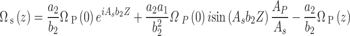
This work studies the generation of the OAM beam in the DQD-MNP under the application of the OAM beam. First, a model is derived for the DQD-MNP system under the OAM applied field and SGC components where the relations for probe and generated fields are attained. Then, these relations are used to study the system properties. Our solution differs from others by the calculated energy states of the DQDs and the computation of the transition momenta between QD-QD and QD-wetting layer (WL) transitions. The orthogonalized plane wave (OPW) is used to calculate QD-WL transitions. It is essential to specify the Rabi frequency of the input field. Note that this work considers both the conduction band (CB) and the valence band (VB) QD and WL states; this is another property of this work. This was not considered earlier in the OAM QD works13, and it is essential for the work to be more realistic. So, the study of the DQD-MNP structure considering the calculation of QD-QD and WL-QD momenta under OPW, which is essential to specify Rabi frequency, characterizes this work from the literature. The way of deriving the relations differs from the literature on OAM in atomic systems. Such characteristics are not used in earlier models. It is vital to make the formulation give a picture of the practice and not use an average value or a value of one structure in another where each structure has its properties that differ from others. This makes the formulation here of material property. SGC is essential in increasing the generated field. The signal field generation in the DQD-MNP system is higher by three orders than in the DQD system alone. So, the DQD-MNP system is preferred to the DQD system. The generated field in the DQD-MNP for the strong coupling case is higher than that for the weak coupling. Increasing the distance separating the DQD-MNP system reduces the generated field. The effect of incoherent pumping is then included, where the density matrix equations system is modified to include such an impact. The results show that the generated field is increased under small incoherent injection. The results of this work make a good comparison to the literature.
DQD-MNP structure
The studied structure is a hybrid DQD-MNP structure. DQDs structure comprises two QDs composed of InAs disk-shaped QDs. These two QDs have 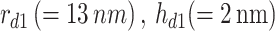 as a radius and height of the first QD, while those of the second QD are
 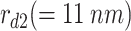 ,
,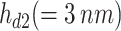 . The MNP is of a spherical shape of
 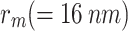 radius. The MNP-DQD distance is denoted by
  ; see Fig. 1. The strong coupling case between the MNP-DQD hybrid system is applied, i.e.,
  17. The WL is an
  quantum well of
  thickness.
Fig. 1.

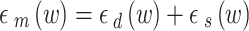
The hybrid WL-DQD-MNP structure. Note that  and
and  are DQD radii,
  is the DQD-MNP separating distance, and
  is the MNP radius.
Modeling
DQD-MNP Hamiltonian
This work considers the DQD-MNP system under the applied probe field 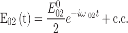 where
where  is the frequency of transition between
  DQD states,
  is the intensity of the applied probe, and
  refers to the complex conjugate. The total Hamiltonian of the system is given by,
 |
1 |
With  is the unperturbed Hamiltonian, which is given by the energy of DQD states
 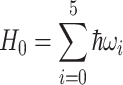 . The relaxation Hamiltonian
  defines the relaxations of the system. The interaction Hamiltonian is given by,
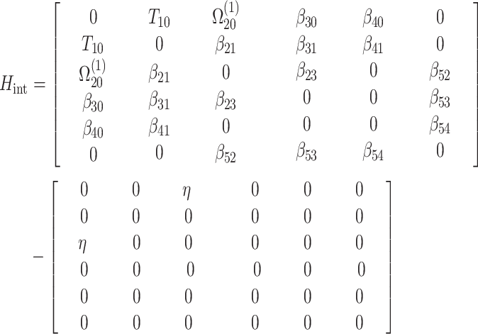 |
2 |
 is the tunneling applied component, and the transition coefficients
  (
( , with
 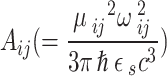 is the Einstein coefficient,
  is the dipole dephasing time,
 is the semiconductor QD dielectric constant,
  is the transition frequency between QD
  and
and  states, and
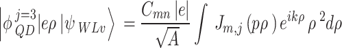
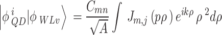
  is the transition momentum, which is here either for QD-QD or WL-QD transition (OPW is used in calculating the latter). The momentum calculation is explained in12.
  is defined after that with the Rabi field.
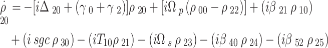
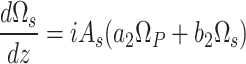
The density matrix equations of the DQD-MNP system
From the density matrix theory, the density operators using the rotating wave approximation for the system in Fig. 2, under the OAM optical probe field  and the generated field
  considering the SGC term, are written as,
Fig. 2.

DQD-MNP system: (a) DQD-MNP under the generated and OAM probe fields, (b) the SGC contribution.
 |
3 |
 |
4 |
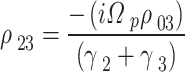
With  is the relaxation from the state
  ,
,  is the detuning under the applied optical probe field,
 is the spontaneously generated coherence. With
  is the relaxation between states
  and
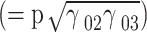
and  . The cross-coupling SGC parameter p is defined by
 |
5 |
This definition is similar to that in the literature15,16.
As long as the only considered fields are  and
and  , the terms in the density matrix with terms containing
  are neglected in
  ,
,  ,
,  . Then, from the density matrix relations, one can use that
 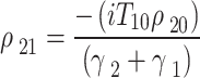 ,
,  ,
,  . Using these relations into
  , gives,
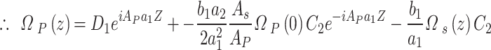
 |
Neglecting the second-order dependence on the applied field. Here,  is small as
  is the weak probe field. Then
  becomes,
 |
6 |
Where 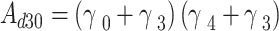 . Also, denote,
  ,
,  =
=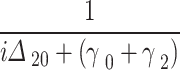 , then,
 |
,
Now, substitute  into
into  relation to get,
 |
Neglecting the last term (taking only the linear dependence on the applied fields. Denote,
 |
The density matrices in Eqs. (1), (2) can be written as,
 |
Or,
 |
7 |
With
 |
8 |
 |
9 |
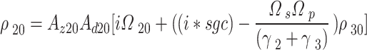
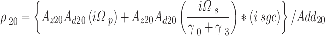
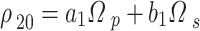
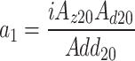
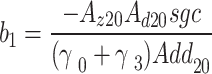
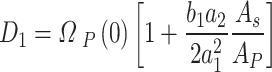
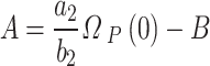
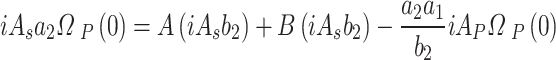
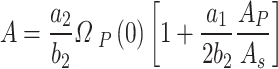
To get the relation of  , denote,
 |
The relation of  can be written as,
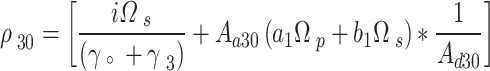 |
Then,
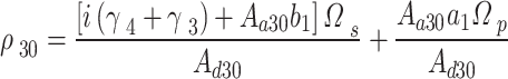 |
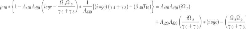
The second relation is
 |
10 |
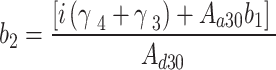 |
11 |
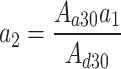 |
12 |
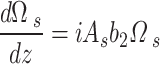
The Rabi fields
The following relations are derived for the generated and probe Rabi fields,
 |
13 |
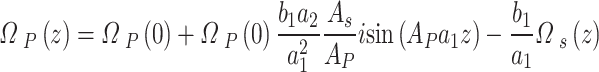 |
14 |
Their derivation is set in Appendix A. Note that the vortex defines the OAM probe optical field is18,
 |
15 |
Where  is the distance from the vortex,
  is the beam waist,
  is the OAM number along the propagation direction and
  is the azimuthal angle. Note that
  is the applied probe field defined as19,
 |
16–a |
The above definition is at strong coupling, and,
 |
16–b |
With the applied probe Rabi frequency19,
 |
16–c |
where  is the momentum of the transition between the states
  ,
,  and
and  is the strength of the probe field applied between these states. The Rabi frequency at weak coupling is defined by
  alone. The calculated momentum
  and also WL-QD momenta is set in the Appendix B, and,
 |
16–d |
Note that  is the electric field direction where
  is for the z-axis polarization and
  is for the parallel direction. The screened dielectric constant in the DQD or the MNP is defined by19,
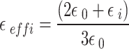 |
16–e |
where  is either
  for the semiconductor DQD or
  for the MNP. Also, define
 |
16–f |
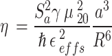
Equation (13) defines the strong coupling11. The dielectric function of the MNP is defined by20,
 |
17–a |
where  represents the contribution of the s-state electrons to the dielectric constant. It is defined in the Drude model by20,
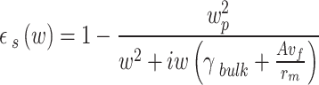 |
17–b |
where  is the damping constant of the bulk metal,
  is the electron velocity at Fermi energy,
  is the plasma frequency of the metal, and
  is related to the MNP electron scattering. In Eq. (14–a),
  is the contribution of the d-state electrons in the MNP. For the gold MNP at the plasma frequency
 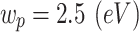 , it defined by20,
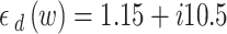 |
17–c |
Using the Drude model in the strong coupling QD-MNP is a common assumption. This results from the high concentration of electrons, as well as in MNP21.
Results and discussion
This work simulates the optical properties of the DQD-MNP structure subjected to a probe optical field with OAM considering SGC in the structure. While the pump and OAM probe field relations are derived analytically, the DQD energy states and the WL-QD and QD-QD transition momenta ( ) are calculated via MAOUD-37 software written under MATLAB12. So, the work here differs from other works regarding material property. Such property comes from calculating QD energy states and momenta for the structure under study. The WL state with WL-QD transition momenta are also calculated in the computation, considering the inevitable OPW between WL and QDs. This is not considered earlier. The parameters used in the calculations are listed in Table 1. The calculated momenta are also listed to make it easy to repeat calculations. Note that the relaxations
  that form the two parts of the SGC, Fig. 2, are taken as
 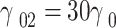 and
and  . Such difference takes into account their difference in energy; in addition, the state
  is in another QD. Then
  , and
, and  are taken and
  . For the WL state, the relaxation is taken at longer time than the QD,
 22. The cross-coupling SGC parameter p values are chosen between
  and
and  as in the literature15,16.
Table 1.
The parameters used in the calculations.
| Parameter | Symbol | Value (unit) | Ref. | |
|---|---|---|---|---|
| The QD relaxation rates |

|

|
22 | |
| The WL relaxation rates |

|

|
22 | |
| Dephasing time |

|

|
23 | |
| InAs QD dielectric constant |

|

|
24 | |
| Damping constant of the bulk metal |

|

|
20 | |
| Electron velocity at Fermi energy |

|
|
20 | |
| Plasma frequency of the metal |

|

|
20 | |
| Tunneling component |

|

|
||
| Input probe frequency (considering screened metal contribution) |

|
|
||
| Calculated QD momenta | ||||
|---|---|---|---|---|
| Momentum | Value (nm.e) | Momentum | Value (nm.e) | |

|
11.2635 |

|
6.2047 | |

|
0.0161 |

|
6.1059 | |

|
0.0055 |

|
1.4652 | |

|
13.4620 |

|
1.3725 | |

|
0.0047 |

|
0.0139 | |
Unless stated otherwise, the following data are used:  ,
,  ,
,  , device length
  , beam wais
  , the distance from the vortex
 , the OAM number along the propagation direction
 =1 and the azimuthal angle
  , and
, and  . Such data are chosen depending on what is used in the literature, such as in18.
Figure 3 shows the field-generated  normalized to the applied probe field
  as a function of the normalized spatial distance
  under three spontaneously generated coherence (SGC) ratios
  . The generated field begins from zero and linearly increases with distance. The highest value of the generated field is
  at
at  . Such limitation of the field generated can be ascribed to the absorption through the system. The generated field ratio increases with SGC, showing the importance of SGC in increasing the generated field. The behavior of increasing the generated field along the device length with SGC has already been demonstrated in other works2,6. SGC adds extra atomic coherence, causing an EIT, increasing the nonlinearity, and reducing absorption. This causes the raising of curves with increasing the SGC parameter (p)16,25.
Fig. 3.

Normalized generated field versus normalized distance at three SGC ratios.
Figure 4 shows the applied probe field ratio  as a function of the normalized spatial distance
  under the SGC ratios
  . The applied field linearly descends due to the absorption through the device. The high SGC ratio reduces the applied field via the generating field. Such behavior is also shown in13.
Fig. 4.

Normalized probe field versus normalized distance at three SGC ratios.
Figure 5 shows the normalized OAM-generated field concerning distance from the vortex  normalized by the beam waist
  at three OAM numbers. Increasing the OAM number amplifies the generated field and shifts the amplified peak to a long vortex distance. The behavior of moving the peak of the generated field is also shown in5. More increments of the OAM number reduce the generated field at long distances, as shown in the black curve.
Fig. 5.

Normalized generated probe field versus normalized distance from the vortex at three OAM numbers.
The main features in the probe and generated fields of the atomic structures under structured light are studied in Figs. 3, 4, 5, and as shown in the above results, the results are not much different from other structures.
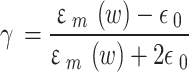
To compare the DQD-MNP structure features with other atomic structures, Fig. 6 is shown. It compares the performance of the DQD-MNP at strong coupling (blue-dotted) with its weak coupling case (red-dashed) and with the DQD (black-dashed curve) systems. Figure 6a compares field generation. For the three systems, the signal field increases with distance. The signal field generation in the DQD-MNP system doubles that of the DQD system alone. Such behavior prefers the DQD-MNP system to the DQD system alone. Figure 6b shows the probe field applied to the systems under study, which is reduced with distance due to the conversion into the generated field.
Fig. 6.

The behavior of the fields along the normalized distance in the DQD-MNP system at strong coupling (blue dotted), DQD-MNP system at weak coupling (red-dotted), and DQD system (black-dotted): (a) normalized generated field. (b) normalized probe field.
Figure 7 compares the coupling cases of the MNP-DQD system, where the strong coupling case 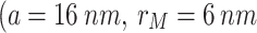 –blue curve) is compared with two weak coupling cases: the red curve
 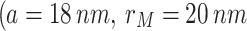 ) and black curve
  . The signal field at the strong coupling is higher by more than one order than the weak cases. Increasing MNP-DQD distance (
 reduces the generated field. Thus, strong coupling is preferred. From Figs. 6, 7, the effect of coupling the MNP to the DQD is evident, where the generated field in the DQD-MNP structure becomes high compared to the DQD structure alone. This can be explained by Eq. (16) above, where parts are added due to the MNP contribution. The QD-MNP system has a strong exciton-plasmon coupling without needing an externally applied pump field or incoherent fields. An energy transfer from the MNP to the QD suggests the generation of quantum coherence in the QD-MNP system26. Such coherence reduces the absorption25 and increases the generated field.
Fig. 7.

The behavior of the generated field along the normalized distance in the DQD-MNP system at strong coupling (blue) and DQD-MNP system at weak coupling (red and black).
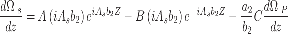
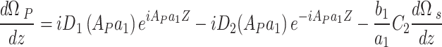
Equations (1), (2) are then modified to include the incoherent pumping term, and the formulation is shown in Appendix C. Figure 8 shows the generated field as a function of the optical depth  at three values of the incoherent pumping
  . It is shown that the incoherent pumping reduces the generated field, a behavior shown in6 for a three-level atomic system.
Fig. 8.

The effect of the optical depth at three incoherent pumpings on the normalized generated field.
Conclusions
An analytical model for the OAM probe field and the generated one in the DQD-MNP system is derived. WL-QD transitions, with OPW, in addition to QD-QD, are considered. SGC is considered. The calculations here are of material property through the computation of the QD-QD and WL-QD transition momenta, which are essential for specifying the Rabi frequency. The results show that SGC increases the generated field. The signal field generation in the DQD-MNP system doubles that from the DQD system alone. So, the DQD-MNP system is preferred to the DQD system. The generated field in the DQD-MNP for the strong coupling case is higher than that for the weak coupling. The strength of the exciton-plasmon coupling depends on the distance separating the strong DQD-MNP structure. At strong coupling (short distances), more energy is transferred from the MNP to the DQD, generating a quantum coherence. This coherence reduces the absorption and increases the generating field. Increasing the DQD-MNP distance reduces the generated field. The model is then extended to include the incoherent pumping, and the relations are modified to include this effect. Small incoherent pumping increases the generated signal. This study compared well with the literature, while those comparing the weak with strong coupling are only done in this work for the first as long as the OAM in the MNP-DQD structure is studied here for the first. The results open the way to study quantum entanglement as quantum coherence increases under SGC. Slow light is also a promising application, as the absorption is reduced with strong coupling.
Acknowledgements
As we noticed that you have used software [MAOUD-37 ] in your study. Kindly provide the following in main manuscript: a. Full name of software and Version numberb. URL linkDear Prof. This software is my own lab software. It is not put in the internet. I use it in a very large number of our papers. one of them is published in the scientific reports. This paper isAkram, H., Abdullah, M. and Al-Khursan, A. H. Energy absorbed from double quantum dot-metal nanoparticle hybrid system. Scientific Reports 12, 21495 (2022).
Appendix A: derivation of optical properties of DQD-MNP with OAM
The following relations are used
 |
A–1 |
With  and
and  is the optical depth of the signal-generated field. Eq. (A–1) is solved by separating its homogenous and particular parts as follows: for the homogenous solution,
 |
A–2a |
Giving,
 |
A–2b |
With  and
and  are constants to be calculated. For the particular solution,
 |
A–3a |
Giving,
 |
A–3b |
With  is a constant to be calculated. Summing homogeneous and the particular solution gives,
 |
A–4 |
Rewrite Eq. (A–1) using Eq. (A–4),
 |
A–5 |
So, one must use the second equation,
 |
A–6 |
With  and
and  is the optical depth of the probe field. Using (A–6) in Eq. (A–5), and using it in Eq. (A–1), gives,
 |
Applying the following conditions
 |
A–7 |
Where the probe field is applied only. This gives,
 |
A–8 |
Now, return to the second equation, Eq. (A–6). In the same way, the complete solution is given as,
 |
A–9 |
and using into (A–6), one obtains,
 |
A–10 |
Using Eq. (A–10) into Eq. (A–6) gives,
 |
Then using Eq. (A–2) in the above relation at  , gives,
 |
Then,
 |
 |
A–11 |
To get  , one must use the particular solution from Eq. (A–9),
 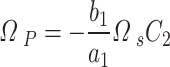 , and substitute it into the particular equation
 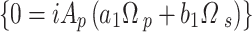 obtained from Eq. (A–6) to get
 |
 |
Substitute into Eq. (A–11) gives,
 |
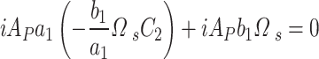
Applying the boundary conditions (A–7) gives,
 |
A–12 |
This returns to
 |
A–13 |
The same way of obtaining  is used to obtain
  where it gives
  . Now, to get the constants
  one must write Eq. (A–4) in the case
 |
 |
A–14 |
From Eq. (A–8), one can write
 |
Using Eq. (A–14) to get,
 |
Which gives,
 |
Giving,
 |
Then,
 |
Results in,
 |
A–15 |
Substitute Eq. (A–13) into (A–15) results in,
 |
Which finally results in
 |
A–16 |
Appendix B: momentum matrix elements
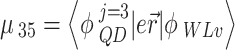
Only two density matrix equations relating to the transitions considered in the SGC appear in this work. Although of this, all the transition momenta are calculated through this work. They are also used in the calculations. Their use is in the calculation of the transition coefficients  (
( , with
  where
where  is the transition momentum between
  and
and  states. Then, one has either QD-QD interdot transitions or WL-QD type depending on the states
  and
and  are for DQD or WL. For the interdot transitions, taking
  momentum as an example12,
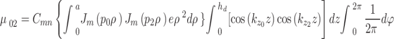 |
B–1 |
In Eq. (B–1),  is the normalization constant for the in-plane QD wavefunction, which is in the form of the Bessel function
  with
with  its variable determined from the interface boundary conditions between the quantum disk and the WL material,
  is the radius of the quantum disk (QD). The wavenumber of the state
  in the z-direction is
 .
.
As an example of the WL-QD transitions, take the transition momentum  in the VB, it is written as12,
 |
B–2 |
 |
B–3 |
There are two parts of integration here. The first is in the in-plane ( ) direction of the quantum disk, and the second ( the cosine-type) is in the z-direction. This form is to cover the overall wavefunctions of the states under calculation.
  is a unit vector in the in-plane direction, the wavefunctions
  ,
,  are for QD state
  and WL VB, in the
  -direction,
  ,
,  are the normalization constants of the wavefunctions in the z-direction, while
  and
and  are the z-direction wavevectors for the QD state
  and WL VB state, respectively. The first integration in Eq. (B–3), which is in the
  -direction, contains the OPW integration. It is written as15,
 |
B–4 |
 is the normalization constant in the OPW, it is defined by15,
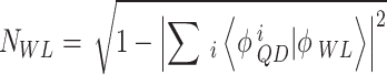 |
B–5 |
The summation runs through all DQD states. Other integrations in Eq. (B–4) are written as15,
 |
B–6 |
 |
B–7 |
 |
B–8 |
A similar integration is also found for the CB.
Appendix C: including incoherent pumping
The density matrix equations of the DQD-MNP under considering an incoherent pumping  reads,
 |
 |
Then,  is introduced into the following variables,
 |
 |
 |
 |
 |
Author contributions
Authors’ contributions: The authors contributed equally.
Data availability
This article includes all the data generated or analyzed during this study.
Declarations
Competing interests
The authors declare no competing interests.
Consent to participate
All the authors consented to participate.
Consent for publication
All the authors consent to publication.
Footnotes
Publisher’s note
Springer Nature remains neutral with regard to jurisdictional claims in published maps and institutional affiliations.
References
- 1.Moretti, D., Felinto, D. & Tabosa, J. W. R. Collapses and revivals of stored orbital angular momentum of light in a cold-atom ensemble. Phys. Rev. A79, 023825 (2009). [Google Scholar]
- 2.Hamedi, H., Reza, Ruseckas, J., Paspalakis, E. & Juzeliunas, G. Transfer of optical vortices in coherently prepared media. Phys. Rev. A99, 033812 (2019). [Google Scholar]
- 3.Asadpour, S. H. et al. Azimuthal modulation of electromagnetically induced grating using structured light. Sci. Rep.11, 20721 (2021). [DOI] [PMC free article] [PubMed] [Google Scholar]
- 4.Wang, T., Zhao, L., Jiang, L. & Yelin, S. F. Diffusion-induced decoherence of stored optical vortices. Phys. Rev. A77, 043815 (2008). [Google Scholar]
- 5.Hamedi, H., Reza, Ruseckas, J. & Juzeliunas, G. Exchange of optical vortices using an electromagnetically-induced-transparency–based four-wave-mixing setup. Phys. Rev. A98, 013840 (2018). [Google Scholar]
- 6.Asadpour, S. H., Ziauddin, Abbas, M. & Hamedi, H. R. Exchange of orbital angular momentum of light via noise-induced coherence. Phys. Rev. A105, 033709 (2022). [Google Scholar]
- 7.Jia, N., Qian, J., Kirova, T., Juzeliunas, G. & Hamedi, H. R. Ultraprecise Rydberg atomic localization using optical vortices. Opt. Express28, 36936–36952 (2020). [DOI] [PubMed] [Google Scholar]
- 8.Wu, S. et al. Generation of dual-polarization orbital angular momentum vortex beams with reflection-type metasurface. Opt. Commun.553, 130107 (2024). [Google Scholar]
- 9.Wu, W., Wang, Z., Huang, Z. & Yu, B. On-off switching of orbital-angular-momentum light via atomic collision. Opt. Laser Technol.175, 110872 (2024). [Google Scholar]
- 10.Liu, S., Lou, Y. & Jing, J. Orbital angular momentum multiplexed deterministic all-optical quantum teleportation. Nat. Commun.11, 3875 (2020). [DOI] [PMC free article] [PubMed] [Google Scholar]
- 11.Hameed, A. H. & Al-Khursan, A. H. Tunability of plasmonic electromagnetically induced transparency from double quantum dot-metal nanoparticle structure under transition momenta. Opt. Quant. Electron.55, 1213 (2023). [Google Scholar]
- 12.Akram, H., Abdullah, M. & Al-Khursan, A. H. Energy absorbed from double quantum dot-metal nanoparticle hybrid system. Sci. Rep.12, 21495 (2022). [DOI] [PMC free article] [PubMed] [Google Scholar]
- 13.Mahdavi, M., Sabegh, Z. A. & Mohammadi, M. Manipulation and exchange of light with orbital angular momentum in quantum-dot molecules. Phys. Rev. A101, 063811 (2020). [Google Scholar]
- 14.Niu, Y., Gong, S., Li, R. & Jin, S. Creation of atomic coherent superposition states via the technique of stimulated Raman adiabatic passage using a L-type system with a manifold of levels. Phys. Rev. A70, 023805 (2004). [Google Scholar]
- 15.Al-Salihi, F. R. & Al-Khursan, A. H. Electromagnetically induced grating in double quantum dot system using spontaneously generated coherence. Chin. J. Phys.70, 140–150 (2021). [Google Scholar]
- 16.Bai, Y., Liu, T. & Yu, X. Giant Kerr nonlinearity in an open V-type system with spontaneously generated coherence. Optik124, 613–616 (2013). [Google Scholar]
- 17.Yan, J. Y., Zhang, W., Duan, S., Zhao, X. G. & Govorov, A. O. Optical properties of coupled metal-semiconductor and metal-molecule nanocrystal complexes: role of multipole effects. Phys. Rev. B77, 165301 (2008). [Google Scholar]
- 18.Hamedi, H., Reza, Paspalakis, E., Žlabys, G., Juzeliunas, G. & Ruseckas, J. Complete energy conversion between light beams carrying orbital angular momentum using coherent population trapping for a coherently driven double- atom-light-coupling scheme. Phys. Rev. A100, 023811 (2019). [Google Scholar]
- 19.Sadeghi, S. M., Deng, L., Li, X. & Huang, W. P. Plasmonic (thermal) electromagnetically induced transparency in metallic nanoparticle–quantum dot hybrid systems. Nanotechnology20, 365401 (2009). [DOI] [PubMed] [Google Scholar]
- 20.Hatef, A., Sadeghi, S. M. & Singh, M. R. Plasmonic electromagnetically induced transparency in metallic nanoparticle–quantum dot hybrid systems. Nanotechnology23, 065701 (2012). [DOI] [PubMed] [Google Scholar]
- 21.Hakami, J. & Zubairy, M. S. Nanoshell-mediated robust entanglement between coupled quantum dots. Phys. Rev. A93, 022320 (2016). [Google Scholar]
- 22.Ben Ezra, Y., Lembrikov, B. I. & Haridim, M. Specific features of XGM in QD-SOA. IEEE J. Quantum Electron.43, 730–737 (2007). [Google Scholar]
- 23.Sridharan, D. & Waks, E. All-optical switch using quantum-dot saturable absorbers in a DBR microcavity. IEEE J. Quantum Electron.47, 31–39 (2011). [Google Scholar]
- 24.Chuang, S. L. Physics of Optoelectronic Devices (Wiley, 1995).
- 25.Al-Nashy, B., Razzaghi, S., Al-Musawi, M. A., Saghai, H. R. & Al-Khursan, A. H. Giant gain from spontaneously generated coherence in Y-type double quantum dot structure. Res. Phys.7, 2411–2416 (2017). [Google Scholar]
- 26.Kosionis, S. G., Terzis, A. F., Sadeghi, S. M. & Paspalakis, E. Optical response of a quantum dot-metal nanoparticle hybrid interacting with a weak probe field. J. Phys. Condens. Matter25, 045304 (2013). [DOI] [PubMed] [Google Scholar]
Associated Data
This section collects any data citations, data availability statements, or supplementary materials included in this article.
Data Availability Statement
This article includes all the data generated or analyzed during this study.