A Statistical Characterization of Dynamic Brain Functional Connectivity

ABSTRACT

This study examined the statistical underpinnings of dynamic functional connectivity in mental disorders, using resting‐state fMRI signals. Notably, there has been an absence of research demonstrating the non‐stationarity of the empirical probability distribution of functional connectivity. This gap has prompted debate on the existence of dynamic functional connectivity, leading skeptics to question its relevance and the reliability of research findings. Our aim was to fill this gap by conducting a comprehensive empirical distribution analysis of functional connectivity, using Pearson's correlation as a measure. We conducted our analysis on a set of preprocessed resting‐state fMRI samples obtained from 186 subjects selected from the UCLA Consortium for Neuropsychiatric Phenomics dataset. Departing from conventional methods that aggregated signals over voxels within a region of interest, our approach leveraged individual voxel signals. Specifically, our approach offered a precise characterization of the empirical probability distribution of resting‐state fMRI signals by evaluating the temporal variations and non‐stationarity in dynamic functional connectivity, as measured by Pearson's correlation. Our study investigated functional connectivity patterns across 49 regions of interest, comparing healthy control subjects with patients diagnosed with ADHD, bipolar disorder, and schizophrenia. Our analysis revealed that (1) the empirical distribution of the correlation coefficient exhibited non‐stationarity, (2) the beta distribution was an accurate approximation of the exact correlation coefficient distribution, and (3) the empirical distribution of means derived from the fitted beta distributions, unraveled distinctive dynamic functional connectivity patterns with potential as biomarkers associated with different mental disorders. A key contribution of our study was the presentation of the first comprehensive empirical distribution analysis of dynamic functional connectivity, thus providing compelling evidence for its existence. Overall, our study presented an innovative statistical approach that advances our understanding of the dynamic nature of functional connectivity patterns derived from resting‐state fMRI. Our examination of the empirical distribution of dynamic functional connectivity provided solid evidence supporting its existence. The distinctive dynamic functional connectivity patterns we identified across various mental disorders hold promise as potential biomarkers for further development.

To our knowledge, this study represents the first demonstration of non‐stationarity within the empirical probability distribution of functional connectivity, measured by Pearson's correlation of fMRI signals. Our analysis utilized individual voxel signals instead of aggregated signals, providing a precise characterization of the empirical probability distribution of resting‐state fMRI signals.

Summary.

• The brain mapping literature continues to debate the existence of dynamic functional connectivity, leading to skepticism regarding its relevance and the reliability of research findings. To our knowledge, this is the first study that demonstrated non‐stationarity within the empirical probability distribution of functional connectivity, measured by Pearson's correlation of fMRI signals.

• Our examination of the empirical distribution of dynamic functional connectivity provided solid evidence supporting its existence. This finding resulted from our unique approach, which leveraged individual voxel signals, allowing accurate characterization of the empirical distribution and assessment of its temporal variations.

• By conducting a comparative assessment of the empirical distributions from brain regions between healthy controls and patients, we discerned distinctive dynamic functional connectivity patterns associated with various mental disorders.

1. Introduction

The human brain, with its intricate and dynamic nature, comprises numerous interacting regions, presenting a longstanding challenge in understanding their connectivity and collective functioning (Bear, Connors, and Paradiso 2020). The advent of functional magnetic resonance imaging (fMRI) has revolutionized our ability to non‐invasively gather extensive data on brain activity, both in healthy individuals, and those with various mental disorders (Wager and Lindquist 2015). Through fMRI, the measurement of the Blood Oxygen Level‐Dependent (BOLD) signal serves as a valuable proxy for brain activity, enabling the capture of neuronal dynamics throughout the entire brain. This method boasts an impressive spatial resolution at the millimeter level, effectively dividing the brain volume into thousands of voxels, measured with a temporal resolution of 1–3 s, thereby offering a detailed depiction of the functional dynamics of the brain (Chang and Glover 2010; Leonardi et al. 2013).

The investigation into the interactions and interconnectedness of different brain regions during the execution of a given task initially focused on static functional connectivity (sFC) (Biswal et al. 1995; Thomas Yeo et al. 2011; Yeo et al. 2014). sFC examines the synchronization of neural activity between various brain regions, disregarding any variation in temporal information. The conventional method of measuring sFC begins with extracting the signal time series from a specific brain region of interest (ROI), involving the computation of average BOLD signals from all individual voxels within that ROI. Pearson's correlation of the signal time series between two regions, measuring the linear relationship, is commonly used as a sFC metric (Power et al. 2011). This correlation coefficient serves as an indicator of the strength of functional connectivity between the two regions. Additionally, some studies have utilized alternative measures such as partial correlation (Fransson and Marrelec 2008) or mutual information (Chai et al. 2009) to assess sFC.

Rather than being static, functional connectivity is recognized as dynamic and subject to variation over time (Chang and Glover 2010), a concept known as dynamic functional connectivity (dFC) (Preti, Bolton, and Van De Ville 2017). To capture dFC, researchers commonly calculate the fluctuation in the correlation coefficient of signal time series between two brain regions across time. This is achieved by employing a sliding window of a predetermined shape and size (Allen et al. 2014; Damaraju et al. 2014; Mokhtari et al. 2019), though alternative approaches have also been proposed (Karahanoğlu and Van De Ville 2015; Savva, Mitsis, and Matsopoulos 2019; Shine et al. 2015). After evaluating dFC between individual brain regions, researchers can examine the temporal change in patterns of dFC across the whole brain. This holistic approach facilitates a thorough exploration of how dFC evolves over time throughout the entire brain. The correlation matrix of the signal time series from all brain regions is frequently referred to as the dFC pattern of the brain at a specific point in time (Spencer and Goodfellow 2022). Various studies showed temporal changes in the dFC pattern, even during rest periods when the brain was not engaged in any specific task (Liu et al. 2019). The effectiveness of these temporal changes in the dFC pattern in differentiating between healthy individuals and patients with different mental disorders has also been studied (Damaraju et al. 2014; Rashid et al. 2016).

However, the analysis methods applied to dFC have sparked some controversy. While some studies demonstrated dFC through the temporal variability of functional connectivity, typically measured by metrics like Pearson's coefficient (Chang and Glover 2010), others argued that the evidence remained insufficient. This is because temporal variability is inherently present in any random process, even if that process is stationary with unchanged underlying characteristics (Liégeois et al. 2017). Put another way, if we consider the functional connectivity of fMRI signals, measured by the correlation coefficient, as a random process adhering to a specific probability distribution, observing significant temporal variability over time could be a chance occurrence. This might happen while the underlying probability distribution remains unchanged. Some previous studies incorrectly assumed that non‐weak‐sense stationarity observed in a few signal time series would imply dFC, which is invalid (Allen et al. 2014). To compellingly establish that a random process is variant over time, it is essential to gather sufficient realizations to accurately capture the nuanced temporal variations within the empirical probability distribution.

Indeed, there is a lack of research demonstrating dFC by showcasing the non‐stationarity of the empirical probability distribution of functional connectivity, measured by Pearson's correlation, in fMRI signals (Lurie et al. 2020). Consequently, there is a compelling argument that previous findings reported on dFC might be associated with observing random fluctuations inherent to an underlying stationary random process, rather than reflecting genuine dFC (Liégeois et al. 2017; Lurie et al. 2020). This gap in our understanding of dFG emphasizes the need for a comprehensive examination of the statistical underpinnings of dFC.

In this study, we aimed to fill this crucial research gap by adopting a distinctive approach to explore brain functional connectivity patterns. Our specific focus was on examining the empirical probability distribution of functional connectivity, measured by Pearson's correlation. We conducted our analysis on a set of preprocessed resting‐state fMRI (rs‐fMRI) samples obtained from 186 subjects selected from the UCLA Consortium for Neuropsychiatric Phenomics dataset (Gorgolewski, Durnez, and Poldrack 2017). In contrast to the conventional method of averaging signals from voxels within a given ROI, our study took advantage of the inherent fluctuations in signal time series across multiple individual voxels. We assumed that the proximate individual voxel time series were realizations of an identical underlying random process within a specific ROI. This unique approach provided us with access to a diverse array of realizations, facilitating precise characterization of the empirical probability distribution and allowing the assessment of its temporal variations and non‐stationarity. Our results contributed robust evidence of dFC by demonstrating that the empirical distribution of correlation coefficients between two regions exhibited non‐stationarity when observed across different time shifts.

Building on our approach of modeling the empirical distribution of correlation coefficients between two regions, we extended our investigation to explore the impact of mental disorders on dFC. What distinguished this analysis was our unique statistical approach, which involved computing the empirical distribution of means derived from the fitted distributions of correlation coefficients between two regions across a group of subjects. Subsequently, the identified empirical distribution of means served as the dFC pattern. Our analysis included a comparative study of brain dFC patterns across a comprehensive set of 49 ROIs. Specifically, we compared these dFC patterns between healthy control (HC) subjects (48 subjects) and each group of patients diagnosed with ADHD (41 subjects), bipolar disorder (BP) (48 subjects), and schizophrenia (SZ) (49 subjects). Notably, we discerned distinctive dFC patterns associated with various mental disorders based on the empirical distribution analysis.

2. Materials and Methods

2.1. Data Acquisition

The preprocessed resting state fMRI (rs‐fMRI) dataset from the UCLA Consortium for Neuropsychiatric Phenomics (CNP) dataset (Gorgolewski, Durnez, and Poldrack 2017) was included in this study. The dataset contained healthy controls (HC) (130 subjects), as well as participants with adult attention‐deficit hyperactivity disorder (ADHD) (42 subjects), bipolar disorder (BP) (49 subjects) and schizophrenia (SZ) (50 subjects). The rs‐fMRI dataset was collected from participants who underwent a rs‐fMRI session lasting 304 s while keeping their eyes open. Spatial smoothing was applied using AFNI's 3dBlurInMask with a Gaussian kernel with FWHM = 5 mm. The repetition time (TR) is 2000 ms. The first 48 HC subjects based on their subject ID, out of a total of 130 HC subjects, were selected for analysis. One ADHD subject and one BP subject were excluded from the analysis due to the inability to successfully extract all voxel signals from these individuals. In summary, a more balanced dataset of 48 HC subjects, 41 ADHD subjects, 48 BP subjects, and 49 SZ subjects were studied and compared. The demographic information of the dataset studied is shown in Table 1.

TABLE 1.

Demographic information of the dataset studied from UCLA CNP.

	HC	ADHD	BP	SZ
Number of subjects	48	41	48	49
Gender (m/F)	26 M, 22 F	20 M, 21 F	27 M, 21 F	38 M, 11 F
Ages	21–49	21–50	21–50	22–49

2.2. Data Preprocessing

Spatial normalization was first applied to the preprocessed rs‐fMRI images from the UCLA CNP dataset. All the images were registered to a standard MNI brain template, resampled to 1 mm × 1 mm × 1 mm to ensure an adequate sample size, using the ANTs neuroimage processing library (Stnava 2023). The brain atlas by Seitzman et al. (2020) was then used to parcellate the brain into 49 regions of interest (ROIs). The brain atlas was generated from eyes‐open resting‐state fMRI data, thus it was well‐suited for the purpose of this study. The 49 subcortical and cerebellar ROIs were part of four networks, namely, the Default Mode network (DMN), Cingulo‐Opercular network (CON), Somatomotor Dorsal network (SDN), and Frontoparietal network (FPN). Our rationale for selecting regions in the cerebellum and other subcortical structures was threefold: (1) these regions were not widely studied in previous rs‐fMRI studies compared to cortical regions, and (2) they were more consistent across subjects, both anatomically and functionally, than cortical regions, and (3) they were relatively homogenous over the typical ROI size of 4 mm‐radius spheres. The information on the ROIs and networks from the brain atlas is shown in Table 2.

TABLE 2.

Information of the ROIs and networks from the brain atlas by Seitzman et al. (2020).

	DMN	CON	SDN	FPN	Total
Numbers of ROIs	12	7	21	9	49
REGION:	Cerebellum:	Cerebellum:	Cerebellum:	Cerebellum:
ROI ID: MNI	0: (32, −81, −38)	12: (44, −60, −30)	19: (−6, −74, −42)	40: (−10, −78, −28)
	1: (−32, −78, −38)	13: (−44, −60, −30)	20: (8, −72, −39)	41: (10, −78, −28)
	2: (−24, −76, −28)	14: (−34, −42, −44)	21: (−10, −62, −18)	42: (−34, −72, −48)
	3: (24, −76, −28)	Thalamus:	22: (10, −62, −18)	43: (34, −72, −48)
	4: (−6, −51, −41)	15: (−15, −14, 12)	23: (−33, −51, −50)	44: (−31, −66, −30)
	5: (8, −50, −40)	16: (13, −14, 12)	24: (−12, −44, −18)	45: (32, −63, −30)
	Hippocampus:	17: (−9, −10, 0)	25: (12, −44, −18)	46: (40, −44, −38)
	6: (−25, −39, −2)	18: (10, −8, 2)	Thalamus:	Basal Ganglia:
	7: (25, −37, −2)		26: (−19, −23, 10)	47: (−15, −2, 19)
	Thalamus:		27: (16, −22, 9)	48: (14, −1, 18)
	8: (−5, −10, 9)		28: (−14, −20, 1)
	9: (4, −8, 8)		29: (14, −19, 0)
	Basal Ganglia:		Basal Ganglia:
	10: (−13, 17, 7)		30: (−28, −10, −4)
	11: (12, 18, 7)		31: (−28, −10, 9)
			32: (29, −8, 8)
			33: (28, −7, −5)
			34: (−19, −5, −3)
			35: (19, −5, −4)
			36: (−28, −1, −3)
			37: (25, 2, −1)
			38: (25, 5, 7)
			39: (−25, 8, 8)

Each ROI was defined by its MNI coordinate on the brain map. To extract the time series signals from the ROIs, a 4 mm radius sphere was centered at the MNI coordinate of each ROI, and the time series signals of all the voxels within the sphere were then extracted. The sphere of each ROI comprised 257 voxels.

2.3. BOLD Time Series

The signal time series extracted from the voxels of each ROI were BOLD signals. A signal time series consisting of 152 time points was extracted from each voxel.

2.4. Sliding‐Window Correlations

The Pearson's correlation coefficient was employed as a measure of dFC between two ROIs. To capture the time‐variability of dFC, the Pearson's correlation coefficients were computed over a sliding window of three sizes: 15, 25, and 35 (eq. to 30, 50, and 70 s durations). The sliding window moved with a step size of one (2 s). The smaller window size was beneficial for detecting rapid changes, while a larger window size helped reduce noise and yield a more robust and smoother analysis (Ahrends and Vidaurre 2023). The sliding‐window correlations obtained with a window size of 15 display more pronounced and swift fluctuations. Using a window size of 25, the rapid fluctuations were smoothed out, unveiling a clearer depiction of the overall trend. Further increasing the window size to 35 resulted in even smoother sliding‐window correlations, displaying the comparable trend observed with the smaller window sizes. As the three windows provided very similar results, the window size was set to 35 points (i.e., 70 s) for all analyses (see Supporting Information for additional details).

2.5. Regions of Interest

Each ROI was defined by its MNI coordinate. To capture the temporal dynamics within these ROIs, we defined each ROI as a 4 mm‐radius sphere centered at its MNI coordinate (following the same method as in Seitzman et al. (2020)). Subsequently, we extracted the time series signals from all the voxels located within this sphere. Notably, each sphere, corresponding to an ROI, encompassed a total of 257 proximate voxels.

2.6. Signal Time Series as Random Processes

Our analysis operated on the assumption that the signal time series of the voxels from each ROI originated from an intrinsic random process. Specifically, we postulated that each individual voxel within a given ROI represented a realization of the same underlying random process that characterized the entire ROI. Indeed, due to the well‐documented inherent spatiotemporal correlations in fMRI data with BOLD contrast, voxels' time series within functionally homogenous brain regions would reflect similar functional dynamics mixed with noise. Therefore, it is reasonable to consider each voxel's time series as a realization of the same process in a given ROI (Poldrack 2007), an assumption that is typically assumed when users summarize all voxels' time series into one single representative time series (Tong et al. 2016). Given the close proximity of voxels within an ROI, confined within a 4 mm radius sphere, it is reasonable to infer that they exhibited closely aligned behaviors.

3. Results

3.1. Empirical Probability Distribution of Signals

When examining the signal time series obtained from a specific subject, at each specific time point, we had 257 individual sample signals derived from the 257 voxels within a single ROI. Leveraging the specific data points from these individual voxels, we constructed a histogram, effectively illustrating the empirical distribution of the voxel signals within a specific ROI at a given time instance. In Figure 1, histograms depict the signals of the voxels within different ROIs at time points, 10, 50, and 100 from different subjects. A noteworthy observation was that the distribution of voxel signals at these different time points appeared to closely approximate a normal distribution. The normality of the sample signal distributions was an important consideration as it formed the basis for approximately modeling the empirical probability distribution in subsequent analyses.

FIGURE 1.

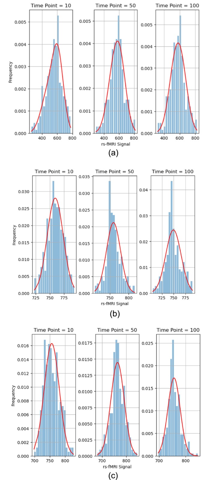
Signals of the 257 voxels within different ROIs at time points, 10, 50, and 100 from different subjects, fitted with a simple normal model (solid red line). (a) One healthy control (HC subject ID 10159) within a Thalamus ROI. (b) One schizophrenia subject (SZ subject ID 50007) within a Basal Ganglia ROI. (c) One ADHD subject (ADHD subject ID 70040) within a Cerebellum ROI.

3.2. Normality of Signals

To validate the normality of the signals of the voxels within a specific ROI, we employed the QQ‐plot. Analyzing the QQ‐plots for the ROIs at time points 10, 50, and 100 from the different subjects, we observed that the majority of sample signals closely align with the 45° reference line, as expected from the good fit demonstrated in Figure 1. This alignment indicated a strong resemblance to a normal distribution, implying that the voxel signals within the different ROIs could be considered approximately normal at different time points. Figure 2 shows QQ‐plots of the 257 voxels within a Thalamus ROI at the time points, 10, 50, and 100, based on data from the HC subject 10,159.

FIGURE 2.

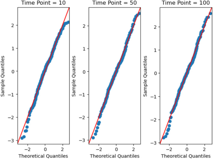
QQ‐plots of the 257 voxels within Thalamus ROI 8 at the time points, 10, 50, and 100 for one healthy control subject (HC subject 10,159).

3.3. Sliding‐Window Correlations

Pearson's correlation coefficient was then employed as a measure of dFC between two signal time series from two ROIs. With a total of 49 ROIs, this led to a comprehensive set of 1176 pairs of ROIs for analysis. Each ROI, characterized by a sphere containing 257 voxels, contributed to the generation of a complete set of 257 × 257 = 66,049 pairs of voxels between each pair of ROIs. While analyzing all 66,049 voxel pairs offers a detailed representation of the underlying distribution, it also requires substantial computational resources. In cases where capturing distribution statistics does not require the full dataset, using a smaller sample (e.g., 257 voxel pairs) can provide a computationally efficient alternative without significant loss of accuracy.

To calculate sliding‐window correlations for a voxel pair within an ROI pair, we first computed the correlation coefficient from the signal time series of that voxel pair within a window of size 35. We then shifted the window was one time point, and repeated the calculation until the end of the time series was reached. Using this approach, a collective count of 118 sliding‐window correlation coefficients was generated over time for each voxel pair within an ROI pair.

3.4. Empirical Probability Distribution of Correlations

Similar to the voxel signals, we could then construct a histogram to show the empirical distribution of the correlation coefficients at a given time point. Figure 3 shows the histograms of correlation coefficients from all the voxel pairs, with n = 257 × 257 samples, between two ROIs at time points, 10, 50, and 100 from different subjects. Importantly, the histograms illustrate shifts and variations in the underlying probability distribution over time.

FIGURE 3.

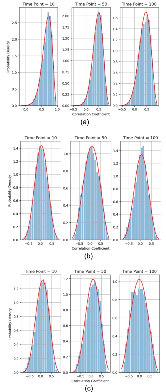
Histograms of correlation coefficients from the voxel pairs between two ROIs at time points, 10, 50, and 100 from different subjects overlaid with the fitted beta distribution approximation (solid red line). (a) One healthy control (HC subject ID 10159) between Thalamus ROI 8 and ROI 9. (b) One schizophrenia subject (SZ subject ID 50007) between Basal Ganglia ROI 38 and ROI 39. (c) One ADHD subject (ADHD subject ID 70040) between Cerebellum ROI 19 and ROI 20.

3.5. Theoretical Probability Distribution of Correlations

Theoretically, if the voxel signals within a specific ROI follow a normal distribution and the signals of voxel pairs connecting two ROIs are bivariate normally distributed, then the sample correlation coefficients derived from these voxel pairs would exhibit a distribution with the probability density function (PDF) given by Equation (1) (Kenney and Keeping 1957):

$$f\left(r\right)=\frac{\left(n-2\right)\mathrm{\Gamma }\left(n-1\right){\left(1-{\rho }^2\right)}^{\frac{n-1}{2}}{\left(1-r^2\right)}^{\frac{n-4}{2}}}{\sqrt{2\pi }\mathrm{\Gamma }\left(\mathrm{n}-\frac{1}{2}\right){\left(1-\mathit{\rho r}\right)}^{n-\frac{3}{2}}}{}_2{}^{}F_1\left(\frac{1}{2},\frac{1}{2};\frac{1}{2}\left(2n-1\right);\frac{1}{2}\left(\mathit{\rho r}+1\right)\right)$$ (1)

where n is the number of sample correlation coefficients, r is the sample correlation coefficient, ρ is the correlation coefficient, Γ is the gamma function, and ₂ F ₁ is the Gaussian hypergeometric function.

3.6. Beta Distribution Approximation of Correlations

It was noted that in a special case when the correlation coefficient is ρ = 0, the distribution of the sample correlation coefficient follows a beta distribution on the interval [−1, 1], with equal shape parameters α = β = n/2–1. The PDF of this beta distribution is derived as Equation (2) (Anderson 2003):

$$f\left(r\right)=\frac{{\left(1-r^2\right)}^{\frac{n-4}{2}}}{B\left(\frac{1}{2},\frac{1}{2}\left(n-2\right)\right)}$$ (2)

where n is the number of sample correlation coefficients, r is the sample correlation coefficient, and B is the beta function.

Building upon the insights from this special case, we further assessed whether the distribution of the sample correlation coefficient could be well approximated by a beta distribution on the interval [−1, 1] when the correlation coefficient deviated from ρ = 0. Numerical simulation was employed to model and simulated the distribution of the sample correlation coefficient. The results of the simulation demonstrated that the distribution of the sample correlation coefficient could be well approximated by a beta distribution on the interval [−1, 1] with the shape parameters α = (n/2–1)/(1—ρ), β = (n/2–1)/(1 + ρ). The PDF of this beta distribution was derived as Equation (3):

$$f\left(r\right)=\frac{{\left(1+r\right)}^{\alpha -1}{\left(1-r\right)}^{\beta -1}}{2^{\alpha +\beta -1}B\left(\alpha ,\beta \right)}$$ (3)

It is worth noting that this beta distribution is the exact distribution of the sample correlation coefficient when the correlation coefficient is ρ = 0.

When n = 257, the PDFs of the sample correlation coefficient and the approximated beta distribution were almost identical. To quantitatively assess the degree of fitness of the PDF of the two distributions, we used the Kullback Leibler Divergence (KLD) as a measure of dissimilarity between the two distributions over the range of ρ values, which spans [−1, 1]. The KLD, also known as relative entropy, measures how much information is lost when one probability distribution is used to approximate another.

Figure 4 shows the KLD between the two distributions when n = 257. As expected, the KLD is 0 when ρ = 0, indicating that the two distributions are the same. When ρ deviates from 0 and increases toward 0.8, the KLD also increases from 0 to 0.0012. The fact that the KLD remains relatively small demonstrates that the approximated beta distribution remains a satisfactory model for the sample correlation coefficient distribution even as the correlation coefficient moves away from 0. Additionally, it was observed that the KLD diminishes with increasing n; for n = 257 × 257, the KLD became too small and close to zero to be calculated with numerical precision. As a result, for the purpose of model fitting, the beta distribution can generally serve as a reliable approximation for the exact PDF of the sample correlation coefficient, especially for sufficiently large n, as in our study.

FIGURE 4.

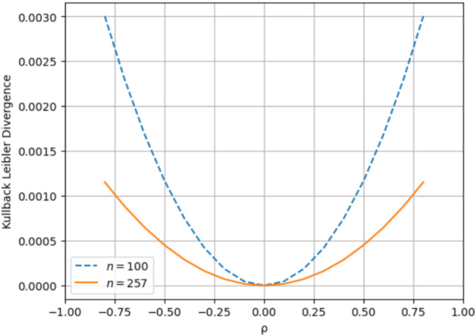
Kullback Leibler Divergence between the exact distribution of the sample correlation coefficient and the approximated Beta distribution over the range of ρ values [−1,1] when n = 100 and n = 257.

It is worth noting that a common approach to avoid working with the exact distribution of the sample correlation coefficient is to use Fisher's z‐transformation, which transforms the correlation coefficient into an approximately normal distribution. One key advantage of this transformation is that it stabilizes the variance of the sample correlation coefficient, making later analysis simpler and more consistent, but see Thompson and Fransson (2016). However, when it is important to demonstrate the non‐stationarity of the correlation coefficient distribution over time, as in this study, working directly with the exact distribution can be more insightful. This approach allows for a clearer observation of how the distribution, including its variance, changes over time.

Additionally, our analysis revealed that the approximated beta distribution is a more accurate approximation than the Fisher's z‐transformed normal distribution for all values of ρ when n = 100 and n = 257. Figure 5 displays the KLD between the distribution of the sample correlation coefficient and the Fisher's z‐transformed normal distribution for both sample sizes. Specifically, when n = 257 and ρ = 0.8, the Fisher's z‐transformed normal distribution yielded a KLD of 11.96, while the approximated beta distribution achieved a KLD of 0.0012. Notably, unlike the beta approximation, the KLD for the Fisher's z‐transformed normal distribution was not zero when ρ = 0, staying at 0.0000269. Additionally, for small values of ρ (e.g., ρ = 0.2), the KLD for the Fisher's z‐transformed normal distribution decreases as n increases from 100 to 257. In contrast, for larger values of ρ (e.g., ρ = 0.8), the KLD for the Fisher's z‐transformed normal distribution is higher when n = 257, while the KLD for the beta approximation continues to decrease as n grows. When ρ is near −1 or 1, the distribution of the sample correlation coefficient becomes highly skewed and tightly bound within the range of −1 and 1. Fisher's transformation stretches this bounded range into an unbounded one, resulting in increasingly extreme values near the boundaries. Although Fisher's transformation was designed to approximate normality for moderate values of ρ, it becomes less accurate at these extremes (Chaubey and Mudholkar 1978). Further details are available in the Supporting Information.

FIGURE 5.

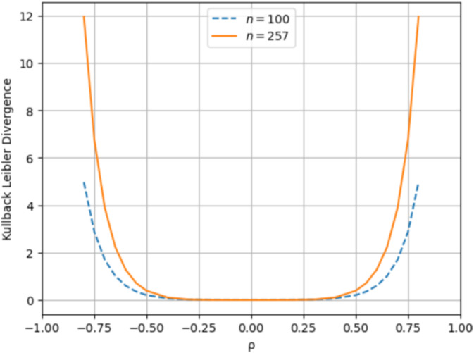
Kullback Leibler Divergence between the exact distribution of the sample correlation coefficient and the Fisher's z‐transformed normal distribution over the range of ρ values [−1, 1] when n = 100 and n = 257.

3.7. Non‐Stationary of Correlation Coefficient Distribution Over Time

To provide empirical validation for the existence of dFC, it was necessary to demonstrate the non‐stationary of the correlation coefficient distribution of the signals from voxel pairs between 2 ROIs across time. The two‐sample Kolmogorov–Smirnov (KS) test is a non‐parametric statistical test that allows us to determine whether two samples are drawn from the same population or from different populations with different underlying distributions. Using the two‐sample KS test, we could investigate whether the correlation coefficient samples from the voxel pairs between the 2 ROIs, obtained from time points 10, 50, and 100, essentially originated from the same distribution as the samples taken at all other time points. This investigation shed light on the stationarity of the underlying distribution across different time instances.

The results of the two‐sample KS test are shown in Figure 6. Given the often‐minuscule p‐values resulting from the KS test, we transformed these values using the –log ₁₀ function (capped at a maximum value of 300) to enhance clarity and interpretation. To adjust for multiple comparisons, we applied Bonferroni correction, setting the significance level at approximately 0.0004 (0.05 divided by 118). The p‐values smaller than or equal to 0.0004 (corresponding to –log ₁₀ p‐value ≥ 3.4), visually represented in red, indicate that the two correlation coefficient samples from the two different time points were improbable to stem from the same distribution. Conversely, p‐values larger than 0.0004 (−log ₁₀ p‐value < 3.4), depicted in blue, suggest that the two correlation coefficient samples were likely drawn from the same distribution. As the figures show, the correlation coefficient samples originating from temporally distant time points generally exhibited significant statistical dissimilarity when compared to the samples extracted from time points 10, 50, and 100, underscoring the non‐stationarity in the correlation coefficient distribution across different time instances.

FIGURE 6.

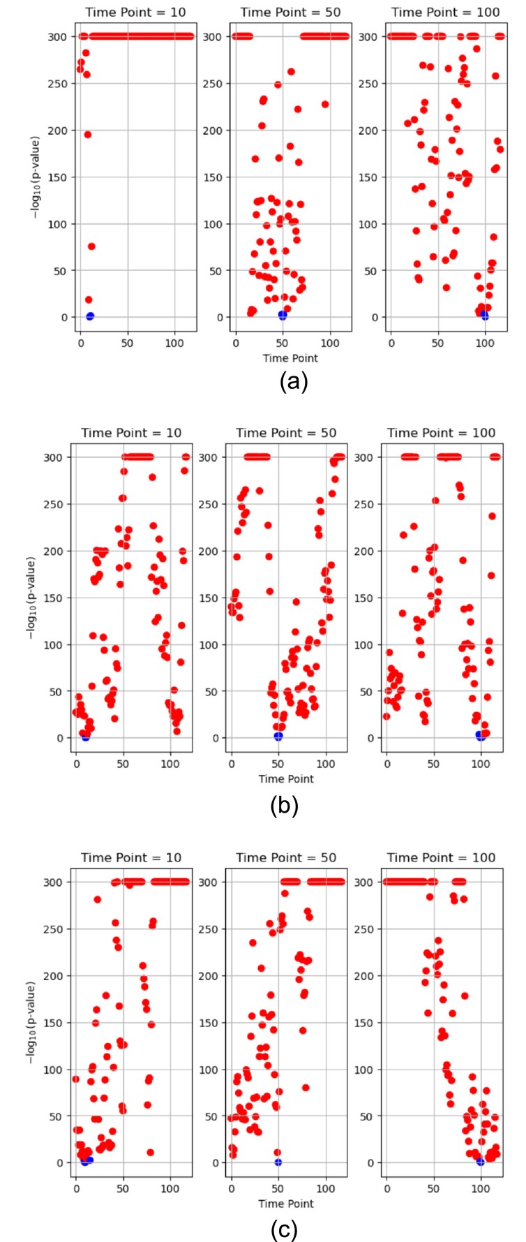
Results of the two‐sample Kolmogorov–Smirnov test conducted on the correlation coefficient samples from two ROIs of different subjects between specific time points (at 10, 50, and 100) and all other time points (−log ₁₀ p‐value: Values with a maximum of 300, Blue: p‐value > 0.0004, Red: p‐value ≤ 0.0004). (a) One healthy control (HC subject ID 10159) between Thalamus ROI 8 and ROI 9. (b) One schizophrenia subject (SZ subject ID 50007) between Basal Ganglia ROI 38 and ROI 39. (c) One ADHD subject (ADHD subject ID 70040) between Cerebellum ROI 19 and ROI 20.

It is important to note that spatial Gaussian smoothing centralizes voxel signals and reduces variability by averaging out random fluctuations. While this technique introduces some correlations between adjacent signal points, it preserves the overall shape of the signal distribution, resulting in reduced variance and a more pronounced peak. To evaluate the impact of smoothing on the two‐sample KS test, we conducted a simulation comparing the test results for both smoothed and non‐smoothed data. The simulation showed that the p‐value of the test was largely unaffected by smoothing. Since the KS test is sensitive to differences in the shape of cumulative distributions rather than local variations, and smoothing affects the distribution shape uniformly across all ROIs, it does not significantly alter the test results. Additionally, the beta distribution continued to fit the correlation distribution well after smoothing, as the overall distribution shape was preserved.

3.8. Non‐Stationary of Beta Distribution Approximation of Correlations

Figure 3 illustrates the fitted beta distribution approximation overlaid on the histograms of the correlation coefficients of the voxel pairs from different subjects. Examining the variability in the fitted beta distributions across all time points provided further insight into the non‐stationarity of the underlying distribution. Figure 7 displays the fitted means along with +/−2 standard errors derived from the fitted beta distributions for the correlation coefficient samples of the voxel pairs over all time points. The standard error was estimated by dividing the fitted standard deviation by √n, where n = 257 × 257 was the number of voxel pairs. Given the large sample size, the standard error was small. Figure 7 clearly shows the dynamic alteration in the central tendencies of the correlation coefficient samples across various time points. This dynamic alteration across different time points deviated by more than two standard errors, indicating that it was highly improbable to have resulted from a stationary underlying distribution. Our method, which uses individual voxel pairs as samples, allows us to estimate the standard errors and demonstrate how the underlying probability distribution changes over time. This result could not have been obtained using the conventional approach of collapsing the signals within an ROI into an aggregated value. Such an approach would lose the detailed information from individual voxel pairs and thus fail to capture the important statistics of the underlying probability distribution, such as the standard errors. Furthermore, the fluctuation of the fitted beta distribution shape parameters (α and β) over time, as depicted in Figure 8, offered further validation of the non‐stationarity within the underlying distribution over time (see Supporting Information for further discussion on the variance of the fitted beta distributions). These empirical pieces of evidence provided strong confirmation of the non‐stationarity presented within the underlying distribution over different temporal instances. Similar results were evident in other subjects and ROIs, indicating a consistent and generalizable pattern. In summary, our thorough examination of the empirical distributions of the correlation coefficients provided solid empirical evidence supporting the existence of dFC.

FIGURE 7.

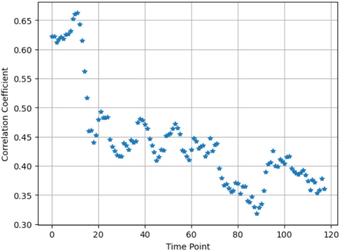
The means along with +/−2 standard errors derived from the fitted Beta distributions for the sample correlation coefficients of the voxel pairs between two thalamic ROIs (the Thalamus ROI 8 and Thalamus ROI 9) over all time points from one subject (HC subject 10,159).

FIGURE 8.

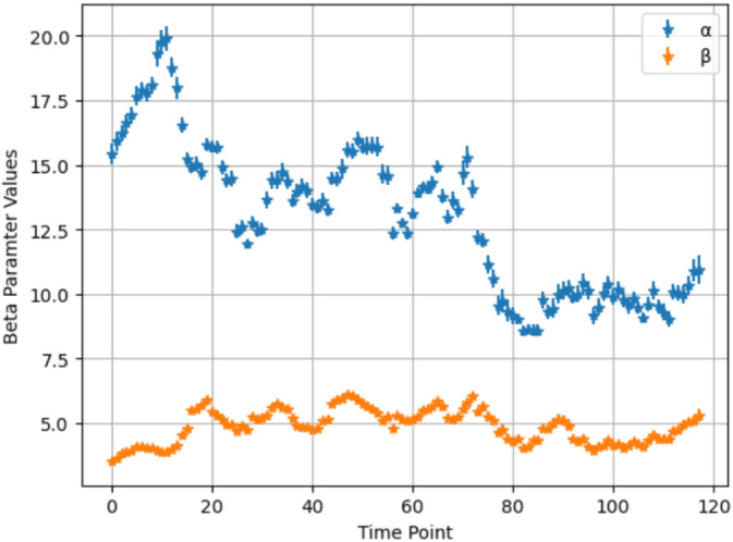
The fitted beta distribution shape parameters along with +/−2 standard errors for the sample correlation coefficients of the voxel pairs between two thalamic ROIs (the Thalamus ROI 8 and Thalamus ROI 9) over all time points from one subject (HC subject 10,159).

Following a similar approach, to study dynamics at the group level, we could aggregate the means derived from the fitted beta distributions of all subjects within a subject group to create a distribution of mean correlation coefficients for the group at specific time points. Figure 9 depicts the histograms of mean correlation coefficients between two ROIs at time points, 10, 50, and 100, across subjects from different groups.

FIGURE 9.

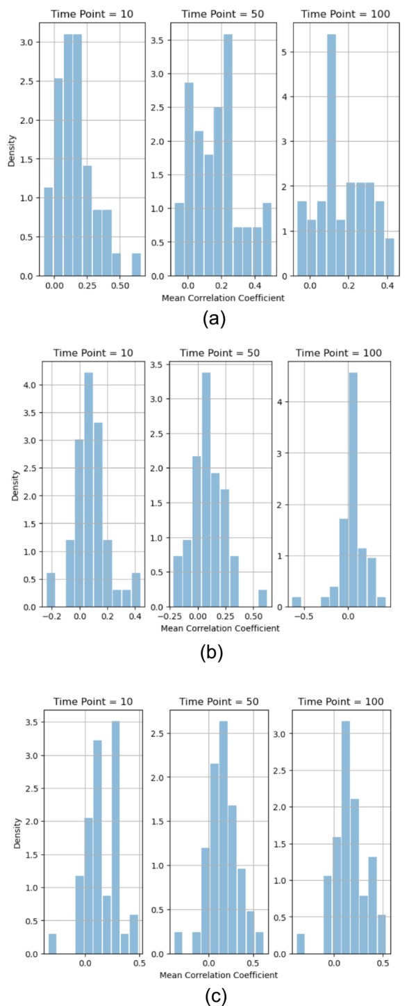
Histograms of the means derived from the fitted beta distributions for the sample correlation coefficients of the voxel pairs between two ROIs at time points, 10, 50, and 100, from different subject groups. (a) Across 48 healthy control subjects between Thalamus ROI 8 and ROI 9. (b) Across 49 schizophrenia subjects between Basal Ganglia ROI 38 and ROI 39. (c) Across 41 ADHD subjects between Cerebellum ROI 19 and ROI 20.

3.9. Distributions of Means of Correlation Coefficients Among Mental Disorders

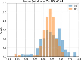
With a total of 48 HC, 41 ADHD, 48 BP, and 49 SZ subjects in our dataset, we conducted an in‐depth analysis to explore any potential variations in brain functional connectivity patterns across all ROI pairs among these distinct groups of subjects. This analysis involved capturing the dFC patterns of ROI pairs for comparison across different subject groups. Building upon our previous empirical distribution analysis, we aimed to capture the dFC patterns as empirical probability distributions. To achieve this, we decided to aggregate the dFC variations over time into a single dFC pattern for each subject group. To identify the dFC pattern, we calculated the empirical distribution of means derived from the fitted beta distributions across all time points of an ROI pair. In a more detailed explanation, the mean for each time point between an ROI pair was computed for individual subjects. These mean values were then aggregated for all time points across all subjects within a specific group, resulting in the empirical distribution that represented the dFC pattern for that ROI pair in that group. For instance, when computing the empirical distribution of means for HC subjects, we combined all the means obtained from fitted beta distributions across all time points for the entire group of 48 HC subjects for a given ROI pair. Importantly, this dFC pattern effectively captured the variations in the means over time for the entire HC group by consolidating them into an empirical distribution. This summarization of the variations in central tendencies of correlation coefficients across all time points within a subject group into an empirical distribution as a dFC pattern enhanced the effectiveness of comparing dFC patterns between HC subjects and subjects with various mental disorders. To conduct this analysis across 186 subjects, we sampled and used 257 voxel pairs from each ROI pair to capture the dFC patterns. This approach, rather than using the full set of 257 × 257 voxel pairs, made the analysis more computationally feasible. Our tests showed that while the full set provided more samples and produced a smoother representation of the underlying distribution, the reduced set still adequately captured the distribution's properties, such as the mean, meeting the needs of our analysis. Figure 10 illustrates the empirical distributions of means, specifically corresponding to the Cerebellum ROI 40 and Cerebellum ROI 44 pair between the HC and the other groups.

FIGURE 10.

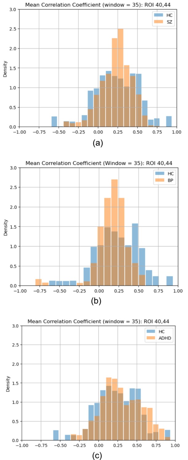
The empirical distribution of means of correlation coefficients obtained through the fitted beta distributions. (a) Cerebellum ROI 40 and Cerebellum ROI 44 pair for the HC and SZ groups. (b) Cerebellum ROI 40 and Cerebellum ROI 44 pair for the HC and BP groups. (c) Cerebellum ROI 40 and Cerebellum ROI 44 pair for the HC and ADHD groups.

3.10. Comparative Analysis of Mean Distributions

Across all the ROI pairs, we applied the two‐sample KS test to determine whether the mean distributions of the HC group differed significantly from those of the other groups: ADHD, BP, and SZ. For each group comparison (e.g., HC vs. ADHD), we performed one test per ROI pair, resulting in a total of 1176 tests. To adjust for multiple comparisons, we applied Bonferroni correction, setting the significance level at ~0.00004 (0.05 divided by 1176). We compiled and summarized the –log ₁₀ p‐values from all the ROI pairs in Table 3. A –log ₁₀ p‐value exceeding 4.4 (−log ₁₀ 0.00004) indicated a statistically significant difference in the ROI pair. It is worth noting that given the large sample sizes used in our analysis (n = number of subjects × number of sliding windows = 5664 for the HC group, n = 4838 for the ADHD group, n = 5664 for the BP group, n = 5782 for the SZ group), the KS test could be highly sensitive, detecting even subtle distinctions between samples of different groups. Out of 1176 ROI pairs considered, 175 ROI pairs (95.2%) (HC vs. ADHD), 159 ROI pairs (93.4%) (HC vs. BP), and 152 ROI pairs (92.1%) (HC vs. SZ) exhibit a –log ₁₀ p‐values larger than 4.4. This indicates significant differences in dFC patterns between the HC group and each of the other groups: ADHD, BP, and SZ, respectively, for these specific ROI pairs.

TABLE 3.

The –log ₁₀ p‐values of the two‐sample Kolmogorov–Smirnov between the HC group and other groups, ADHD, BP, and SZ, from all the ROI pairs.

	HC versus ADHD		HC versus BP		HC versus SZ
–Log 10 p	Count of ROI pairs	%	Count of ROI pairs	%	Count of ROI pairs	%
0 to 4.4	56	4.8%	78	6.6%	93	7.9%
> 4.4 to 25	651	55.4%	641	54.6%	641	54.5%
> 25 to 75	393	33.4%	409	34.8%	380	32.3%
> 75 to 275	76	6.4%	47	4%	62	5.3%
Total	1176	100%	1176	100%	1176	100%

We further calculated effect sizes for the significant ROI pairs, taking into account the sample sizes, to identify those showing the most pronounced differences. The distribution of these effect sizes is detailed in Table 4. Notably, the ADHD group had the highest proportion of ROI pairs (7.5%) showing more substantial differences (effect size > 0.0035), whereas the BP group had the lowest (2.9%).

TABLE 4.

The effect sizes for the significant ROI pairs comparing the HC group with other groups, ADHD, BP, and SZ.

	HC versus ADHD		HC versus BP		HC versus SZ
Effect size	Count of ROI pairs	%	Count of ROI pairs	%	Count of ROI pairs	%
0 to 0.001	46	4.1%	80	7.3%	106	9.8%
> 0.001 to 0.002	580	51.8%	609	55.5%	592	54.7%
> 0.002 to 0.0035	410	36.6%	377	34.3%	341	31.5%
> 0.0035 to 0.007	84	7.5%	32	2.9%	44	4.1%
Total	1120	100%	1098	100%	1083	100%

3.11. Comparative Analysis of dFC Patterns Across Brain Networks

To delve deeper into the comparative analysis of dFC patterns between the HC group and other groups, ADHD, BP, and SZ, we specifically examined ROI pairs with an effect size greater than 0.0035. These ROI pairs were further organized by brain networks, distinguishing between intra‐network connections (spanning DMN, CON, SDN, and FPN) and internetwork connections (including DMN‐CON, DMN‐SDN, DMN‐FPN, CON‐SDN, CON‐FPN, and SDN‐FPN). Additionally, the ROI pairs were categorized based on the mean values of their connectivity patterns as either hyper‐connectivity or hypoconnectivity. This classification was achieved by comparing the mean from the mean distribution of the HC group with the corresponding means from the mean distributions of the other groups. In cases where the mean of the other group, compared to the HC group, was greater, the ROI pair was characterized as demonstrating hyper‐connectivity. Conversely, if the mean was smaller, it indicated hypo‐connectivity. Table 5 summarizes the connectivity patterns between the HC group and other groups, ADHD, BP, and SZ of the ROI pairs, organized by brain networks. Both ADHD and SZ groups displayed substantial hyperconnectivity within the SDN‐FPN internetwork connections. Moreover, the SZ group showed the highest proportion of hyperconnectivity connections across all connections compared to the other two groups. Such distinctive dFC patterns linked with different mental disorders have the potential to function as biomarkers for differentiating individuals with distinct mental health conditions.

TABLE 5.

Connectivity patterns between the HC group and other groups, ADHD, BP, and SZ of the ROI pairs with an effect size greater than 0.0035, organized by brain networks.

	HC versus ADHD		HC versus BP		HC versus SZ
	Hyper‐connectivity	Hypo‐connectivity	Hyper‐connectivity	Hypo‐connectivity	Hyper‐connectivity	Hypo‐connectivity
DMN	4	0	1	1	2	0
CON	0	0	0	1	0	0
SDN	7	16	0	4	2	2
FPN	2	1	0	1	1	1
DMN‐CON	4	1	1	2	3	1
DMN‐SDN	12	6	0	1	6	0
DMN‐FPN	8	2	0	1	4	0
CON‐SDN	3	2	1	1	2	1
CON‐FPN	1	1	2	1	3	3
SDN‐FPN	11	3	9	5	10	3
TOTAL	52	32	14	18	33	11

4. Discussion

In this study, we examined the statistical characteristics of the empirical distribution of functional connectivity in voxel signals, measured with Pearson's correlation. This unique method provided us with a statistical framework for understanding the dynamic nature of functional connectivity patterns. Our study provided for the first time a strong statistical evidence about the dynamic nature of functional connectivity. It also offered an objective characterization of dFC through an examination of the empirical distributions of the correlation coefficients. Our results paved the way for an accurate statistical understanding and modeling of dFC.

A key assumption in our approach was that the signal time series from each ROI were generated from an underlying random process. Additionally, each voxel within a given ROI was considered a realization of the same underlying random process for that particular ROI. This consideration was crucial as it allowed us to treat voxel signals as representative samples of the underlying random process, enabling us to examine the essential characteristics of the random process and the dynamic nature of functional connectivity patterns. All voxels within a specific ROI were presumably engendered by the same random process, as our ROIs (4‐mm radius spheres) were assumed to be, functionally, relatively homogenous.

Similar to prior studies, we employed the widely adopted sliding‐window correlation as a metric for dFC. This method involved computing correlation coefficients between pairs of voxels from two ROIs at each time point, offering insights into the dynamic changes in functional connectivity between any two ROIs.

In this study, we investigated the distribution of correlation coefficients in voxel signals, finding that the beta distribution served as a parsimonious and highly accurate approximation. When the signals exhibit bivariate normal distribution, the exact PDF of the sample correlation coefficient is well established. Notably, in the special case where the correlation coefficient is ρ = 0, the distribution of the sample correlation coefficient follows a beta distribution. Motivated by the expectation that the distribution would remain stable when the correlation coefficient deviated from ρ = 0, we explored whether the exact PDF of the sample correlation coefficient could be effectively approximated with a beta distribution. Our expectation was validated through numerical simulation and the KLD measure (cf. Figure 4). This result allowed us to adopt the simpler, more flexible, and convenient beta distribution for modeling the distribution of correlation coefficients. This approach offered us a valuable advantage over working with the exact distribution, simplifying our analytical process, and enhancing our ability to analyze dFC patterns with greater ease and effectiveness.

One key research objective was to validate the existence of dFC, a phenomenon that had been debated and was yet to be conclusively demonstrated. Our goal here was to establish that the observed dFC was not merely a result of random fluctuations inherent in an underlying stationary random process but rather a phenomenon that displayed a significant non‐stationarity in the empirical distribution of correlation coefficients. More specifically, to establish non‐stationarity within the correlation coefficient distribution of signals derived from voxel pairs connecting two specific ROIs over time, we employed two distinct methods. First, we utilized the two‐sample Kolmogorov–Smirnov test to measure the dissimilarity of the empirical distribution of correlation coefficients between two ROIs of a HC subject across different time points and against all other time points. The result from this analysis clearly indicated statistically significant differences in the correlation coefficient distribution at different time points, affirming its non‐stationary characteristics under temporal shifts. This finding provided initial support for the proposition that the underlying correlation coefficient distribution was non‐stationary.

Second, as a complementary approach, we fitted a beta distribution to the correlation coefficients from voxel pairs between two ROIs of the HC subject at each distinct time point. The results of this modeling underscored substantial variations in the correlation coefficient distribution over time. The means along with +/−2 standard errors derived from these fitted beta distributions showcased dynamic fluctuations, ranging from 0.32 to 0.67. This dynamic alteration in the central tendencies of correlation coefficients provided further evidence of the non‐stationarity that manifests when shifted in time occur. In essence, this finding effectively ruled out the distribution as being strong‐sense stationary or weak‐sense stationary. Additionally, the fitted beta distribution shape parameters along with +/−2 standard errors also exhibited a broad spectrum of variations. Collectively, this comprehensive examination substantiated the dynamic and non‐stationary nature inherent in the correlation coefficient distribution as it evolved across different time points. These findings consistently replicated across diverse subjects, underscoring a reliable and broadly applicable pattern. Overall, this evidence strongly supported the existence of dFC.

To assess the usefulness of our approach, we further investigated any potential variations in brain dFC patterns among different mental disorders, including ADHD, BP, and SZ. For that purpose, we computed the empirical distribution of means of correlation coefficients across time. These means were derived from the fitted beta distributions, which characterized the correlation coefficients between any two ROIs across all time points. This empirical distribution was computed separately for each subject group, encompassing HC, ADHD, BP, and SZ subjects. With these distributions of means available for all possible ROI pairs within each distinct subject group, we subsequently assessed and compared the differences between the HC group and the other groups, namely ADHD, BP, and SZ. This comparative analysis enabled us to identify and quantify the differences in dFC patterns between controls and those with different mental disorders.

In our analysis of 1176 ROI pairs originating from four distinct brain networks, we identified noteworthy findings. Specifically, we focused on the ROI pairs displaying prominent differences (effect size > 0.0035), organized by brain networks. It is important to highlight that conflicting findings exist in the literature. Our comprehension of hyperconnectivity and hypoconnectivity patterns within different brain networks for various mental disorders remains inconclusive (Li et al. 2019; Unschuld et al. 2014). Nevertheless, our distinctive analysis approach, involving the comparison of the empirical distribution of means of correlation coefficients, despite focusing solely on non‐cortical regions, consistently aligned with certain findings reported in the literature. In line with existing literature (Li et al. 2019; Unschuld et al. 2014), it was evident that numerous connections within and between brain networks demonstrated patterns of both hyperconnectivity and hypoconnectivity. Examples included the intranetwork connections within the SDN in the SZ group, as well as the internetwork connections between the CON‐SDN across the ADHD, BP, and SZ groups. Patients with BP were previously reported to demonstrate hypoconnectivity in the intranetwork connections within the FPN and CON (Yoon et al. 2021). Our results supported and aligned with these findings. Previous research linked hyperconnectivity within the DMN to cognitive impairment in patients with SZ (Unschuld et al. 2014). Our study not only replicated this finding but also found significant hyperconnectivity specifically within the SDN‐FPN internetwork connections among subjects with SZ. Previous study indicated that children with ADHD often demonstrated hyperconnectivity within the DMN (Barber et al. 2014). Our findings aligned with this prior result, as we also observed hyperconnectivity within the DMN in subjects with ADHD.

Our comparative analysis across various mental disorders yielded several intriguing and noteworthy findings. The ADHD group exhibited pronounced hypoconnectivity within the SDN intranetwork connections. The BP group exhibited a distinctive pattern characterized by pronounced hypoconnectivity within SDN intranetwork connections. Remarkably, the BP group stood out as the only one to display more hypoconnectivity connections than hyperconnectivity connections among all the identified connections. In contrast, the SZ group distinguished itself by demonstrating marked hyperconnectivity, with the highest proportion of hyperconnectivity connections when compared to the other two groups. These findings collectively emphasized the intricate interplay of connectivity patterns both within and between brain networks across the studied groups. Presently, there is a notable absence of dependable and objective biomarkers for numerous mental disorders, hindering early detection and treatment efforts (Rashid et al. 2016). While the dFC patterns discerned in this study did not yet yield specific biomarkers for identifying distinct mental disorders, the mean distributions did reveal distinctive dFC patterns associated with different mental disorders.

This study had some limitations that warrant additional investigation. Our analysis was based on a single resting‐state fMRI dataset. To establish the robustness and generalizability of our findings, it is imperative to extend our research to additional resting‐state fMRI datasets with larger sample sizes, including fMRI data collected at different magnetic field strengths. While we comprehensively explored 49 subcortical and cerebellar ROIs originating from four specific brain networks, it is important to replicate this analysis on cortical regions and at variable ROI sizes. In summary, addressing these limitations through further research endeavors will advance our understanding of dynamic functional connectivity patterns in neurotypicals as well as in people with diverse neurological and mental deficits, with the ultimate aim to identify robust dFC‐based markers for both diagnosis and prognosis purposes. Now we turn to the question of the ROI selection. ROI selection can significantly impact the extracted signals for subsequent analyses in both task‐based and task‐free fMRI (e.g., Tong et al. 2016; Moghimi et al. 2022). There is no gold‐standard parcellation or ROI selection procedure in fMRI literature, and the most useful ROI selection approach depends on users' relevant questions of interest. Here, we followed the same rationale as Seitzman et al. 2020 by using spherical ROIs, to ensure relatively functionally homogenous ROIs. Although this approach is not frequently used, compared to the typical ROI selection based on functional or anatomical atlases, it does guarantee similar sizes for all ROIs to calculate the different inter‐region correlations and statistical parameters straightforwardly. Our approach also works for ROIs with different sizes, such as those predefined in existing atlases and parcellations, providing that ROIs are functionally homogenous. This is why we recommend the use of functional parcellations based on resting‐state fMRI (e.g., Fan et al. 2016; Gordon et al. 2016; Joliot et al. 2015; Schaefer et al. 2018; Seitzman et al. 2020), with the expectation that defined ROIs would include voxels that are part of the same functional network.

5. Conclusion

In conclusion, our study marked a significant milestone as the first to effectively demonstrate the non‐stationarity within the empirical probability distribution of functional connectivity, measured by the Pearson's correlation of fMRI signals (Lurie et al. 2020). Our remarkable finding was a direct result of our distinctive approach employed in this study. Diverging from the conventional method of aggregating signals from numerous voxels into a limited set of region‐based signals as a pre‐processing step, our study capitalized on individual voxel signals. This unique approach granted us access to a diverse collection of realizations stemming from the same underlying random process. This not only enabled accurate characterization of the empirical probability distribution, but also facilitated the assessment of its temporal variations and non‐stationarity.

Author Contributions

Abd‐Krim Seghouane was the originator of the research idea. Winn W. Chow conceived and designed the study, analyzed and interpreted the data, and drafted the manuscript under the supervision of Abd‐Krim Seghouane. Mohamed L. Seghier critically revised the manuscript for important intellectual content and provided contributions to the content. The authors are listed according to their relative contributions.

Conflicts of Interest

The authors declare no conflicts of interest.

Supporting information

Data S1: Supporting Information.

Data Availability Statement

The data that support the findings of this study are available in Openneuro at https://openneuro.org/, reference number ds000030. These data were derived from the following resources available in the public domain: – UCLA Consortium for Neuropsychiatric Phenomics LA5c Study, https://openneuro.org/datasets/ds000030/versions/00016.

References

- Ahrends, C. , and Vidaurre D.. 2023. “Dynamic Functional Connectivity (No. arXiv:2301.03408).” arXiv. 10.48550/arXiv.2301.03408. [DOI]
- Allen, E. A. , Damaraju E., Plis S. M., Erhardt E. B., Eichele T., and Calhoun V. D.. 2014. “Tracking Whole‐Brain Connectivity Dynamics in the Resting State.” Cerebral Cortex 24, no. 3: 663–676. 10.1093/cercor/bhs352. [DOI] [PMC free article] [PubMed] [Google Scholar]
- Anderson, T. W. 2003. An Introduction to Multivariate Statistical Analysis. John Wiley & Sons Inc. [Google Scholar]
- Barber, A. D. , Jacobson L. A., Wexler J. L., et al. 2014. “Connectivity Supporting Attention in Children With Attention Deficit Hyperactivity Disorder.” NeuroImage: Clinical 7: 68–81. 10.1016/j.nicl.2014.11.011. [DOI] [PMC free article] [PubMed] [Google Scholar]
- Bear, M. , Connors B., and Paradiso M. A.. 2020. Neuroscience: Exploring the Brain ‐ With Navigate 2 Premier Access: Enhanced 4th Edition. 4th ed. Jones & Bartlett Learning. [Google Scholar]
- Biswal, B. , Yetkin F. Z., Haughton V. M., and Hyde J. S.. 1995. “Functional Connectivity in the Motor Cortex of Resting Human Brain Using Echo‐Planar MRI.” Magnetic Resonance in Medicine 34, no. 4: 537–541. 10.1002/mrm.1910340409. [DOI] [PubMed] [Google Scholar]
- Chai, B. , Walther D. B., Beck D. M., and Fei‐Fei L.. 2009. “Exploring Functional Connectivity of the Human Brain Using Multivariate Information Analysis.” In Proceedings of the 22nd International Conference on Neural Information Processing Systems, 270–278. Curran Associates, Inc. [Google Scholar]
- Chang, C. , and Glover G. H.. 2010. “Time‐Frequency Dynamics of Resting‐State Brain Connectivity Measured With fMRI.” NeuroImage 50, no. 1: 81–98. 10.1016/j.neuroimage.2009.12.011. [DOI] [PMC free article] [PubMed] [Google Scholar]
- Chaubey, Y. P. , and Mudholkar G. S.. 1978. “A New Approximation for Fisher's Z.” Australian Journal of Statistics 20, no. 3: 250–256. 10.1111/j.1467-842X.1978.tb01107.x. [DOI] [Google Scholar]
- Damaraju, E. , Allen E. A., Belger A., et al. 2014. “Dynamic Functional Connectivity Analysis Reveals Transient States of Dysconnectivity in Schizophrenia.” NeuroImage: Clinical 5: 298–308. 10.1016/j.nicl.2014.07.003. [DOI] [PMC free article] [PubMed] [Google Scholar]
- Fan, L. , Li H., Zhuo J., et al. 2016. “The Human Brainnetome Atlas: A New Brain Atlas Based on Connectional Architecture.” Cerebral Cortex 26, no. 8: 3508–3526. 10.1093/cercor/bhw157. [DOI] [PMC free article] [PubMed] [Google Scholar]
- Fransson, P. , and Marrelec G.. 2008. “The Precuneus/Posterior Cingulate Cortex Plays a Pivotal Role in the Default Mode Network: Evidence From a Partial Correlation Network Analysis.” NeuroImage 42, no. 3: 1178–1184. 10.1016/j.neuroimage.2008.05.059. [DOI] [PubMed] [Google Scholar]
- Gordon, E. M. , Laumann T. O., Adeyemo B., Huckins J. F., Kelley W. M., and Petersen S. E.. 2016. “Generation and Evaluation of a Cortical Area Parcellation From Resting‐State Correlations.” Cerebral Cortex 26, no. 1: 288–303. 10.1093/cercor/bhu239. [DOI] [PMC free article] [PubMed] [Google Scholar]
- Gorgolewski, K. J. , Durnez J., and Poldrack R. A.. 2017. “Preprocessed Consortium for Neuropsychiatric Phenomics Dataset.” F1000Research 6: 1262. 10.12688/f1000research.11964.2. [DOI] [PMC free article] [PubMed] [Google Scholar]
- Joliot, M. , Jobard G., Naveau M., et al. 2015. “AICHA: An Atlas of Intrinsic Connectivity of Homotopic Areas.” Journal of Neuroscience Methods 254: 46–59. 10.1016/j.jneumeth.2015.07.013. [DOI] [PubMed] [Google Scholar]
- Karahanoğlu, F. I. , and Van De Ville D.. 2015. “Transient Brain Activity Disentangles fMRI Resting‐State Dynamics in Terms of Spatially and Temporally Overlapping Networks.” Nature Communications 6, no. 1: 1. 10.1038/ncomms8751. [DOI] [PMC free article] [PubMed] [Google Scholar]
- Kenney, J. F. , and Keeping E. S.. 1957. Mathematics of Statistics. 3rd ed. Toronto: D. Van Nostrand. [Google Scholar]
- Leonardi, N. , Richiardi J., Gschwind M., et al. 2013. “Principal Components of Functional Connectivity: A New Approach to Study Dynamic Brain Connectivity During Rest.” NeuroImage 83: 937–950. 10.1016/j.neuroimage.2013.07.019. [DOI] [PubMed] [Google Scholar]
- Li, S. , Hu N., Zhang W., et al. 2019. “Dysconnectivity of Multiple Brain Networks in Schizophrenia: A Meta‐Analysis of Resting‐State Functional Connectivity.” Frontiers in Psychiatry 10: 482. 10.3389/fpsyt.2019.00482. [DOI] [PMC free article] [PubMed] [Google Scholar]
- Liégeois, R. , Laumann T. O., Snyder A. Z., Zhou J., and Yeo B. T. T.. 2017. “Interpreting Temporal Fluctuations in Resting‐State Functional Connectivity MRI.” NeuroImage 163: 437–455. 10.1016/j.neuroimage.2017.09.012. [DOI] [PubMed] [Google Scholar]
- Liu, C. , Xue J., Cheng X., Zhan W., Xiong X., and Wang B.. 2019. “Tracking the Brain State Transition Process of Dynamic Function Connectivity Based on Resting State fMRI.” Computational Intelligence and Neuroscience 2019: 9027803. 10.1155/2019/9027803. [DOI] [PMC free article] [PubMed] [Google Scholar]
- Lurie, D. J. , Kessler D., Bassett D. S., et al. 2020. “Questions and Controversies in the Study of Time‐Varying Functional Connectivity in Resting fMRI.” Network Neuroscience 4, no. 1: 30–69. 10.1162/netn_a_00116. [DOI] [PMC free article] [PubMed] [Google Scholar]
- Moghimi, P. , Dang A. T., Do Q., Netoff T. I., Lim K. O., and Atluri G.. 2022. “Evaluation of Functional MRI‐Based Human Brain Parcellation: A Review.” Journal of Neurophysiology 128, no. 1: 197–217. 10.1152/jn.00411.2021. [DOI] [PMC free article] [PubMed] [Google Scholar]
- Mokhtari, F. , Akhlaghi M. I., Simpson S. L., Wu G., and Laurienti P. J.. 2019. “Sliding Window Correlation Analysis: Modulating Window Shape for Dynamic Brain Connectivity in Resting State.” NeuroImage 189: 655–666. 10.1016/j.neuroimage.2019.02.001. [DOI] [PMC free article] [PubMed] [Google Scholar]
- Poldrack, R. A. 2007. “Region of Interest Analysis for fMRI.” Social Cognitive and Affective Neuroscience 2, no. 1: 67–70. 10.1093/scan/nsm006. [DOI] [PMC free article] [PubMed] [Google Scholar]
- Power, J. D. , Cohen A. L., Nelson S. M., et al. 2011. “Functional Network Organization of the Human Brain.” Neuron 72, no. 4: 665–678. 10.1016/j.neuron.2011.09.006. [DOI] [PMC free article] [PubMed] [Google Scholar]
- Preti, M. G. , Bolton T. A., and Van De Ville D.. 2017. “The Dynamic Functional Connectome: State‐Of‐The‐Art and Perspectives.” NeuroImage 160: 41–54. 10.1016/j.neuroimage.2016.12.061. [DOI] [PubMed] [Google Scholar]
- Rashid, B. , Arbabshirani M. R., Damaraju E., et al. 2016. “Classification of Schizophrenia and Bipolar Patients Using Static and Dynamic Resting‐State fMRI Brain Connectivity.” NeuroImage 134: 645–657. 10.1016/j.neuroimage.2016.04.051. [DOI] [PMC free article] [PubMed] [Google Scholar]
- Savva, A. D. , Mitsis G. D., and Matsopoulos G. K.. 2019. “Assessment of Dynamic Functional Connectivity in Resting‐State fMRI Using the Sliding Window Technique.” Brain and Behavior: A Cognitive Neuroscience Perspective 9, no. 4: e01255. 10.1002/brb3.1255. [DOI] [PMC free article] [PubMed] [Google Scholar]
- Schaefer, A. , Kong R., Gordon E. M., et al. 2018. “Local‐Global Parcellation of the Human Cerebral Cortex From Intrinsic Functional Connectivity MRI.” Cerebral Cortex 28, no. 9: 3095–3114. 10.1093/cercor/bhx179. [DOI] [PMC free article] [PubMed] [Google Scholar]
- Seitzman, B. A. , Gratton C., Marek S., et al. 2020. “A Set of Functionally‐Defined Brain Regions With Improved Representation of the Subcortex and Cerebellum.” NeuroImage 206: 116290. 10.1016/j.neuroimage.2019.116290. [DOI] [PMC free article] [PubMed] [Google Scholar]
- Shine, J. M. , Koyejo O., Bell P. T., Gorgolewski K. J., Gilat M., and Poldrack R. A.. 2015. “Estimation of Dynamic Functional Connectivity Using Multiplication of Temporal Derivatives.” NeuroImage 122: 399–407. 10.1016/j.neuroimage.2015.07.064. [DOI] [PubMed] [Google Scholar]
- Spencer, A. P. C. , and Goodfellow M.. 2022. “Using Deep Clustering to Improve fMRI Dynamic Functional Connectivity Analysis.” NeuroImage 257: 119288. 10.1016/j.neuroimage.2022.119288. [DOI] [PMC free article] [PubMed] [Google Scholar]
- Stnava . 2023. ANTs by stnava . http://stnava.github.io/ANTs/.
- Thomas Yeo, B. T. , Krienen F. M., Sepulcre J., et al. 2011. “The Organization of the Human Cerebral Cortex Estimated by Intrinsic Functional Connectivity.” Journal of Neurophysiology 106, no. 3: 1125–1165. 10.1152/jn.00338.2011. [DOI] [PMC free article] [PubMed] [Google Scholar]
- Thompson, W. H. , and Fransson P.. 2016. “On Stabilizing the Variance of Dynamic Functional Brain Connectivity Time Series.” Brain Connectivity 6, no. 10: 735–746. 10.1089/brain.2016.0454. [DOI] [PMC free article] [PubMed] [Google Scholar]
- Tong, Y. , Chen Q., Nichols T. E., et al. 2016. “Seeking Optimal Region‐Of‐Interest (ROI) Single‐Value Summary Measures for fMRI Studies in Imaging Genetics.” PLoS One 11, no. 3: e0151391. 10.1371/journal.pone.0151391. [DOI] [PMC free article] [PubMed] [Google Scholar]
- Unschuld, P. G. , Buchholz A. S., Varvaris M., et al. 2014. “Prefrontal Brain Network Connectivity Indicates Degree of Both Schizophrenia Risk and Cognitive Dysfunction.” Schizophrenia Bulletin 40, no. 3: 653–664. 10.1093/schbul/sbt077. [DOI] [PMC free article] [PubMed] [Google Scholar]
- Wager, T. D. , and Lindquist M. A.. 2015. Principles of fMRI. Leanpub. https://leanpub.next/principlesoffmri. [Google Scholar]
- Yeo, B. T. , Krienen F. M., Chee M. W., and Buckner R. L.. 2014. “Estimates of Segregation and Overlap of Functional Connectivity Networks in the Human Cerebral Cortex.” NeuroImage 88: 212–227. 10.1016/j.neuroimage.2013.10.046. [DOI] [PMC free article] [PubMed] [Google Scholar]
- Yoon, S. , Kim T. D., Kim J., and Lyoo I. K.. 2021. “Altered Functional Activity in Bipolar Disorder: A Comprehensive Review From a Large‐Scale Network Perspective.” Brain and Behavior: A Cognitive Neuroscience Perspective 11, no. 1: e01953. 10.1002/brb3.1953. [DOI] [PMC free article] [PubMed] [Google Scholar]
Associated Data
This section collects any data citations, data availability statements, or supplementary materials included in this article.
Supplementary Materials