

Abstract
In this article, we discuss the qualitative analysis and develop an optimal control mechanism to study the dynamics of the novel coronavirus disease (2019-nCoV) transmission using an epidemiological model. With the help of a suitable mathematical model, health officials often can take positive measures to control the infection. To develop the model, we assume two disease transmission sources (humans and reservoirs) keeping in view the characteristics of novel coronavirus transmission. We formulate the model to study the temporal dynamics and determine an optimal control mechanism to minimize the infected population and control the spreading of the novel coronavirus disease propagation. In addition, to understand the significance of each model parameter, we compute the threshold quantity and perform the sensitivity analysis of the basic reproductive number. Based on the temporal dynamics of the model and sensitivity analysis of the threshold parameter, we develop a control mechanism to identify the best control policy for eradicating the disease. We then conduct numerical experiments using large-scale numerical simulations to validate the theoretical findings.
Keywords: Epidemiological model, Threshold parameter, Stability analysis, Optimal control theory, Numerical simulation
Subject terms: Computational biology and bioinformatics, Diseases, Mathematics and computing
Introduction
Many types of viruses in the coronavirus family can infect people and cause illnesses like the common cold and severe acute respiratory syndrome (SARS). Two epidemics of coronaviruses, SARS and Middle East Respiratory Syndrome Coronavirus (MERS), have been reported in the past two decades with more than 10 thousand confirmed cases and 1600 deaths1–3. Initially, the infection of Middle East Respiratory Syndrome Coronavirus (MERS) was identified in Saudi Arabia while spreading in many other countries4. In late 2019, a severe respiratory illness identified with a causative agent isolated from a single patient reported in Wuhan, China, known as the novel coronavirus (2019-nVoV)5. The scientific data clarify that animals were the virus’s primary transmission source, but most cases increase due to interaction between vulnerable and infected people. The signs of a new coronavirus infection include fever, cough, exhaustion, breathing issues, etc. The novel coronavirus was a public health emergency of international concern, according to the World Health Organization (WHO), which declared it a global pandemic due to a pressing issue.
Due to the new nature of the disease, the coronavirus has been identified as a global danger and has drawn the interest of numerous researchers. Infectious disease epidemiology has a rich literature (see for detail6–9). Various epidemiological models investigated the dynamics and control analysis of different infectious diseases10–12. Similarly, the new coronavirus has a rich literature, and numerous articles have been reported to study the future spread of the disease dynamics. Particularly, a model was introduced to investigate the new coronavirus transmission by Wu et al. in13. To estimate the outbreak based on human interaction, a computational study has been reported by Imai et al.14. Further, the infectivity of the newly reported virus has been investigated by Zhu et al.15. Likewise, various other studies have been performed to investigate the dynamics of 2019-nCoV virus transmission16–20.
The biological interpretation of the novel coronavirus reveals that the pandemic rises due to close contact of human interactions but the initial transmission source is an animal. Therefore environmental reservoirs play an essential role in the spreading of novel coronavirus transmission. Thus, we assume both transmission sources according to the characteristics of the novel infection and follow the classical susceptible-infected-recovered (SIR) model to develop a new mathematical model while studying the temporal dynamics of the novel coronavirus disease propagation. More specifically, we assume humans and reservoirs as a source of disease transmission and propose an epidemiological model by considering the extending version of the classical susceptible-infected-recovered (SIR) model. In addition, we formulate an optimal control mechanism to minimize novel coronavirus spreading in the community. We first show the model validity to discuss the mathematical and biological properties of the epidemic problem that is under consideration. We calculate the threshold parameter and show its sensitivity to estimate the role of every epidemic parameter involved in the modeling process of the proposed problem. It will clarify the importance and role of every model parameter. We also investigate the stability of the model to find the stability conditions using linear stability analysis. Further, we develop a control mechanism based on the temporal dynamics of the model and sensitivity analysis to identify the best control policy for eradicating the disease. A large-scale numerical simulation will be also performed to validate the theoretical results of the model by providing numerical experiments.
Mathematical formulation of the model
We examine the dynamics of the newly reported disease in this section by keeping in view the properties of 2019-nCoV to propose the model, whose schematic process is given in the flowchart as depicted in Fig. 1. For this purpose, the different compartments of humans and reservoirs are taken. We also take multiple transmission routes, i.e. from humans and reservoirs. We impose some assumptions on the model stated as:
All the state variables and parameters are taken to be positive or non-negative.
The total human population is classified into three different compartments and one class of reservoir.
Humans and reservoirs play a crucial role in the rise of the pandemic, so both are taken as a source of disease transmission.
All newborns will lead to the susceptible group of individuals because there is still no evidence regarding vertical transmission of the disease.
Thus, the epidemic problem can take the combination of the coupled nonlinear differential equation which looks like:
Figure 1.

The schematic diagram for the transmission of 2019-nCoV.
 |
1 |
with non-negative initial size of population
 |
2 |
where  is the proportion of newborns.
  and
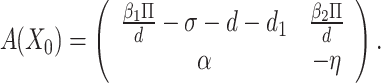
and  are the disease transmission rates occurring from humans and reservoirs, respectively. d demonstrates the natural mortality of humans while
  is the death rate of infected humans. The recovery/removal rate of infected individuals is denoted by
  . The parameter
  is the ratio at which the infected individuals contribute virus in terms of the environmental reservoirs, while
  is the removal rate of the virus.
Existence analysis and positivity
We show the mathematical and biological feasibility of the epidemic problem that is under consideration. Since the sum of the humans population is define as  , which implies that
  . Now, from the last equation of the system (1), we can re-write
 |
implies that
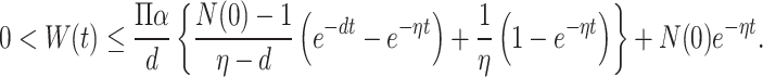 |
Clearly, W(t) is bounded; thus, all the model solutions are bounded as well as positively invariant, and the feasible region is given as
 |
3 |
In addition, let us assume that  and B represents Banach space, then
 |
4 |
We define the norm on B as 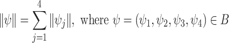 and suppose that the positive cone of
  is
is  , then from Eq.(4),
  . Thus the state space of the proposed system (1), takes the following form
 |
5 |
Let L is the linear operator and  , then
 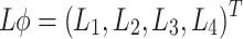 , where
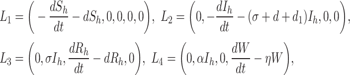 |
6 |
and D(L) is the domain, then  . In which
  is the set of absolutely continues functions on
  . Now we define the nonlinear operator M, such that
  by
by
 |
7 |
Let  , then the proposed system (1) can be written as
 |
8 |
where  . Now to prove the existence of solution of the above system (8), we follow21,22, thus we have the following results.
Theorem 2.1
For each  , there exist a maximal interval of existence
  and a unique continues mild solution
  ,
,  for Eq.(8), such that
 |
9 |
Proposition 2.1
Let us assume the initial conditions (2) of the proposed model, then the solutions of the proposed model are positive for all  .
.
Proof
Let  , then the solution of the first equation of system (1) looks like
 |
10 |
Obviously the L.H.S of Eq. (10) is positive i.e.,  . Similarly, it can be shown that the solution of the second, third, and fourth equations of the model (1) are non-negative.
Stability analysis
We investigated that the proposed epidemic problem is mathematically and biologically feasible. To discuss the temporal dynamics, we perform stability of the model with the aid of linear stability theory. We calculate the model equilibria and find the threshold quantity (basic reproductive number). We also derive the stability conditions to characterize whether the disease dies out or persists.
Threshold quantity and dynamical analysis of the model equilibria
To find the stability conditions, we study the qualitative behavior of the proposed epidemic problem. We first calculate the disease-free equilibrium and then the threshold quantity. For this, we set all the states equations of the model equating to zero except  , which gives
  is the disease-free state of the considered model, where
  .
.
In addition, the threshold quantity represents the average number of secondary infections produced by a single infective whenever introduced into a susceptible population. This will identify what happens if an infected agent enters into the population of susceptible. One of the examples of the 2019-nCoV is given by Fig. 2, which suggests that the coronavirus spreads faster than the estimation of WHO. This study was organized between Jan 2020 and Feb 2020, and the estimate ranged from 1.4-6.49 with 3.28 of average and 2.79 of a median23. In this case, the estimated threshold value is high, and it is essential to control the pandemic by reducing the weight of the reproductive number. So here, we are going to figure out the threshold quantity ( ) of the model that is under consideration following the methodology of24. We then discuss the detailed sensitivity of the threshold parameter to find the relation of all parameters to the disease propagation. This type of analysis will be beneficial to optimize the value of the threshold quantity. Based on the next-generation matrix method, we calculate matrix F, and V is given by
Figure 2.
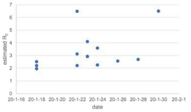
Estimated values of the threshold quantity  ) for the 2019-nCoV virus in China.
 |
11 |
The threshold quantity is the dominant eigenvalue of the matrix ( ), given by
 |
12 |
From the above Eq. (12), it is clear that the threshold quantity for the proposed problem consists of two parts, which describe that there are two different transmission routes, one from the infected individuals and the other from reservoirs to the susceptible populations.
Sensitivity analysis
To find the relation of every parameter with the threshold quantity to the disease transmission and then its severeness, we use the formula  by following25. Once we calculate the indices of the threshold quantity, we can analyze the sensitivity of each parameter to the disease transmission and its prevalence. Using the above formula, we obtain the following indices
 |
13 |
It is very much clear from the Eq. (13) that the relation between  and parameters
  is direct. But it is indirect with the parameters given by
  , which certify that if the parameters value of
  increases, the value of the threshold parameter will also increase significantly. In contrast, a decrease in the parameters value of
  causes increases in threshold quantity. Now to control the spread of coronavirus disease, we focus on optimizing the value of the parameters that have a direct relation with threshold quantity and maximizing the value of those parameters with an inverse relation. More precisely, we take some feasible values of the parameters to find the percentage of the sensitivity indices and their relative impact on the threshold quantity numerically. Let us assume the biological feasible values of the parameters, i.e.,
  ,
,  ,
,  ,
,  and
and  to find the numerical value of the sensitivity indices and their relative percentage impact on the threshold quantity. Using the above numerical values, we calculate the following indices, i.e.,
  ,
,  ,
,  ,
,  . The biological interpretation of these sensitivity indices shows that the increase or decrease in the value of
  , say, for example, 10 percent, would increase or decrease the value of
  by 9.999990210 percent as shown Fig. 4. In addition, if we increase or decrease the value of
  and
and  by 10 percent, collectively affects the value of the threshold quantity by 0.001958158 percent, see Fig. 3b. Similarly, from the sensitivity indices of
  and
and  , we observe that the influence of these parameters on the threshold quantity is negative, in which an increase leads to a decrease in threshold quantity. For example, an increase of 10 percent in the value of
  and
and  would decrease the value of the threshold quantity by 0.9870088245 and 0.0009790790415 respectively, for instance, see Fig. 3a,b.
Figure 4.
The graphical results show the sensitivity analysis of the threshold quantity ( ) and its relative impact against the variation of various epidemic parameters
  . We use the numerical values of other parameters
  ,
,  ,
,  ,
,  .
.
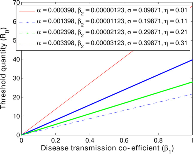
Figure 3.

The graphical results show the sensitivity analysis of the threshold quantity ( ) and its relative impact against the variations of various epidemic parameters
  . For this analysis, the numerical values of the parameters used are
 ,
,  ,
,  ,
,  ,
,  ,
,  ,
,  .
.
Dynamical analysis
To discuss the model dynamics at the disease-free state using the theory of dynamical systems, we state the following results.
Theorem 3.1
If  is less than unity, i.e.
  , then the model is stable asymptotically at
  .
.
Proof
Since the considered model reveals that  is not explicitly involved in all other equations, we assume only the three equations of the model, while investigating the dynamics of the proposed epidemic problem. Let
  is the Jacobian the model (1) at
  , then
 |
14 |
Obviously,  has an eigenvalue,
  . For the remaining, we take the following reduced matrix
 |
15 |
The local dynamics of the epidemic problem depend on the nature of the eigenvalues of the Jacobian matrix. So,  is negative while the eigenvalues of (15) will be negative if the Routh- Hurwitz criteria hold. We noted that the trace and determinant of matrix (15) are respectively negative and positive if the
  is less than unity, such that
 |
16 |
and
 |
17 |
Equations (16)–(17) implies that Routh–Hurwitz criteria satisfies under the condition that  , so we conclude that the model (1) is stable asymptotically in local sense if
  .
.
For the global dynamics around  , we define a function
  , such that
 |
18 |
In the above Eq. (18),  ,
,  are arbitrary positive constants. We differentiate
  temporally and assume the values of the positive constants, i.e.,
  ,
,  , then arrives at the following equation
 |
Obviously  is negative if
  and
and  . Moreover,
  if
if  and
and  . Therefore, the well-known LaSalle invariance principle or simply invariance principle26 implies that
  is globally asymptotically stable.
To determine the dynamics of the model at the endemic equilibrium, we assume that  be the endemic equilibrium of the proposed model, which is obtained by setting
  ,
,  ,
,  ,
,  at the steady state, then the corresponding disease endemic equilibrium leads to
  , where the following system of equation defines the components of the endemic state:
 |
19 |
It can be noted from the above Eq. (19) that the endemic state of the model exists only in the case whenever  . Thus we state the following result.
Lemma 3.2
The endemic state  , of the proposed problem (1) exists only in the case
  .
.
To discuss the model temporal dynamics around the endemic state we prove the following theorem.
Theorem 3.3
If the conditions  and
and  holds then
  is asymptotically stable.
Proof
We use the theory of linear stability analysis to discuss the dynamics of the model at  . Let
. Let  be the Jacobian matrix of the model (1) around
  , then
 |
20 |
To discuss the local dynamics, we find the characteristic polynomial of (20) as
 |
21 |
where
 |
22 |
According to linear stability analysis, the proposed model around endemic equilibrium (19) is stable if all eigenvalues of the Jacobian matrix (20) are negative. One may follow the Routh- Hurwitz criteria to discuss the properties of the Jacobian matrix (20). Roots (eigenvalues) of the above Eq. (21) are negative, if Routh-Hurwitz criteria  i.e.
i.e.  ,
,  and
and  holds. It can be noted from Eq. (22) that
  and
and  are positive under the condition that
  , while
  is calculated and given by the following expression
 |
23 |
Clearly  , whenever
  , so
, so  satisfied if
  . Thus, model (1) is asymptotically stable at
  if
if  .
.
For the global dynamics, we assume a function  by the following equation
 |
24 |
We differentiate  and making use of some simple algebra, we get
 |
It could be noted from the above equation that  if and only if
  ,
,  , and
, and  ,
,  ,
,  ,
,  . Thus we conclude that according to the invariance principle the disease endemic state
  is globally asymptotically stable, if
  and
and  .
. 
Optimal control
Keeping in mind the model dynamics and sensitivity of the threshold parameter, we analyse a control mechanism with the aid of optimal control theory. It can be noted that the maximum sensitivity index parameter in the epidemic parameters is  , whose value is 0.9999990210. This indicates that the increase of 10 percent in
  causes the increase of 9.999990210 percent in the value of
  . Therefore, the very first step to control the spread needs much attention to minimize the value of this parameter. With the help of the control variable, isolation of infected and non-infected (
 ), we can reduce and optimize the spreading in the community. Similarly, the index of
  is 0.000097079, which affects the threshold quantity by 0.00097079 percent. To minimize the value of this parameter, we use the control variable, (
 ), which physically represents personal protection, e.g., wearing of mass, washing hands, etc. The index of
  is 0.000097079, which variates the threshold quantity by 0.00097079 percent. We must reduce this by taking the
  control variable. Moreover, the collective variation of
  and
and  affect the threshold quantity by 0.9870088245 and 0.0009790790415. Here, we need to increase the values of these parameters because the increase would decrease the threshold quantity value. For this, we assume
  , a control measure representing infected individuals’ treatment. Thus we are now in a position to take the set of control variables symbolized by u(t) and define as
  , where
  is used for the isolation of infected individuals from the community, while
  represents the personal protection including wearing of masks, washing hands, etc. Similarly, the control variable
  represents the treatment of infected individuals, as it is clear that Corona has no proper treatment, so this control means that treatment which strengthens the immunity system and
  is the control variable which is used for minimizing the value of the parameter
  . Placing the control variables, we arrive at the following control problem:
 |
25 |
subject to the system, which is the extended version of Eq. (1) as defined by
 |
26 |
with
 |
27 |
In the above Eq. (25),  and
and  ,
,  ,
,  ,
,  ,
,  and
and  are the weight constants in which
  and
and  represent the relative cost of the infected population and reservoir, while
  ,
,  ,
,  and
and  measure the associated cost of
  ,
,  ,
,  and
and  , respectively. The goal of our control problem is very clear from the objective functional (25): to control the disease by maximizing the recovered and reducing the infected, and the reservoir by taking into account the cost of controls. We obtain the cost function at
  , such that
 |
28 |
subject to the control system (26), where U in the above Eq. (28) is called control set and defined by the following equation
 |
29 |
In addition, first, we prove that such controls exist. Following the methodology given in27, demonstrates the existence of a solution for the proposed control system whenever the controls are bounded, and Lebesgue’s measurable along with the initial conditions are non-negative. Re-writing the control problem as
 |
30 |
In the above system (30),  , while
  and A contain the non-linear and bounded co-efficient, and linearize matrix, respectively, such that
 |
Setting  , satisfies that
 |
where  . Also, we have
 |
where  , so L is uniformly Lipschitz continuous and
  ,
,  ,
,  and W(t) having non-negative values which implies the existence of solution to the system (26).
Thus, we describe the existence analysis with the aid of the following theorem regarding.
Theorem 4.1
Proof
Obviously, the model states and control functions have non-negative values while set U is closed and convex. In addition, the control system is bounded implying compactness. Also, the integrand in Eq.(25) is convex, therefore it investigates the existence of optimal controls. 
Optimality condition
We find the optimal solution to the control problem (25)–(26). We define the Hamiltonian and Lagrangian by assuming that if x is the state variable and u is a control function, then
 |
31 |
and
 |
32 |
where  and
and  , and
, and
 |
We now use the well-known Pontryagin Maximum Principle28 to find the optimal solution. We assume that if  is an optimal solution, then there exists a nontrivial function
  , satisfying
 |
33 |
and
 |
34 |
which is the maximality condition and  , the transversal condition holds. Using Eq. (33) to find the adjoint system and optimal value for controls with the aid of the result given below.
Theorem 4.2
We assume that  ,
,  ,
,  ,
,  are the optimal states and
  are optimal control functions for the control problem., the adjoint system looks like
 |
35 |
with terminal conditions  . Furthermore, the set of optimal control functions is defined by
  , where
 |
36 |
Proof
The adjoint variables (35) can be derived from the direct use of the Eq. (33), and the transversal conditions can be obtained from  . In addition, to find the optimal value of the controls, we set
  , and solve for
  ,
,  ,
,  and
and  .
. 
Numerical experiments
The verification of our analytical results will be analyzed with the help of some computational findings. The large-scale simulations are based on both quantitative and qualitative analysis. We take some of the parameters from the literature while some are adjusted based on the analytical results. We use purely numerical methods, i.e., Runge-Kutta method (RKM) of the 4th order to simulate the model based on numerical data along with time interval of  units. More precisely, we take the parameters value i.e.,
  ,
,  ,
,  ,
,  ,
,  ,
,  ,
,  and
and  to verify the analytical findings of the model at the disease-free state. We calculate
  and
and  for the above parameter’s value as (9.814987767, 0, 0, 0) and 0.004373289660. Thus, we perform the numerical experiments for the model (1) using the above parametric values, and obtain the results as depicted by Fig. 5, which ensures the verification of the result stated by Theorem 3.1. Perturbing the initial sizes of the compartmental population along with the parametric ratios and interval of time, the solution goes to the disease-free equilibrium irrespective of its initial sizes, which ensures that the model is stable at
  . Further, the theoretical interpretation states that in case of
  , each solution curve of the susceptible population approximately taking 300 to 400 days to reach the equilibrium value 9.814987767 as shown in Fig. 5a. Similarly, the dynamics of infected and recovered population in the case when
  describe that the solution curves of
  and
and  respectively take approximately 50 and 400 days to reach its equilibrium position as shown in Figs. 5b,c. Thus, the biological interpretation states that the elimination of the 2019-nCoV virus from the community will take more time almost 12 to 13 units if
  . So it is essential to optimize and keep the value
  less than one.
Figure 5.

The dynamics of the model in the case whenever  and
and  . For this, we use the value of the parameters:
  ,
,  ,
,  ,
,  ,
,  ,
,  ,
,  and
and  .
.
Next, we assume another set of parameters value, i.e.,  ,
,  ,
,  ,
,  ,
,  ,
,  ,
,  and
and  to study the dynamics of the considered problem at the endemic state (19). We calculate the associated threshold quantity and endemic equilibrium
  , defined as:
  and
and  . Here, if
  , we take the same initial sizes of the compartmental populations. We observed that the susceptible populations decrease or increase during the initial 100 days of the infection, however after that, there will be no effect, which guarantees the stability of the susceptible individuals as shown in Fig. 6a and therefore approaches to its equilibrium position 23.73428588. The dynamics of the infected population reveal that initially, the ratio of this population increases suddenly during the initial period of the infection, i.e., up to 50 days, while later decreases day by day and attains its endemic position, i.e., 30.31567421 as shown in the Fig. 6b. From this, it could be noted that the disease will reach its endemic position. The 30.31567421 ratio of the infected population will persist in the community if the proper control measure is not implemented. Moreover, we simulate the problem to study the recovered population and reservoir dynamics as shown in Fig. 6c,d. The dynamics of the recovered population describe that in the initial days between 0 to 450 days, the ratio of recovered individuals increases or decreases while then becoming stabilized and attaining its equilibrium position 31.27631426. To control the spread, it should be characterized to increase this ratio. Finally, the ratio of reservoir increases in the initial period of the infection, i.e., between 0 to 400 days according to the dynamics of the proposed problem, while then becoming stable and reaching to its equilibrium 1261.065047. Special attention will be required to sustain the reservoir’s position to zero to control COVID-19.
Figure 6.

The dynamics of the model compartmental population in the case whenever  and
and  . For this, we use the value of the parameters are
  ,
,  ,
,  ,
,  ,
,  ,
,  ,
,  and
and  .
.
In order to discuss the impact of control analysis, we use the well-known purely numerical method Runge-Kutta method (RKM) of order 4th. We solve the optimality system, i.e., numerically, we discretize the model (1), the proposed control problem (26), and the adjoint system (35) along with the initial conditions (2)–(4), boundary conditions  and characterization of the control problem. Moreover, the value of the parameter used for this purpose are
  ,
,  ,
,  ,
,  ,
,  ,
,  ,
,  and
and  , while the values of weight constants are assumed to be
  ,
,  ,
,  ,
,  ,
,  and
and  . More precisely, the control and without a control system will be solved by the forward RKM method of order 4th and then the adjoint system by backward RKM method of order 4th with the help of terminal conditions and the solution of system (1). The numerical experiments support the suggested control mechanism as shown in Figs. 7 and 8, while in the case if we ignore the control mechanism and don’t follow the suitable control measure in the form of precautions and treatment etc., it would significantly increase and grow up the spreading of the disease throughout the World. On the other hand, the results describe that the infection will be easily eliminated once the control mechanism imposes in the true spirit.
Figure 7.

The graphical visualization of the control problem with and without controls.
Figure 8.

The plots visualizes the dynamics of time dependent controls measures.
Cost effective optimal control analysis
We discuss the most cost-effective optimal control measure among the single and combined implementation of the control measures in order to optimally determine the spread of SARS-CoV-2 at the lowest possible cost. We use incremental cost effectiveness ratio (ICER) to explore cost-effectiveness analysis29,30. To avoid dissipation of available limited resources, ICER is calculated to compare any two competing measures for controlling the spread of disease or related problems as given by the ICER formula
 |
The total cost for each of the single implementation and combined effort of the control measures is calculated from the objective functional (25), while the infection averted is obtained by calculating the difference between infectious individuals without and with control measures. Let  for
for  and
and  respectively represent the single implementation of each control measure
  , and combined effort of the four control measures. Table 1 summarizes the ICER for each and combination of the control variables
  in an increasing order of the total infection averted.
Table 1.
ICER in the order of COVID-19 cases averted by control measures.
| Control strategy | Total infection averted | Total costs | ICER |
|---|---|---|---|
 |
 |
 |
− 0.2055 % |
 |
 |
 |
− 27.1684 % |
 |
 |
 |
− 0.7759 % |
 |
 |
 |
− 58.1766 % |
 |
 |
 |
− 0.3861 % |
Using the ICER using the above formula for each 
 and
and  shown in Table 1 are calculated, respectively,
Comparing  ’s, it is seen that
  is less than any other
  for
for  . This means that
  for
for  are more costly and less effective than
  . In other words,
  dominates
  for
for  . Thus, single implementation of management control is removed from the list. As a consequence,
  and
and  are assessed in Table 2 using similar procedure.
Table 2.
Comparison between  and
and  .
.
| Control strategy | Total infection averted | Total costs | ICER |
|---|---|---|---|
 |
 |
 |
− 0.2055 % |
 |
 |
 |
− 0.3861 % |
It is revealed in Table 2 that  is dominated by
  since
since  is greater than
  . This implies that
  is less costly and more effective than
  . Hence, single implementation of preventive measure is excluded from the list. This shows that combined effort of the four control measures is the most cost effective intervention capable of diminishing the burden of the novel coronavirus optimally in the host population.
Conclusions
In the current work, we studied the pandemic trend of the 2019-nCoV virus transmission. We developed an epidemiological model with control mechanism strategies to eradicate/control the virus. We studied the fundamental axioms of the model to show the mathematical and biological feasibility. Once the model is well-possed, we find the threshold parameter ( ) and discuss the detailed sensitivity, which clarifies the role of every epidemic parameter involved in the combination of the proposed model. It would be noted that the key parameters that strengthen the spread of the disease are
  , which is approximately 99.99 percent, affecting the threshold quantity’s value. Moreover, the stability analysis is also performed to determine the conditions for stabilizing the disease’s exponential spread. Based on stability analysis, the various perspective of the results is investigated numerically, which states that one of the necessary steps is to optimize the threshold quantity value and keep less than unity. Similarly, if the disease persists, then the long run of the model suggests that it attains its endemic equilibrium, which is very high and not valid for the community. For this, special attention is needed to apply some control strategies to keep this minimum. Once we observed all these situations, we designed a control mechanism based on sensitivity analysis and the dynamics of the problem, which describe that the 2019-nCoV virus infection will be easily eliminated once the control program is applied truly. All the theoretical works are justified with the aid of numerical experiments. This would be quite easy for the readers to study the dynamics of the problem.
In future, we will modify the proposed model by replacing the mass action law with standard incidence to study its significance on the novel corona virus disease dynamics.
Acknowledgements
Researchers Supporting Project number (RSPD2025R576), King Saud University, Riyadh, Saudi Arabia. This work is supported by the Natural Science Foundation of Xinjiang, China (2021D01C003). In addition, we would like to express sincere thanks to the honorable referees and the editor for their valuable comments and suggestions to improve the quality of the paper. Additionally, all authors would like to express their gratitude to the United Arab Emirates University, Al Ain, UAE, for providing financial support with Grant No. 12R283.
Author contributions
S.L. and T.K. wrote the original manuscript, performed the numerical experiments. Q.M.A. reviewed the technical parts of the paper and checked the mathematical results. T.K. and G.Z performed the formal analysis and mathematical results. S.L. and T.K conceptualized the model and perform the formal analysis. G.Z and Q.M.A. Supervision and formal analysis. F.A.A. and Q.M.A. validated all the mathematical results with care, data analysis, reviewed and restructured the manuscript, funding acquisition. All authors are agreed on the final draft of the submission file.
Data availability
All data generated or analysed during this study are included in this published article.
Declarations
Competing interests
The authors declare no competing interests.
Footnotes
Publisher’s note
Springer Nature remains neutral with regard to jurisdictional claims in published maps and institutional affiliations.
Contributor Information
Tahir Khan, Email: tahirmaths200014@gmail.com.
Qasem M. Al-Mdallal, Email: q.almdallal@uaeu.ac.ae
References
- 1.Azhar, E. I. et al. Evidence for camel-to-human transmission of mers coronavirus. N. Engl. J. Med.370(26), 2499–2505 (2014). [DOI] [PubMed] [Google Scholar]
- 2.Kim, Y. et al. The characteristics of middle eastern respiratory syndrome coronavirus transmission dynamics in south korea. Osong Public Health Res. Perspect.7(1), 49–55 (2016). [DOI] [PMC free article] [PubMed] [Google Scholar]
- 3.Al-Tawfiq, J. A. et al. Middle east respiratory syndrome coronavirus: a case-control study of hospitalized patients. Clin. Infect. Dis.59(2), 160–165 (2014). [DOI] [PMC free article] [PubMed] [Google Scholar]
- 4.Chen, Z. et al. From sars-cov to wuhan 2019-ncov outbreak: Similarity of early epidemic and prediction of future trends. CELL-HOST-MICROBE-D-20-00063, (2020).
- 5.Backer, J. A., Klinkenberg, D. & Wallinga, J. Incubation period of 2019 novel coronavirus (2019-ncov) infections among travellers from wuhan, china, 20–28 january 2020. Eurosurveillance25(5) (2020). [DOI] [PMC free article] [PubMed]
- 6.Wang, Y. & Cao, J. Global dynamics of a network epidemic model for waterborne diseases spread. Appl. Math. Comput.237, 474–488 (2014). [Google Scholar]
- 7.Khan, T., Zaman, G. & Chohan, M. I. The transmission dynamic and optimal control of acute and chronic hepatitis b. J. Biol. Dyn.11(1), 172–189 (2017). [DOI] [PubMed] [Google Scholar]
- 8.Ali, N., Zaman, G. & Chohan, M. I. Global stability of a delayed hiv-1 model with saturations response. Appl. Math.11(1), 189–194 (2017). [Google Scholar]
- 9.Farayola, M. F., Shafie, S., Siam, F. M. & Khan, I. Mathematical modeling of radiotherapy cancer treatment using caputo fractional derivative. Comput. Methods Programs Biomed.188, 105306 (2020). [DOI] [PubMed] [Google Scholar]
- 10.Vives-Gilabert, Y. et al. Classification model based on strain measurements to identify patients with arrhythmogenic cardiomyopathy with left ventricular involvement. Comput. Methods Programs Biomed.188, 105296 (2020). [DOI] [PubMed] [Google Scholar]
- 11.Zaman, G., Kang, Y. H. & Jung, I. H. Stability analysis and optimal vaccination of an sir epidemic model. Biosystems93(3), 240–249 (2008). [DOI] [PubMed] [Google Scholar]
- 12.Abboubakar, H., Kamgang, J. C. & Tieudjo, D. Backward bifurcation and control in transmission dynamics of arboviral diseases. Math. Biosci.278, 100–129 (2016). [DOI] [PubMed] [Google Scholar]
- 13.Wu, J. T., Leung, K. & Leung, G. M. Nowcasting and forecasting the potential domestic and international spread of the 2019-ncov outbreak originating in wuhan, china: a modelling study. The Lancet395(10225), 689–697 (2020). [DOI] [PMC free article] [PubMed] [Google Scholar]
- 14.Imai, N., Cori, A., Dorigatti, I., Baguelin, M., Donnelly, C. A., Riley, S. & Ferguson, N. M. Report 3: transmissibility of 2019-ncov. In Imperial College London, (2020).
- 15.Zhu, H., Guo, Q., Li, M., Wang, C., Fang, Z., Wang, P., Tan, J., Wu, S. & Xiao, Y. Host and infectivity prediction of wuhan 2019 novel coronavirus using deep learning algorithm. bioRxiv (2020).
- 16.Rothe, C. et al. Transmission of 2019-ncov infection from an asymptomatic contact in Germany. N. Engl. J. Med. (2020). [DOI] [PMC free article] [PubMed]
- 17.Read, J. M., Bridgen, J. R., Cummings, D. A., Ho, A. & Jewell, C. P. Novel coronavirus 2019-ncov: Early estimation of epidemiological parameters and epidemic predictions. MedRxiv (2020). [DOI] [PMC free article] [PubMed]
- 18.Abboubakar, H. & Racke, R. Mathematical modeling of the coronavirus (covid-19) transmission dynamics using classical and fractional derivatives (2022).
- 19.Zheng, Q. et al. Treating sars-cov-2 omicron variant infection by molnupiravir for pandemic mitigation and living with the virus: a mathematical modeling study. Sci. Rep.13(1), 5474 (2023). [DOI] [PMC free article] [PubMed] [Google Scholar]
- 20.Kubra, K. T., Ali, R., Alqahtani, R. T., Gulshan, S. & Iqbal, Z. Analysis and comparative study of a deterministic mathematical model of sars-cov-2 with fractal-fractional operators: a case study. Sci. Rep.14(1), 6431 (2024). [DOI] [PMC free article] [PubMed] [Google Scholar]
- 21.Webb, G. Population models structured by age, size, and spatial position. In Structured population models in biology and epidemiology, pp. 1–49, Springer (2008).
- 22.Inaba, H. Mathematical analysis of an age-structured sir epidemic model with vertical transmission. Disc. Contin. Dyn. Syst. B6(1), 69 (2006). [Google Scholar]
- 23.Hellewell, J. et al. Feasibility of controlling covid-19 outbreaks by isolation of cases and contacts. Lancet Global Health (2020). [DOI] [PMC free article] [PubMed]
- 24.Earn, D., Brauer, F., van den Driessche, P., & Wu, J. Mathematical epidemiology (2008).
- 25.Khan, T., Ullah, Z., Ali, N. & Zaman, G. Modeling and control of the hepatitis b virus spreading using an epidemic model. Chaos Solitons Fractals124, 1–9 (2019). [Google Scholar]
- 26.LaSalle, J. P. The stability of dynamical systems Vol. 25 (Siam, 1976). [Google Scholar]
- 27.Kamien, M. & Schwartz, N. Dynamic optimization, vol. 31 of advanced textbooks in economics. North-Holl, Amsterdam, The Netherlands (1991).
- 28.Aseev, S. M. & Kryazhimskii, A. The pontryagin maximum principle and optimal economic growth problems. Proc. Steklov Inst. Math.257(1), 1–255 (2007). [Google Scholar]
- 29.Asamoah, J. K. K. et al. Global stability and cost-effectiveness analysis of covid-19 considering the impact of the environment: using data from ghana. Chaos Solitons Fract.140, 110103 (2020). [DOI] [PMC free article] [PubMed] [Google Scholar]
- 30.Akanni, J., Akinpelu, F., Olaniyi, S., Oladipo, A. & Ogunsola, A. Modelling financial crime population dynamics: Optimal control and cost-effectiveness analysis. Int. J. Dyn. Control8, 531–544 (2020). [Google Scholar]
Associated Data
This section collects any data citations, data availability statements, or supplementary materials included in this article.
Data Availability Statement
All data generated or analysed during this study are included in this published article.