Numerical Fresnel models of Fresnel zone plates for plane wave at angle of incidence

Abstract

Diffractive optical elements (DOEs) are increasingly used in electro-optical systems due to their design flexibility, which offers advantages over refractive optics. Although determining the point spread function (PSF) is straightforward when the plane wave is parallel to the surface normal of DOE, a comprehensive method is needed for the plane waves with an angle of incidence. Therefore, this paper proposes a general approach in order to determine the PSF under non-normal illumination of plane waves. Although the numerical PSF is specifically proposed for the Fresnel zone plate (FZP) diffractive lens, the method is adaptable to any DOE. The simulation results were validated against the Zemax optical design software for angular incidences ranging from − 60° to + 60⁰, and the results were shared. Additionally, the paraxial approximation of the PSF was proposed and verified using ZEMAX for angular incidences between −10° and + 10°. Finally, a simplified approximation for the Fresnel number, applicable to FZPs was proposed. Consequently, this research presents a novel method that can be applied to all types of DOEs for determining the numerical PSF non-normal illumination of plane waves. The proposed approach also allows for the calculation of the modulation transfer function (MTF) for diffractive optical elements in such scenarios. By incorporating the angle of incidence into PSF analysis, this work makes a significant advancement in the field of diffractive optics.

Introduction

Diffractive optical elements (DOEs) are increasingly being recognized as a promising alternative to conventional refractive optics in electro-optical systems. A key factor behind this shift is the ability of DOEs to correct optical aberrations. By meticulously designing the surface profiles of the diffractive optics, optical aberrations can be compensated, which typically would require multiple lenses or complex optical assemblies. This capability streamlines the optical design process, minimizes the number of components needed, and can enhance overall image quality. Furthermore, DOEs allow for the integration of complex optical functions into a single element. While traditional refractive optics often necessitate multiple lenses and components to perform tasks such as beam shaping, splitting, or wavefront control, DOEs can achieve these functions within a single element through careful surface design. This not only simplifies the optical system but also results in more compact and lightweight solutions^1–6.

DOEs are increasingly being utilized in various applications due to their numerous advantages, and their use is expected to expand in the future. Therefore, developing comprehensive DOE models will not only enhance our understanding of these elements but also enable the detailed analysis of DOEs for applications. Peng et al.⁴ focused on lightweight diffractive-refractive optics, while Grulois et al.⁵ investigated infrared cameras integrating diffractive optics, utilizing Zemax to model Fresnel lenses. Banerji et al.⁶ investigated multi-level diffractive lenses for near-infrared cameras, employing scalar diffraction theory with the Fresnel approximation. Zhang et al.^7,8 studied the Fresnel zone plate (FZP) and multiphase FZPs. Zhang et al.⁹ researched hybrid-level FZP. Whang et al.¹⁰ worked on variable focus lenses withFZPs, presenting an analytical equation for diffracted intensity at the image plane, and Li et al.¹¹ developed a zoom multifocal FZPlens. Peng et al.¹² worked on diffractive achromats for full-spectrum computational imaging, defining the PSF in terms of pupil function with phase retardation. Hu et al.¹³ concentrated on PSF modeling DOEs for diffraction efficiency. Britton et al.¹⁴ analyzed multi-focal diffractive lenses, using the Rayleigh-Sommerfeld PSF for modeling. Meem et al.^15–17 investigated flat diffractive lenses. Hallada et al.¹⁸ studied FZPs with analytical intensity distribution, while Jeon et al.²⁴ examined diffracted rotation in hyperspectral imaging, providing a closed-form PSF definition. Unal et al.^19–25 worked on combined and hybrid DOEs. Dun et al.^26,27 conducted research on achromatic diffractive optics, and Geints et al.^28,29 explored binary FZPs. Liu et al.³⁰ analyzed on axial intensity distribution of FZPs. Tsukamoto et al.³¹ investigated FZPs with variable focusing properties, and Zhou et al.³² studied the focusing properties of FZPs. Xu et al.³³ worked on the electrically controllable FZPs, and Baek et al.³⁴ worked on the learned diffractive optics. Jeong et al.³⁵ focused on the FZP utilizing sensor design.

The literature review reveals that PSFs for plane waves under angular incidence conditions have either been determined using commercial software or remain unexplored in prior studies. The generation of PSFs for advanced optical structures, such as multi-focus, multi-wavelength, or combined configurations, under angular incidence plane waves typically requires the creation of custom optical surfaces or DLL files within commercial software^36–42. This process introduces significant complexity and limits accessibility.

To address this gap, there is a significant need for analytical or numerical methods capable of accurately simulating PSFs for FZPs under angular incidence of plane waves. This study aims to develop a PSF determination method that explicitly incorporates angular incidence conditions, thereby overcoming this deficiency in the existing literature. The proposed method in this study enables the determination of PSFs for any complex optical structure.s

Theoretical background

The Huygens-Fresnel principle is a foundational method for analyzing both near-field and far-field diffraction effects. This principle suggests that every point on a wavefront behaves as a source of spherical secondary wavelets. These wavelets, emanating from various points, interact and interfere with one another. The overall wavefront is formed by the combined effect of these secondary wavelets.

In essence, the Huygens-Fresnel principle proposes that a wavefront can be viewed as a combination of spherical wavelets originating from distinct points on the wavefront. As the wavefront moves through space, its shape and behavior are determined by how these wavelets interfere and combine with each other. This concept applies to explaining diffraction phenomena in both near and far-field scenarios. When the distance between the image plane and lens plane is large, the exponential terms in the Huygens-Fresnel integral can be expanded using the Binomial Expansion method. As a result, the Huygens-Fresnel integral can be rewritten in the following modified form^43,44.

1

The amplitude distribution at the object plane is represented by , while denotes the amplitude distribution at the image plane in the equation. is the wavelength and is the distance between the lens and the image plane. The coordinates and represents horizontal and vertical positions in the lens plane, while and correspond to the horizontal and vertical coordinates in the image plane. These coordinates define the spatial mapping between the lens plane and the image plane. The Huygens-Fresnel integral describes the propagation from the lens plane to the image plane, as shown in Fig. 1. When the object plane is sufficiently far from the lens plane, the incoming light can be approximated as arriving from infinity. In this scenario, assuming geometric optical propagation, there is no phase difference between the light rays arriving at different points on the lens plane grid. This allows the use of one-step propagation instead of the more complex two-step propagation. However, a phase change still occurs between the light interacting with the back and the front surface of the lens plane, due to the optical properties of the diffractive lens. By incorporating these considerations and reformulating the equation in terms of the Fourier transform, the field distribution is modified by the aperture function of the lens. Consequently, the Huygens-Fresnel integral can be redefined using the Fourier transform () and the aperture function () of the lens. Under these assumptions, the amplitude distribution in the image plane can be defined as follows in terms of the Fourier transform between spatial frequency and spatial domains^43,44,46.

2

Fig. 1.

Two-step plane wave and angle of incidence plane wave propagation. The blue line indicates the angle of the incident plane wave beam propagation direction, and the black line shows the parallel beam propagation direction. The beam propagates from the object plane to the image plane while passing the lens plane. is the angle of incidence in the horizontal direction and is the angle of incidence in the vertical direction.

The Point Spread Function (PSF) is a fundamental concept in optical systems. It describes how an optical system responds to a point source of light, showing the light intensity distribution in the image plane. In real-life scenarios, most of the imaging systems were defined in terms of the incoherent PSF. For incoherent illumination, the PSF is calculated as the absolute square of the coherent point spread function. The mathematical definition of the incoherent PSF (), as detailed in references²⁵, is expressed as follows.

3

FZPs can be broadly categorized into two main types based on how their zones affect the focus. The distinction between these two types lies in their unique methods of altering the phase at the focal point. The first type is the amplitude-type FZP, where, each zone transmits or blocks the light. At the focal point, the transmitted zones produce a phase of π. The second main type is the phase FZP, in which each zone introduces a phase shift of 2π at the focal point. Figure 2b illustrates the structural layout of an amplitude-type FZP, showing its opaque and transmissive regions. The white regions represent the transmissive zones, while the black regions correspond to the opaque zones. Each transmissive region contributes to the focal point with a π phase in the first diffraction order⁴⁵.

Fig. 2.

FZP parameters. (a) is focal length and Fresnel zone relation and (b) is Fresnel zones and substrate schematic. t₀ is the substrate thickness and t₁ is the opaque material thickness.

The FZP was chosen for its simplicity, making it an ideal choice for validating the proposed PSF analysis in the context of varying angles of incidence. The relationship between the first-order focal and the Fresnel zone’s radius has been defined in the following equation.

4

In this context, is the mth zone radius and corresponds to the Fresnel zone number. The equation defining this relation was derived by neglecting the higher-order terms in the triangulation relation depicted in Fig. 2a. The higher-order terms can be neglected because their contributions are negligible compared to the dominant terms in the equation. The focal length of FZP and its diameter () relations are defined in terms of outermost zone width by the Eqs. 5 and 6 ref.^21,45. These relations provide essential parameters for analyzing and designing FZPs in terms of outermost zonewidth (). Here, M represents the total number of zones in the FZP.

5

6

The Fresnel number () is a measure used to assess the suitability of the Fresnel approximation in optical simulations⁴⁴. It is defined by adjusting the aperture size in proportion to the distance between the image plane and the lens plane, as well as the wavelength (Eq. 7). However, for FZP, the expression can be simplified when considering the focal length (Eq. 5) and the diameter (Eq. 6) of the FZP. In the case where the distance d is equal to the focal length, the Fresnel number equation can be further simplified, as defined in Eq. 8. This simplified expression in Eq. 7 proposed as an alternative for FZPs, results in a value that equals the total number of Fresnel zones (M). This provides a straightforward criterion for decision-making when compared with the Fresnel number in Eq. 7. Using only the number of Fresnel zones, one can directly determine whether to use Fresnel propagation.

7

8

The Fresnel approximation is generally considered valid when the Fresnel number is approximately equal to one. However, it can still be applied in cases where the Fresnel number slightly exceeds this value²⁵.

The aperture function for FZP diffractive optics is expressed by Eq. 9 ref.²⁷. However, this formulation assumes that the incident wavefront is a plane wave propagating parallel to the optical axis. In scenarios where the wavefront arrives at an angle of incidence, the aperture function must be redefined to account for angular effects. This redefinition ensures accurate modeling of the optical behavior under non-parallel illumination conditions, allowing for a comprehensive analysis of FZP performance in realistic optical systems.

9

, and represent the radii of the first, mth, and (m-1)th Fresnel zones, respectively, and defined as circular function and expressed as follows^25,44.

10

Point spread function model with angle of incidence

The PSF analysis is straightforward when the incident plane wave is parallel to the optical axis, as shown by the black line in Fig. 3. However, when the plane wave arrives at an angle of incidence, as shown by the blue line in Fig. 3, the PSF equation requires redefinition to accurately account for the angular effects.

Fig. 3.

Detailed representation of the projection and relative path difference.

In the case of the angle of incidence, two key physical phenomena influence the PSF. The first one is the projection effect, where the effective size of the diffractive lens changes according to the angle of incidence of the plane wave in the x’ and y’ directions. The variation is determined by the cosine of the angle of incidence, as shown in Fig. 3. Due to this reason, the effective size of the lens must be adjusted to reflect these angular changes accurately. To address this, the aperture function has been redefined to incorporate the projection effect, and the proposed formulation is presented below.

11

where is the aperture function with projection contribution. The angles of incidence in the horizontal and vertical directions are denoted as and , respectively. The second physical phenomenon associated with an incident plane wave at an angle is relative path difference. The relative path difference at each grid point changes the phase contributions, as shown in Fig. 3. The variation in path difference directly impacts the phase of the light wave at each grid point,thereby influencing the aperture function of the diffractive lens. The proposed phase contribution to the aperture function is as follows.

12

The phase matrix,, represents the phase contributions across the aperture. The terms, and denote the grid spacing in horizontal and vertical directions, respectively, while k and n represent the total grid size in horizontal and vertical directions. In the aperture function, both the projection effect and path difference phenomenon must be accounted for to accurately model the impact of non-normal plane wave illumination. This combined contribution will change the behavior of the aperture function according to the angle of incidence. The effect of non-normal plane wave illumination is incorporated by proposing a total aperture function that integrates both projection and path difference effects. The contribution of the path difference is incorporated into the aperture function through element-wise multiplication. The mathematical formulation of the proposed aperture function according to the angle of incidence is as follows.

13

The aperture function, , incorporates both the projection and path difference contributions. The two physical phenomena-projection effect and path difference-are illustrated in Fig. 3. In order to accurately model the behavior of diffractive optics under angled plane wave illumination, the aperture function was redefined to incorporate these angle of incidence effects. The projection contribution alters the amplitude distribution, while the path difference modifies the phase contributions across the aperture. Together, these factors significantly influence the overall behavior of the aperture function, demonstrating a holistic approach for accurate modeling.

Before conducting the simulations, it is essential to verify the theoretical consistency of the aperture function expression under varying angles of incidence. Specifically, the tilted aperture function () must converge to the normal aperture function () when the incidence angles are zero degrees ( and ). At zero incidence angles, in , the and terms become 0 in Eq. 12. As a result, the path difference matrix becomes an all-one matrix, and it no longer contributes to the aperture function. Furthermore, the relevant and terms are simplified to 1 in the functions. As a result, the tilted aperture function becomes identical to the normal aperture function when the incidence angles are zero.

14

If either and approaches to 90⁰, the corresponding cosine terms or in reduces to 0. Consequently functions become infinity, violating the condition less than or equal to 1. Under these conditions, the alternate criterion specified in Eq. 10 is satisfied, causing the aperture function to become zero. These behaviors align with the theoretical expectation of the aperture function for an incident wave at an angle. Consequently, the two aperture functions (normal and angle of incidence) converge to the same value. This convergence verifies the applicability of the proposed aperture function.

15

Under the paraxial approximation, the PSF must be redefined by reformulating the cosine and sine terms in the aperture function using the small-angle approximation. In this regime, where the angles involved are small, can be approximated as , and can be approximated as 1. This simplification leads to notable modifications in the aperture function’s components. Specifically, the projection term remains invariant with respect to angular variations, as it is unaffected by these approximations. In contrast, the phase term becomes explicitly dependent directly on , reflecting the influence of angular variations within the paraxial framework.

The mathematical expressions for the projection and phase terms under the paraxial approximation are detailed in Eqs. 16, 17, respectively. By combining these terms through an element-wise product, the projected aperture function for the paraxial approximation is derived. This redefined aperture function is particularly advantageous for the analysis of diffractive optics, where the small-angle assumption is valid.

16

17

Zemax and numerical simulations

The simulations within this study were conducted in two steps. Prior to the simulations, the FZP parameters were determined based on the Fresnel number. The Fresnel number is calculated by the number of Fresnel zones which is a derived parameter in this study and proposed for the FZP structures. This parameter serves as a crucial indicator for assessing whether the simulations are consistent with the Fresnel approximation. In this study, the wavelength (λ) was set to 1 µm, the focal length (f) was specified as 50 mm, and the aperture radius (r) was selected as approximately 2.4 mm, consistent with the Fresnel number 30. The parameters of the FZP are summarized in Table 1.

Table 1.

FZP parameters used in the numerical and Zemax simulations.

Parameters	Value
Focal length ()	50 mm
Propagation distance ()	50 mm
Wavelength ()	1 µm
Diameter ()	~ 2.4 mm
Total number of fresnel zones ()	30
Fresnel number ()	30

In the initial set of simulations, FZP models were developed using both Zemax and numerical methods. The resulting data are summarized in Table 2, emphasizing the incidence angles along the y-axis. Due to the circular symmetry of the FZP, angular variations along the x-axis are inherently identical to those along the y-axis. This symmetry simplifies the analysis, allowing simulations to be conducted exclusively for the y-axis without any loss of generality. The angular simulations were specifically designed to evaluate the validity of the proposed PSF under varying angular conditions.

Table 2.

Zemax and Numerical models of FZPs under tilted plane wave illumination. In the Zemax models, 3D visual representations were provided to illustrate how rays intersect with the FZP under varying angular conditions, with each angle value represented by rays in distinct colors. In the numerical FZP models, the components of the aperture functions were depicted. These components were depicted to illustrate the corresponding variations induced by changes in the angle of incidence. The scaling of the projection component ranges from 0 to 1, while the scaling of the phase component spans from − 180⁰ to 180⁰.

In both of the models, the incidence angles were systematically varied from − 60° to + 60°, encompassing a wide range of oblique and normal incidence scenarios. For clarity in the table, rays corresponding to each incidence angle in Zemax models were shown with distinct colors. The rays are visually represented based on geometric optics principles, providing a straightforward depiction of ray trajectories through the optical system. However, the actual analysis of the PSFs is conducted using physical optics propagation.

In addition, the table also presents the components of the aperture function from the numerical models, including both the phase and projected terms. The projected component of the aperture function was normalized and scaled between 0 and 1, providing a clear depiction of intensity variations across the aperture. In contrast, the phase component was scaled between –π and π, equivalent to –180° and 180°. For visualization, grayscale mapping was employed to represent these scaled values. White regions correspond to maximum values, such as peak intensity or phase, while black regions indicate minimum values, signifying areas of minimal intensity or the opposite phase extreme.

In the numerical simulations, a one-step propagation method was adopted instead of a two-step propagation⁴⁶. This approach was chosen to simplify the calculations while still providing accurate results for the given FZP parameters and maintaining consistency with the Zemax simulations. To achieve uniformity across simulation results, key parameters such as grid size, spatial resolutions of the lens plane, and the image plane were aligned between the Zemax and numerical models. In the numerical method, when performing sampling in both the spatial and spatial frequency domains, the Nyquist sampling criterion was taken into account. The simulation results are presented in Table 3, showing outcomes from both Zemax and numerical methods. The scaling used for the 2D PSF is also provided in the table. The focal point in the image plane shifts based on the angular incidence of the incoming light. Specifically, the focus moves above or below the horizontal axis (on ± y axis), depending on whether the incidence angle is positive or negative. For positive incidence angles, the focal point shifts along the -y axis of the image plane, while for negative angles, it moves along the + y axis. To facilitate meaningful interpretation and comparison of the results, the regions corresponding to the maximum intensity points are represented as 2D PSFs in the table.

Table 3.

The resulting 2D PSF distributions from the Zemax and numerical models are presented in the “2D PSF simulations” main column, with the scaling of the models displayed in the “Scaling” columns. The PSF was normalized and scaled between 0 and 1.

To analyze the PSF results in greater detail and facilitate comparison, all the PSFs are plotted along both the horizontal and vertical axes as shown in Fig. 4. The corresponding graphs are presented in Table 4. For consistency and ease of interpretation, the intensity values have been normalized to 1, ensuring a uniform scale across all plots as a dimensionless normalized value. Comparisons for the corresponding graphs obtained from ZEMAX and numerical methods are provided in Table 5.

Fig. 4.

1D PSF generation axis. (a) is the Cross X which is the horizontal axis and (b) is the Cross Y which is the vertical axis.

Table 4.

The table summarizes the 1D PSF distributions of the FZP derived from both the ZEMAX and numerical models. The FZP features a focal length of 50 mm, a diameter of approximately 2.4 mm, and is designed at 1 µm wavelength. The distributions are depicted along the horizontal and vertical axes, as depicted in Fig. 4.

Table 5.

The table provides a comparison of the one-dimensional (1D) PSF distributions of the FZP, with the distributions depicted along the horizontal and vertical axes. Cross X and Cross Y axes are illustrated in Fig. 4.

Moving on to the second set of simulations, a procedure similar to that employed in the first set was followed to ensure consistency in the methodology. The focus of these simulations was on the paraxial PSF of the FZP, which provides insights into small-angle approximation. The results of these simulations are summarized in Table 6, offering a detailed comparison and analysis of the paraxial PSF characteristics of FZP. As demonstrated by the results, there is good agreement between the Zemax simulation and the numerical simulation results. This consistency validates the general PSF proposed for FZPs, which takes into account the angle of incidence situations.

Table 6.

2D PSF simulations and their 1D comparisons of Zemax simulations and numerical PSF models under paraxial approximation. The PSFs were normalized and scaled between 0 and 1.

Discussion

Two sets of simulations were conducted to evaluate the proposed PSFs of FZPs under varying angular conditions. In the first, numerical and Zemax models were generated. In the numerical models, the aperture function was derived by incorporating both phase and projection effects, as summarized in Table 2. At a 0⁰ angle of incidence, the phase component of the aperture function becomes zero across all regions. This behavior is due to the sinθ term in the phase equation (Eq. 12), which is zero at 0⁰. Consequently, the phase component of the aperture is all 1 matrix. To validate the proposed PSF method, Zemax and numerical PSFs were plotted together, as shown in Table 5. The comparison demonstrates that the proposed PSF approach is correctly formulated, with simulation results closely matching those from Zemax. Minor discrepancies observed in some simulations are attributed to differences in resolution of both environments. Zemax dynamically adjusts its resolution for each plane during physical optics propagation, whereas the numerical method maintains a fixed resolution across all stages. To ensure compatibility, the initial and final resolutions were aligned in both simulation environments. While the numerical method involves a single propagation step, Zemax uses at least two propagation steps. However, these differences have a negligible impact on the overall results.

In the second set of simulations, the proposed paraxial PSF was generated and compared with Zemax, as detailed in Table 6. The results show that the proposed method aligns with Zemax at small angles of incidence. However, at ± 7.5⁰, minor distortions began to appear, and the deviation became more apparent at a ± 10⁰ angle of incidence. This behavior is consistent with the expectations of the small-angle approximation, where the accuracy of the paraxial PSF diminishes as the angle increases. Therefore, the simulation results confirm the paraxial approximation and validate the overall consistency of the proposed method.

As a result of the simulations and discussion, this study introduces the PSF determination method that accounts for variations in the angle of incidence addressing the limitations of traditional methods that consider only waves parallel to the optical axis for FZPs. Such conventional approaches are insufficient for conducting a comprehensive analysis of FZPs. For instance, in an imaging system using an optic with the simulated FZP with a field of view of approximately ± 15 degrees, the image quality will deteriorate toward the edge of the field of view compared to 0⁰ field. This generalized approach allows for a more accurate representation of real-world DOEs, where incident light often arrives at various angles. By incorporating the angle of incidence into the PSF analysis, the method provides a more comprehensive understanding of an DOE’s behaviour across its entire field of view.

The PSF method proposed in this study is specifically designed to account for the angular incidence of incoming plane waves for FZPs. Moreover, using this PSF, the modulation transfer function (MTF) for angular arrivals can also be derived in a straightforward manner. The proposed MTF equation for angle of incidence analysis is given below²⁵.

18

19

The approach developed in this study is versatile and applicable to both amplitude-type and phase-type diffractive optics. While the current derivation focuses on amplitude-type DOEs, the aperture function can be adapted for phase-type DOEs by incorporating the same projection and path difference effects. This extension enables a more comprehensive analysis of various types of DOEs under varying incidence angles. In addition to the points previously discussed, the Fresnel number determination approach, derived using diffractive optic parameters, offers a simplified method for determining the appropriate optical wave simulation techniques. Based solely on the zone number, it becomes possible to evaluate the compatibility of Fresnel propagation or the need for alternative propagation methods. This is one of the significant conclusions of the research. The Fresnel number approach, derived from diffractive optic parameters, provides a straightforward method for choosing appropriate simulation techniques.

The proposed PSF method was validated for various angles of incidence. However, a symmetric FZP structure was taken into account as an example. In order to test that the numerical PSF method gives correct results when defined with the appropriate aperture function in an unsymmetrical lens assembly approach, an off-axis FZP example was taken. An off-axis FZP is derived as a segment of a larger FZP structure by shifting the lens assembly along the or axes based on a predefined shift parameter and removing a portion of the structure. This process generates a new lens structure, referred to as the off-axis FZP.

The results for the off-axis FZP utilized in the secondary validation are presented in Tables 8, 9. The aperture function, accounting for the projection effect in this configuration, is defined by Eq. 20, while the path difference contribution remains consistent with Eq. 12. The parameters of the off-axis FZP used to validate the PSF in an asymmetrical configuration are detailed in Table 7.

Table 8.

Zemax and Numerical models of off-axis FZP under tilted plane wave illumination with the parameters defined in Table 7. In the Zemax models, 3D visual representations were provided to illustrate how rays intersect with the FZP under varying angular conditions, with each angle value represented by rays in distinct colors. In the numerical FZP models, the phase and magnitude components of the aperture were depicted. These components were depicted to illustrate the corresponding variations induced by changes in the angle of incidence. The scaling of the projection component ranges from 0 to 1, while the scaling of the phase component spans from − 180⁰ to 180⁰.

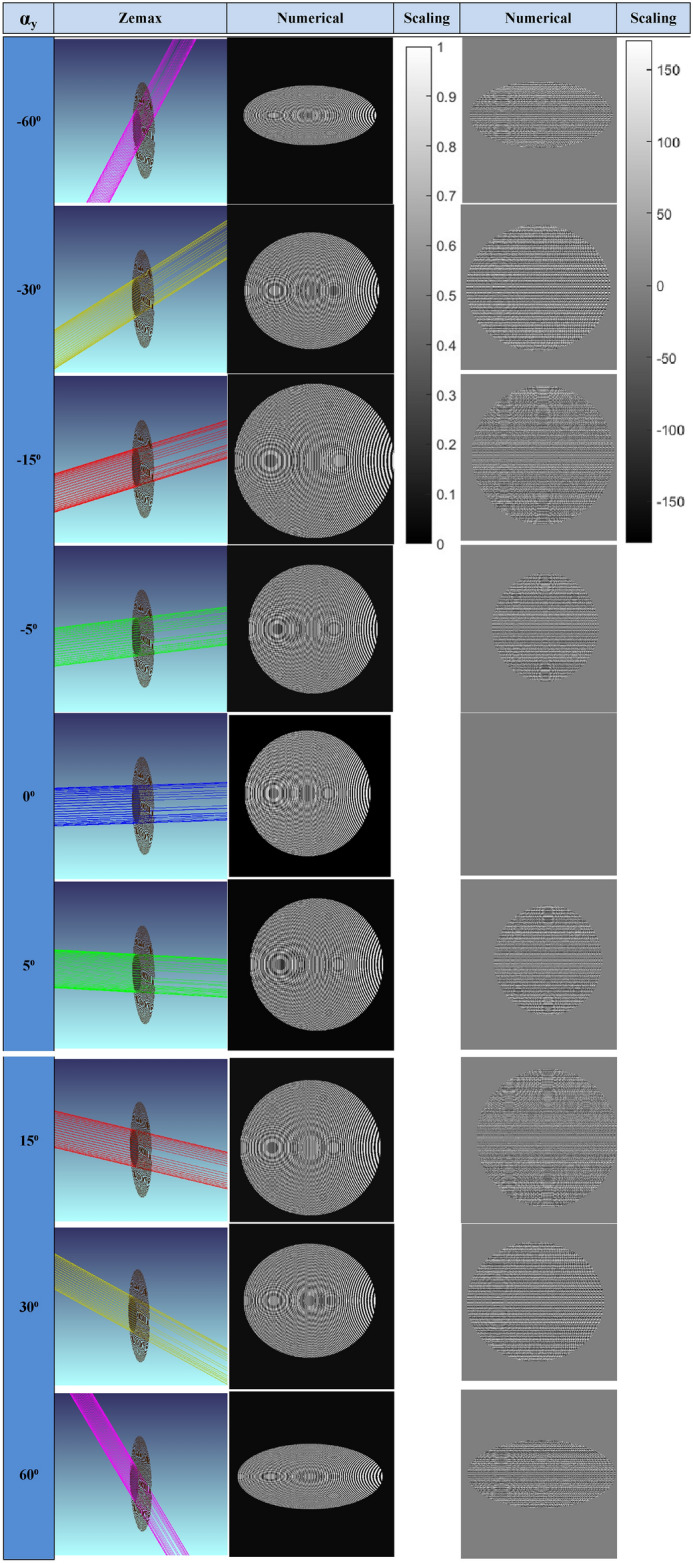
Table 9.

2D PSF simulations and their 1D comparisons of Zemax and numerical off-axis FZP models.

Table 7.

Off-axis FZP parameters used in the numerical and Zemax simulations.

Parameters	Value
Focal length ()	50 mm
Propagation distance ()	50 mm
Wavelength ()	1 µm
Shift	2 mm
Diameter ()	~ 2.4 mm
Total number of fresnel zones ()	208
Fresnel number ()	30

As detailed in Tables 8, 9, along with their corresponding Zemax models, the simulation results confirm that the proposed numerical PSF method accurately computes the PSFs for the off-axis FZP. These findings validate the effectiveness of the PSF generation method for FZP structures.

20

The PSF methods proposed in this study are specifically developed for amplitude-type FZP diffractive lenses. A similar approach can be developed for phase-type diffractive optical elements. The radii of the Fresnel zones for phase-type diffractive optical elements are defined in Eq. 21 ref.^25,31. This relation is similar to amplitude types, but it incorporates a factor of 2, which arises due to the phase shift of 2π. Using this relation, the focal length (Eq. 22) and diameter (Eq. 23) for phase-type diffractive optical elements can be derived, as outlined in Eqs. 22 and 23, respectively.

Furthermore, the Fresnel number for phase-type diffractive elements is derived in Eq. 24. Similar to amplitude type elements, the Fresnel number is simplified for phase-type diffractive optical elements to allow for easier application in practical analysis. Similarly, the aperture function of phase-type diffractive optical elements can defined in terms of projection and path difference under angular incidence conditions. The projection contribution to the aperture function is described in Eq. 25 ref.²⁵, while the path difference is the same as in FZP. As a result, the same approaches have been applied to phase-type DOEs.

21

22

23

24

25

Here is the total phase level, and the Fresnel subzone number. The parameters , , and correspond to the radii of the 1st, lth, and (l + 1)th Fresnel subzone, respectively. M represents the total number of Fresnel zones for phase-type diffractive optical elements.

In conclusion, a generalized PSF approach that takes into account variations in the angle of incidence has been investigated and verified within the scope of this study. Additionally, a simplified Fresnel number definition has been introduced for diffractive optical elements.

This work is expected to make significant contributions to the research in the field of DOEs. The proposed method specifically addresses scenarios where light is incident at various angles, extending beyond traditional analysis limited to parallel plane wave incidence to the optical axis. By providing a more accurate representation of real-world optical scenarios, this approach has the potential to enhance the design and analysis of DOEs.

Conclusion

This paper introduces a general approach for determining the PSF when plane waves are incident at an angle to the surface normal. Although the numerical PSF is specifically proposed for Fresnel zone plate (FZP) lenses, the method can be applied to any diffractive optical element (DOE) by appropriately modifying the aperture function. The simulation results were verified using the optical design software Zemax, and the findings are presented. Besides these, a simpler expression of the Fresnel number for amplitude and phase type DOEs has been proposed in order to determine the optical wave propagation method.

This research presents a novel technique applicable to all DOE types for calculating the numerical PSF under angle of incidence conditions, following aperture function modifications specific to the type of DOE. Additionally, The proposed method facilitates the computation of the modulation transfer function (MTF) for diffractive optical elements in such scenarios. By incorporating the angle of incidence into PSF analysis, this study makes a significant contribution to advancing the field of diffractive optics.

Author contributions

A. Ünal wrote the main manuscript text and figures.

Data availability

The datasets used and/or analysed during the current study available from the corresponding author on reasonable request.

Declarations

Competing interests

The authors declare no competing interests.

References

- 1.Niu, H. J. & Zhang, J. Optical system design for wide-angle airborne mapping camera with diffractive optical element. Proc. SPIE 9449 Int. Conf. Photon. Opt. Eng. (icPOE 2014)10.1117/12.2085042 (2015). [Google Scholar]
- 2.Wang, P., Mohammad, N. & Menon, R. Chromatic-aberration-corrected diffractive lenses for ultra-broadband focusing. Sci. Rep.6, 21545. 10.1038/srep21545 (2016). [DOI] [PMC free article] [PubMed] [Google Scholar]
- 3.Peng, Y., Fu, Q., Amata, H., Su, S. & Heide, F. Computational imaging using lightweight diffractive-refractive optics. Opt. Express10.1364/OE.23.031393 (2015). [DOI] [PubMed] [Google Scholar]
- 4.Peng, Y. et al. Computational imaging using lightweight diffractive-refractive optics. Opt. Express10.1364/Oe.23.031393 (2015). [DOI] [PubMed] [Google Scholar]
- 5.Grulois, T. et al. Extra-thin infrared camera for low-cost surveillance applications. Opt. Lett.10.1364/OL.39.003169 (2014). [DOI] [PubMed] [Google Scholar]
- 6.Banerji, S., Meem, M., Majumder, A. & Guevara, F. V. Ultra-thin Near Infrared camera enabled by a flat multi-level diffractive lens. Opt. Soc. Am.10.1364/OL.99.099999 (2019). [DOI] [PubMed] [Google Scholar]
- 7.Zhang, Y., Chen, J. & Yea, X. Multilevel phase Fresnel zone plate lens as a near-field optical element. Elsevier Opt. Commun.269, 271–273. 10.1016/j.optcom.2006.08.006 (2007). [Google Scholar]
- 8.Zhang, Y. J., Zheng, C.-W. & Xiao, H.-C. Improving the resolution of a solid immersion lens optical system using a multiphase Fresnel zone plate. Elsevier Opt. Laser Technol.37, 444–448. 10.1016/j.optlastec.2004.07.011 (2005). [Google Scholar]
- 9.Zhang, Z. et al. Hybrid-level fresnel zone plate for diffraction efficiency enhancement. Opt. Express10.1364/OE.25.033676 (2017).29519115 [Google Scholar]
- 10.Wang, Q., Zhang, D. W., Chen, J. B. & Zhuang, S. L. Liquid crystal variable focus lens based on Fresnel zone plate. Proc. SPIE 7279 Photon. Optoelectron. Meet. (POEM) 2008 Optoelectron. Devices Integr.10.1117/12.823827 (2009). [Google Scholar]
- 11.Li, L., Kuang, F. L., Wang, J. H., Zhou, Y. & Wan, Q. H. Zoom liquid lens employing a multifocal fresnel zone plate. Opt. Express10.1364/OE.415483 (2021). [DOI] [PubMed] [Google Scholar]
- 12.Peng, Y., Fu, Q., Heide, F. & Heidrich, W. The diffractive achromat: full spectrum computational imaging with diffractive optics. ACM Trans. Graph.10.1145/2897824.2925941 (2016). [Google Scholar]
- 13.Hu, Y., Cui, Q., Zhao, L. & Piao, M. PSF model for diffractive optical elements with improved imaging performance in dual-waveband infrared systems. Opt. Express10.1364/OE.26.026845 (2018). [DOI] [PubMed] [Google Scholar]
- 14.Britton, W. A., Chen, Y., Sgrignuoli, F. & Negro, L. D. Compact dual-band multi-focal diffractive lenses. Laser Photon. Rev.10.1002/lpor.202000207 (2021). [Google Scholar]
- 15.Meema, M. et al. Broadband lightweight flat lenses for long-wave infrared imaging. PNAS10.1073/pnas.1908447116 (2019). [DOI] [PMC free article] [PubMed] [Google Scholar]
- 16.Meem, M., Majumder, A. & Menon, R. Free-form broadband flat lenses for visible imaging. OSA Contin.10.1364/OSAC.418378 (2021). [Google Scholar]
- 17.Meem, M. et al. Imaging from the Visible to the Longwave Infrared wavelengths via an inverse-designed flat lens. Optik Express10.1364/OE.423764 (2021). [DOI] [PubMed] [Google Scholar]
- 18.Hallada, F. D., Franz, A. L. & Hawks, M. R. Fresnel zone plate light field spectral imaging simulation. Proc. SPIE 10198 Algorithms Technol. Multispectral Hyperspectral Ultraspectral Imag.10.1117/12.2261846 (2017). [Google Scholar]
- 19.Jeon, D. S. et al. Compact snapshot hyperspectral imaging with diffracted rotation. ACM Trans. Graph.38(4), 1–13. 10.1145/3306346.3322946 (2019). [Google Scholar]
- 20.Ünal, A. Semi-active laser seeker design with combined diffractive optical element (CDOE). J. Opt. India52(3), 956–968 (2023). [Google Scholar]
- 21.Ünal, A. Laser seeker design with multi-focal diffractive lens. Eng. Res. Express5, 045014. 10.1088/2631-8695/ad0024 (2023). [Google Scholar]
- 22.Ünal, A. Dual mode, imaging infrared and semi-active laser, seeker design with squinted combined diffractive optical element. J. Opt. (India)10.1007/s12596-024-01657-9 (2024). [Google Scholar]
- 23.Ünal, A. Electro-optical system, imaging infrared and laser range finder, design with dual squinted combined lens for aerial targets. J. Opt. (India)10.1007/s12596-024-02057-9 (2024). [Google Scholar]
- 24.Ünal, A. Frequency selective diffractive optical element (FSDOE). Proc. SPIE 12518 Window Dome Technol. Mater.10.1117/12.2657048 (2023). [Google Scholar]
- 25.Ünal, A. Analytical and numerical fresnel models of phase diffractive optical elements for imaging applications. Opt. Quantum Electron.10.1007/s11082-024-06906-6 (2024). [Google Scholar]
- 26.Dun, X., Wang, Z. & Peng, Y. Joint-designed achromatic diffractive optics for full-spectrum computational imaging. Proc. SPIE 11187 Optoelectron. Imaging Multimed. Technol.10.1117/12.2536617 (2019). [Google Scholar]
- 27.Dun, X. et al. Learned rotationally symmetric diffractive achromat for full-spectrum computational imaging. Optica7, 913–922. 10.1364/OPTICA.394413 (2020). [Google Scholar]
- 28.Geints, Y. E. et al. Light focusing by a binary fresnel zone plate with various design features. Atmos. Ocean. Opt.34, 714–721. 10.1134/S1024856021060099 (2021). [Google Scholar]
- 29.Yury E. Geints, Ekaterina K. Panina, and Anna V. Afonasenko. Light focusing by Fresnel phase plates with an inclined zone profile. Proc. SPIE 12341, 28th International Symposium on Atmospheric and Ocean Optics: Atmospheric Physics, 1234104, 10.1117/12.2643368. (2022)
- 30.Qi Liu, T., Liu, S., Yang, G., Li, S. . Li. & He, T. Axial intensity distribution of a micro-Fresnel zone plate at an arbitrary numerical aperture. Opt. Express29, 12093–12109 (2021). [DOI] [PubMed] [Google Scholar]
- 31.Tsukamoto, Y. & Ozaki, M. Liquid crystal micro-Fresnel zone plate with fine variable focusing properties. Opt. Contin.2, 1889–1900 (2023). [Google Scholar]
- 32.Zhou, F. et al. Optimization of the focusing characteristics of Fresnel zone plates fabricated with a femtosecond laser. J. Mod. Opt.68(2), 100–107. 10.1080/09500340.2021.1879300 (2021). [Google Scholar]
- 33.Xu, M. et al. Electrically controllable liquid crystal paraxial Fresnel zone plate based on concentric zones patterned electrode. Opt. Laser Technol.10.1016/j.optlastec.2023.109348 (2023). [Google Scholar]
- 34.S. H. Baek, H. Ikoma, D. S. Jeon, Y. Li, W. Heidrich, G. Wetzstein, M. H. Kim, Single-shot hyperspectral-depth imaging with learned diffractive optics, 10.1109/ICCV48922.2021.00265. (2021).
- 35.Baek, S. H. et al. Single-shot hyperspectral-depth imaging with learned diffractive optics. Sensors10.1109/ICCV48922.2021.00265 (2021).35009626 [Google Scholar]
- 36.Nemes-Czopf, A., Bercsényi, D. & Erdei, G. Simulation of relief type diffractive lenses in ZEMAX using parametric modelling and scalar diffraction. Appl. Opt.58(32), 8931–8942 (2019). [DOI] [PubMed] [Google Scholar]
- 37.Wood, Andy & Babington, James. Diffractive Lens Design, Theory, Design, Methodologies and Applications (IOP Publishing Ltd, 2023). [Google Scholar]
- 38.Tehrani, M. K. & Fard, S. S. M. Design of diffraction limited head mounted display optical system based on high efficiency diffractive elements. Curr. Opt. Photon.1, 150–156 (2017). [Google Scholar]
- 39.Ximin Cheng, Weimin Xie, Yu Bai, Xin Jia, and Tingwen Xing. Athermal design for infrared refractive, diffractive, reflective hybrid optical system, Proc. SPIE 9280, 7th International Symposium on Advanced Optical Manufacturing and Testing Technologies: Large Mirrors and Telescopes, 928018 10.1117/12.2068585. (2014).
- 40.He, Chuanwang, Huang, Peng, Dong, Xiaochun & Fan, Bin. Optical design of compact unobscured ground-based diffractive telescope. Optik10.1016/j.ijleo.2019.163696 (2020). [Google Scholar]
- 41.Khatri, Neha, Sonam Berwal, K., Manjunath, Bharpoor Singh, Mishra, Vinod & Goel, Saurav. Research on development of aspheric diffractive optical element for mid-infrared imaging. Infrared Phys. Technol.10.1016/j.infrared.2023.104582 (2023). [Google Scholar]
- 42.Greĭsukh, G. I., Ezhov, E. G. & Stepanov, S. A. Taking diffractive efficiency into account in the design of refractive/diffractive optical systems. J. Opt. Technol.83, 163–167 (2016). [Google Scholar]
- 43.Blahut, R. E. Theory of Remote Image Formation (Cambridge University Press, 2004). [Google Scholar]
- 44.Goodman, J. W. Introduction to Fourier Optics 2nd edn. (McGraw-Hill Series, 2005). [Google Scholar]
- 45.Atwood, D. Soft X-Rays and Extreme Ultraviolet (Cambridge University Press, 2000). [Google Scholar]
- 46.Schmidt, J. D. Numerical Simulation of Optical Wave Propagation With examples in MATLAB (SPIE Press, 2010). [Google Scholar]
Associated Data
This section collects any data citations, data availability statements, or supplementary materials included in this article.
Data Availability Statement