

Abstract
The phase portraits of the planar linear differential systems are very well known. This is not the case for the phase portraits of the planar continuous piecewise linear differential systems. In this paper we classify the phase portraits of the class of planar continuous piecewise linear differential systems of the form
in the Poincaré disc when , and prove the existence and uniqueness of limit cycles. Note that on the straight line these differential systems are only continuous.
Keywords: Continuous piecewise linear differential system, Phase portrait, Limit cycle, Poincaré disc
Introduction and Statement of the Main Result
Andronov et al. [1] started to study the piecewise linear differential systems in the 1920s for modelizing some mechanical systems, but the interest on this kind of differential systems persists up to nowadays. During the past twenty years many authors studied the dynamics of the piecewise linear differential systems, which can model many problems of mechanics, electronics, economy more accurately, see for instance [3, 4, 14, 18].
While the phase portraits of the linear differential systems
are very well known, the phase portraits of the most easiest class of continuous piecewise linear differential systems
| 1 |
with separated by the straight line are unknown. As usual the dot denotes derivative with respect to the independent variable of the differential systems, here called the time t. Note that these piecewise linear differential systems are analytic in and only continuous on the straight line . Of course the domain of definition of the continuous piecewise linear differential systems (1) is the whole plane .
The objective of this paper is to classify all topologically distinct phase portraits of the differential systems (1) in the Poincaré disc.
Recall that the phase portrait of a differential system is the description of the domain of definition of the differential system as union of all their orbits, in this way we know where the orbits born and die (i.e., their -limits and -limits), and where equilibrium points, periodic orbits and homoclinic orbits are, ..., of course if these kinds of orbits exist. In other words the phase portrait of a differential system provides all the qualitative information about the dynamics of a differential system. There are some new results about planar continuous piecewise linear differential systems with two pieces separated by a straight line, such as [9, 10], and some references therein.
A phase portrait in the Poincaré disc has the advantage with respect to a phase portrait in the plane that it controls the orbits which come from or escape to the infinity. Roughly speaking the Poincaré disc is the closed disc of radius one centered at the origin of coordinates whose interior has been identified with and its boundary, the circle , with the infinity of . For more details in the Poincaré disc see “Poincaré Compactification” section.
A periodic orbit isolated in the set of all periodic orbits of systems (1) is called a limit cycle.
Our main result is the following one.
Theorem 1
The phase portrait in the Poincaré disc of a continuous piecewise linear differential system (1) is topologically equivalent to one of the XIX phase portraits described in Fig. 1. Moreover, there exists a limit cycle in Figs. 21 and 25.
Fig. 1.

The phase portrait in the Poincaré disc of a continuous piecewise differential system (1) is topologically equivalent to one of the XIX phase portraits
Fig. 21.
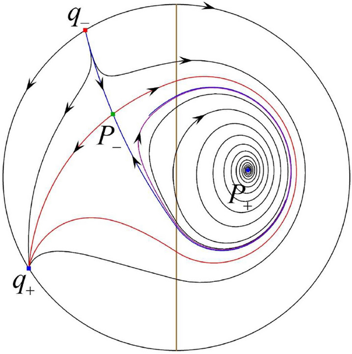
Fig. 25.
Preliminaries
The Normal Forms of the Differential Systems (1)
The continuous piecewise linear differential systems (1) depend on six parameters, but we will see that only two parameters are essential.
Since b and cannot be zero simultaneously, first we can assume that . Inspired in Proposition 3.1 of [7] we do the diffeomorphism defined by , which transforms systems (1) into the continuous piecewise linear differential systems
| 2 |
| 3 |
where , , and .
If , then doing the rescaling systems (2) and (3) become
| 4 |
| 5 |
where , , now the dot denotes derivative with respect to the new time , the upper sign takes place when , and the lower sign takes place when . Note that by exchanging the position of and systems (4) with upper sign are the same that systems (5) with lower sign, while systems (4) with lower sign are the same that systems (5) with upper sign.
Now we further do the rescaling if and systems (2) and (3) become
| 6 |
| 7 |
where , , and now the dot denotes derivative with respect to the new time . Moreover, if then the signs in (6) and (7) are negative, otherwise they are positive. When , using the rescaling , we change systems (2) and (3) to the following
| 8 |
| 9 |
Similarly, if then the signs in (8) and (9) are positive, otherwise they are negative. By , the negative situation is similar to the positive situation by exchanging the position of and .
Assuming that , we similarly do the diffeomorphism defined as , which transforms systems (1) into the continuous piecewise linear differential systems
| 10 |
| 11 |
If , then doing the rescaling systems (10) and (11) become
| 12 |
| 13 |
where , , now the dot denotes derivative with respect to the new time , the upper sign takes place when , and the lower sign takes place when . Note that , otherwise . On the other hand systems (12) with the lower sign are the same that systems (13) with the upper sign if we regard as . While systems (12) with the upper sign are also the same that systems (13) with the lower sign.
If , doing the rescaling systems (10) and (11) become
| 14 |
| 15 |
where , and now the dot denotes derivative with respect to the new time . Note that the signs of a and c determine the signs in front of x and 1 respectively. More precisely, the upper signs takes place when and respectively, and the lower signs takes place when and respectively. For convenience we denote systems (14) by and systems (15) by according to the order of signs in front of x and 1. By systems and (respectively and ) are changed to systems and (respectively and ). Thus we can obtain the 6 normal forms with only two parameters of the continuous piecewise differential systems (1) shown in Table 1, where we use and as two new parameters for convenience. This completes the proof of Table 1.
Table 1.
The 6 normal forms with only two parameters of the continuous piecewise differential systems (1)
| , if | |||
| (I): | |||
| , if | |||
| , if | |||
| (II): | |||
| , if | |||
| (III): | |||
| (IV): | |||
| (V): | |||
| (VI): | |||
In summary to classify the phase portraits of the continuous piecewise differential systems (1) is equivalent to classify the phase portraits of the continuous piecewise linear differential systems of Table 1. Note that the continuous piecewise linear differential systems of Table 1 only depend on two parameters.
Poincaré Compactification
In the proof of Theorem 1 we will use the Poincaré compactification of a planar polynomial vector field of degree d. The Poincaré compactification of , denoted by , is an induced vector field on the sphere . We call the Poincaré sphere. For more details on the Poincaré compactification see [5, Chapter 5]. Here we just introduce what we need.
Denote by be the tangent space to at the point p. Assume that is defined in the plane . Consider the central projection . This map defines two copies of , one in the open northern hemisphere and the other in the open southern hemisphere . Denote by the vector field defined on except on its equator . Clearly is identified with the infinity of . In order to extend to a vector field on (including ) it is necessary that satisfies suitable conditions. In the case that is a planar polynomial vector field of degree d, then is the only analytic extension to . On there are two symmetric copies of , one in and the other in , and knowing the behaviour of around , we know the behaviour of at infinity. The Poincaré compactification has the property that is invariant under the flow of . The equilibrium points of are called the finite equilibrium points of or of , while the equilibrium points of contained in , i.e. at infinity, are called the infinite equilibrium points of or of . It is known that the infinity equilibrium points appear in pairs diametrically opposed.
To study the vector field we use six local charts on given by , for . The corresponding local maps and are defined as for and . We denote by the value of or for any k, then (u, v) will play different roles depending on the local chart we are considering. The points of the infinity in any chart have their coordinates . The expression for in local chart is
in the local chart is
and in the local chart is .
We note that the expression of the vector field in the local chart is equal to the expression in the local chart multiplied by for .
The orthogonal projection under of the closed northern hemisphere of onto the plane is a closed disc of radius one centered at the origin of coordinates called the Poincaré disc. Since a copy of the vector field on the plane is in the open northern hemisphere of , the interior of the Poincaré disc is identified with and the boundary of , the equator of , is identified with the infinity of . Consequently the phase portrait of the vector field extended to the infinity corresponds to the projection of the phase portrait of the vector field in the Poincaré disc .
By definition the infinite equilibrium points of the polynomial vector field are the equilibrium points of contained in the boundary of the Poincaré disc, i.e. in , and the finite equilibrium points of are the equilibrium points of contained in the interior of the Poincaré disc, which of course coincide with the equilibrium points of in .
Note that for studying the infinite equilibrium points of the continuous piecewise differential systems (1) in we only need to study the infinite equilibrium points which are in the local chart and to determine if the origin of the local chart is or not an equilibrium point. While for studying the infinite equilibrium points of the continuous piecewise differential systems (1) in we only need to study the infinite equilibrium points which are in the local chart and to determine if the origin of the local chart is or not an equilibrium point.
Topological Equivalence of Two Polynomial Vector Fields
Let and be two polynomial vector fields on . We say that they are topologically equivalent if there exists a homeomorphism on the Poincaré disc which preserves the infinity and sends the orbits of to orbits of , preserving or reversing the orientation of all the orbits.
A separatrix of the Poincaré compactification is one of following orbits: all the orbits at the infinity , the finite equilibrium points, periodic orbits which are isolated in the set of periodic orbits at least by one side, when a periodic orbit is isolated in the set of periodic orbits by both sides it is a limit cycle, and the two orbits at the boundary of a hyperbolic sector at a finite or an infinite equilibrium point, see for more details on the separatrices [15, 16].
The set of all separatrices of , which we denote by , is a closed set (see [16]).
A canonical region of is an open connected component of . The union of the set with an orbit of each canonical region form the separatrix configuration of and is denoted by . We denote the number of separatrices of a phase portrait in the Poincaré disc by S, and its number of canonical regions by R.
Two separatrix configurations and are topologically equivalent if there is a homeomorphism such that .
According to the following theorem which was proved by Markus [15], Neumann [16] and Peixoto [17], it is sufficient to investigate the separatrix configuration of a polynomial differential system, for determining its global phase portrait.
Theorem 2
Two Poincaré compactified polynomial vector fields and with finitely many separatrices are topologically equivalent if and only if their separatrix configurations and are topologically equivalent.
Limit Cycles
In 1991–1992 Lum and Chua in [12, 13] conjectured that a continuous piecewise linear differential system in the plane with two pieces separated by one straight line has at most one limit cycle. We note that even in this apparent simple case, only after a difficult analysis it was possible to prove the existence of at most one limit cycle, thus in 1998 this conjecture was proved by Freire, Ponce, Rodrigo and Torres in [6]. Recently, a new easier proof that at most one limit cycle exists for the continuous piecewise linear differential systems with two pieces separated by one straight line has been done by Llibre et al. in [11]. For other results on the limit cycles of continuous and discontinuous piecewise differential systems see [2].
Proof of Theorem 1
The continuous piecewise differential systems (1) with are topologically equivalent to some of the six continuous piecewise differential systems of Table 1.
If the x-coordinate of an equilibrium point is positive (respectively negative), this equilibrium point is real (respectively virtual) for the differential systems . If the x-coordinate of an equilibrium point is negative (respectively positive), this equilibrium point is real (respectively virtual) for the differential systems . Of course if the x-coordinate of an equilibrium point is zero, then this equilibrium point is real for both differential systems and .
Limit Cycles
For continuous piecewise linear differential systems (1), we study the existence and uniqueness of their limit cycles, see “Limit Cycles” section. Note that a region enclosed by a periodic orbit of systems (1) must contain equilibrium points and the sum of the indices of the equilibrium points in a region enclosed by any periodic orbit of systems (1) is one, as it is shown in the properties 2 and 3 of [19, p. 148].
Lemma 3
For continuous piecewise linear differential systems there exists a unique limit cycle lying in the strip if either and , or and . Moreover, if and there is a continuum of periodic orbits surrounding the equilibrium point of systems bounded by a homoclinic orbit connecting the saddle of systems . And there is no periodic orbits for continuous piecewise linear differential systems
Proof
First we see that systems (respectively ) have the equilibrium point (respectively ). Furthermore, the eigenvalues of the Jacobian matrix evaluated at are . The equilibrium point is a saddle whose index is , implying that there is no periodic orbits surrounding for systems (I) in the plane .
The eigenvalues of the equilibrium point are . So if (respectively ) then (respectively ) implying that is a stable (respectively an unstable) node. If (respectively ) then are a pair of imaginary eigenvalues with negative (respectively positive) real part, implying that is a stable (respectively an unstable) focus. If then are a pair of purely imaginary eigenvalues, implying that is a center. Thus the index of the equilibrium point is one.
On the other hand we see that the divergence of systems (respectively ) is (respectively ). It implies by the Bendixson’s theorem [5, Theorem 7.10] that systems (I) have no periodic orbits surrounding when .
When by the Bendixson’s theorem systems have no periodic orbits in the half plane if . Namely systems (I) have no periodic orbits in the half plane if .
When and by the Bendixson’s theorem systems have no periodic orbits in the half plane . Namely systems (I) have no periodic orbits in the half plane .
When we define the two functions
We check (respectively ) is a first integral for systems (respectively ), i.e.,
(respectively ). Compute
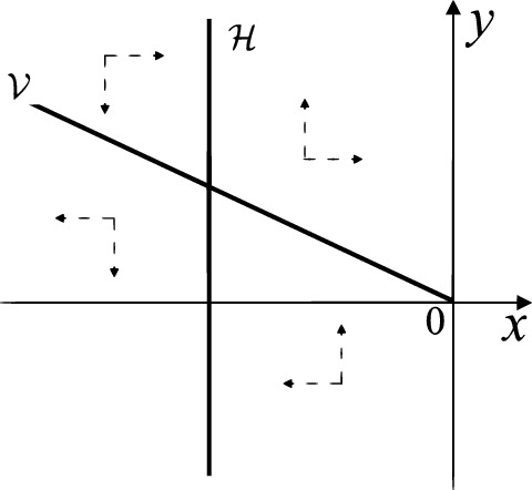
On the other hand for systems there are the horizontal isocline and the vertical isocline . More concretely, we see on the right hand side of , and on the left hand side of . And we get in the upper of , and in the lower of . So in the four regions divided by and , the vector fields are shown in Figs. 2, 3, 4, 5, 6 and 7. Then one branch of the unstable manifold of the saddle intersects the positive y-axis at , while one branch of the stable y-axis at . Then . Solving the equation , i.e.
we get
Note that some orbits of systems intersect y-axis and are symmetric with respect to the x-axis. Let . Then . Thus on the y-axis we look for the values of y such that . Namely
The equality holds when . It implies that there are filled with periodic orbits inside the homoclinic orbit connecting to , seeing Fig. 3. If then . One branch of the stable manifold of goes around the periodic orbit . If then . One branch of the unstable manifold of goes around the periodic orbit . See Figs. 2 and 4.
Fig. 2.
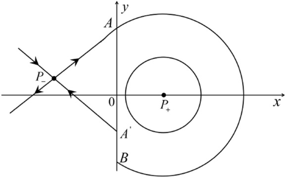
Fig. 3.
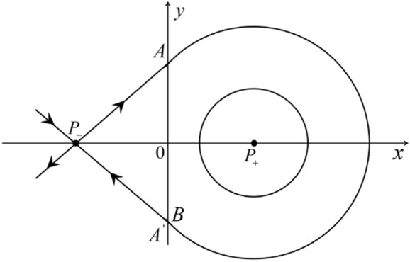
Fig. 4.

Fig. 5.

Fig. 6.

Fig. 7.
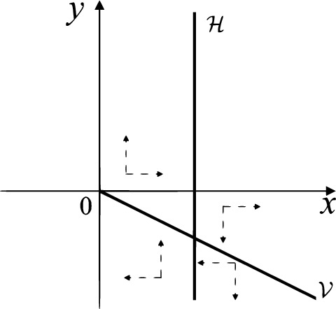
When and either or the equilibrium point is either an unstable node or a stable node. On the other hand for systems there are the horizontal isocline and the vertical isocline . More concretely, we see on the right hand side of , and on the left hand side of . And we get in the upper of , and in the lower of . So we see the vector fields in the four regions divided by and shown in Figs. 8, 9, and 10. There is an orbit linking with the infinity in the half plane . Thus there is no periodic orbits in the half plane .
Fig. 8.
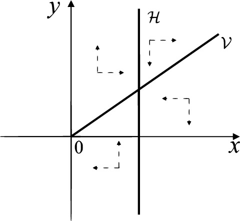
Fig. 9.
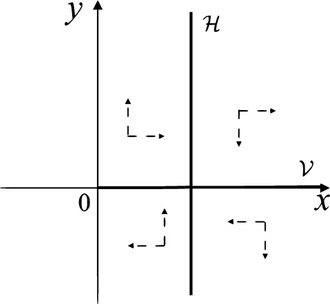
Fig. 10.
When and let (respectively ) be the intersection point of the unstable (respectively stable) manifold of the saddle with the y-axis. Denote by (respectively ) the intersection point of the x-axis with the orbit starting at M (respectively N) if they intersect. When we have the orbits living on the curves for , being symmetry with respect to x-axis. Then the points and exist with . For being small enough we see that is a stable focus and still holds as . It follows from the Poincaré–Bendixson Theorem that there exists periodic orbits in the region surrounded by . Furthermore we claim that there exists a value such that . This means that there exists a homoclinic orbit at and surrounding . In fact when we write the differential systems in the local charts and . Then in the local chart systems write
| 16 |
and in the local chart become
Then there is only one infinite equilibrium point of systems in the local chart , namely and the origin O of the local chart is not an infinite equilibrium point. The eigenvalues of the equilibrium point p are 0 and 1. Therefore by [5, Theorem 2.19] the infinite equilibrium point p is a semi-hyperbolic saddle-node. By the direction of vector fields in Fig. 9 we have the stable manifold of intersecting with the y-axis comes from the semi-hyperbolic saddle-node p. While the unstable manifold of intersecting with the y-axis goes to the stale node . They are shown in Figs. 11, 12 and 13. By the continuity of systems (I) in the interval we prove the claim.
Fig. 11.

Fig. 12.

Fig. 13.

We consider the case that and by the analogue method. Let (respectively ) be the intersection point of the x-axis with the orbit starting from M (respectively N) if they intersect. When we see since as . For small enough we see that the inequality still holds. Similarly by the Poincaré–Bendixson Theorem there exist periodic orbits in the region surrounded by . Furthermore we claim that there exists a value such that . This means that there exists a homoclinic orbit at and surrounding . In fact when there is only one infinite equilibrium point of systems in the local chart , namely and the origin O of the local chart is not an infinite equilibrium point. The eigenvalues of the equilibrium point q are 0 and , and therefore the infinite equilibrium point q is a semi-hyperbolic saddle-node. By the directions of the vector field in Fig. 10 we have that the stable manifold of intersecting the y-axis comes from the semi-hyperbolic saddle-node q. While the unstable manifold of intersects the y-axis and goes to the stable node . They are shown in Figs. 14, 15 and 16. This competes the proof of systems (I).
Fig. 14.
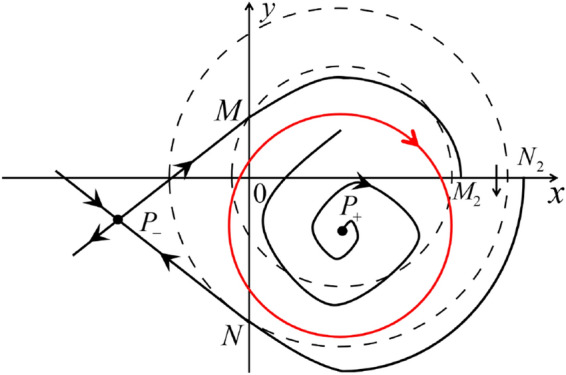
Fig. 15.

Fig. 16.

For systems (II) we see that the differential systems (respectively ) have the equilibrium point (respectively ). Namely . Then the equilibrium point P is real for both systems and . The eigenvalues of the equilibrium point are and . Clearly, , implying that is a saddle. Clearly there is no periodic orbits for systems (II).
For systems (III) the differential systems have the equilibrium point , while the differential systems have the equilibrium point . Then the equilibrium point (respectively ) is virtual for the differential systems (respectively ). Namely systems (III) have no finite equilibrium points, and therefore there is also no periodic orbits for systems (III).
For systems (IV) note that , otherwise because in the case. Then the differential systems have the equilibrium point While the differential systems have the equilibrium point Moreover the equilibrium point (respectively ) is real for the differential systems (respectively ). The eigenvalues of the equilibrium point are 1 and . So if (respectively ) then is an unstable node (respectively a saddle). The eigenvalues of the equilibrium point are and . Then is a saddle if and a stable node if . Clearly there is also no periodic orbits for systems (IV).
For systems (V) we check that systems (respectively ) of systems (V) have an equilibrium point (respectively ). Moreover they are both virtual, and therefore there is no periodic orbits for systems (V).
For systems (VI) we have that the differential systems (respectively ) have the equilibrium point (respectively ). Namely . Then the equilibrium point P is real for both systems and . The eigenvalues of the equilibrium point are 1 and . So if (respectively ) then is an unstable node (respectively a saddle). The eigenvalues of the equilibrium point are and . Then is a saddle if and a stable node if . Thus there is no periodic orbits for systems (VI) and therefore the proof is completed.
Phase Portraits in the Poincaré Disc of Systems (I)
The Finite and Infinite Equilibrium Points
From the proof of Lemma 3 we obtain the results of the finite equilibrium points for systems (I).
For the infinite equilibrium points we write the differential systems in the local charts and . Then in the local chart systems write
| 17 |
and in the local chart become
We separate the study of the infinite equilibrium points of systems in three cases.
Case (I): or . Then there are only two infinite equilibrium points of systems in the local chart , namely and the origin of the local chart is not an infinite equilibrium point.
The eigenvalues of the equilibrium point are and . If then , implying that is a stable node, and if then , implying that is a saddle.
The eigenvalues of the equilibrium point are and . If then , implying that is a saddle, and if then , implying that is an unstable node.
Case (I): and . Then there is only one infinite equilibrium point of systems in the local chart , namely and the origin O of the local chart is not an infinite equilibrium point. The eigenvalues of the equilibrium point p are 0 and . Therefore by [5, Theorem 2.19] the infinite equilibrium point p is a semi-hyperbolic saddle-node.
Case (I): . Then systems have no infinite equilibrium points in the local chart and at the origin of the local chart .
Again we write the differential systems in the local charts and . Then in the local chart systems write
| 18 |
and in the local chart become
As we did for the systems there are only two infinite equilibrium points of systems in the local chart , namely and the origin of the local chart is not an infinite equilibrium point.
The eigenvalues of the equilibrium point are and . Clearly , implying that is a stable node. The eigenvalues of the equilibrium point are and , therefore is an unstable node since .
In summary from the above discussion, we obtain the results of Table 2.
Table 2.
The local phase portraits at the finite and infinite equilibrium points of the continuous piecewise differential systems (I)
| Systems | Conditions | Finite equilibrium points | Infinite equilibrium points |
|---|---|---|---|
| (I) | (I-1): | (stable node) | (saddle) |
| (unstable node) | |||
| (saddle) | (stable node) | ||
| (unstable node) | |||
| (I-2): | (stable node) | p(semi-hyperbolic saddle-node) | |
| (saddle) | (stable node) | ||
| (unstable node) | |||
| (I-3): | (stable focus) | ||
| (saddle) | (stable node) | ||
| (unstable node) | |||
| (I-4): | (center) | ||
| (saddle) | (stable node) | ||
| (unstable node) | |||
| (I-5): | (unstable focus) | ||
| (saddle) | (stable node) | ||
| (unstable node) | |||
| (I-6): | (unstable node) | p(semi-hyperbolic saddle-node) | |
| (saddle) | (stable node) | ||
| (unstable node) | |||
| (I-7): | (unstable node) | (stable node) | |
| (saddle) | |||
| (saddle) | (stable node) | ||
| (unstable node) |
The Global Phase Portraits in the Poincaré Disc
We below give a discussion for passing from the local phase portraits from all the finite and infinite equilibrium points to the global phase portraits in the Poincaré disc.
Note by (17) and (18) that the right hand sides of the equation both have a common factor v, implying that the infinity is invariant, i.e, formed by orbits. Besides we observe that and on the y-axis. Then starting at points lying on the positive y-axis, all orbits go into the half plane while starting at points lying in the negative y-axis, all orbits go into the half plane . According to Table 2 and the direction of the vector fields shown in Figs. 5–10, we below discuss the global phase portraits in the following cases.
In the case (I-1) one stable separatrix of the saddle comes from the unstable node and the second stable separatrix of comes from the unstable node . One unstable separatrix of goes to the stable node and the second unstable separatrix of goes to the stable node . An unstable separatrix of the saddle goes to the stable node . The remaining orbits of the phase portrait are determined where they start and where they end by the type of stability of the equilibrium points and by the Poincaré–Bendixson theorem (see for instance Theorem 1.25 of [1]). Thus the global phase portrait is given in Fig. 17.
Fig. 17.

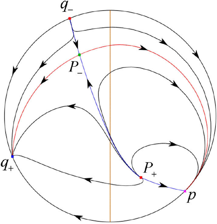
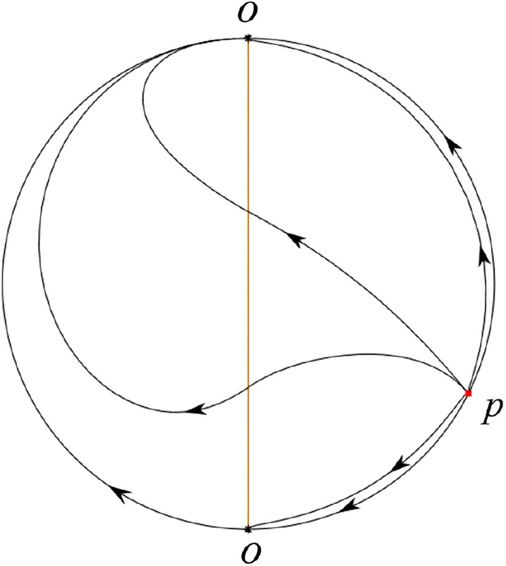
In the case (I-2) one stable separatrix of the saddle comes from the unstable node and the second stable separatrix of comes from the semi-hyperbolic saddle-node p. One unstable separatrix of goes to the stable node and the second unstable separatrix of goes to the stable node . An unstable separatrix of the saddle-node p goes to the stable node . The remaining orbits of the phase portrait are determined where they start and where they end by the type of stability of the equilibrium points and by the Poincaré–Bendixson theorem. Thus the global phase portrait is given in Fig. 18.
Fig. 18.
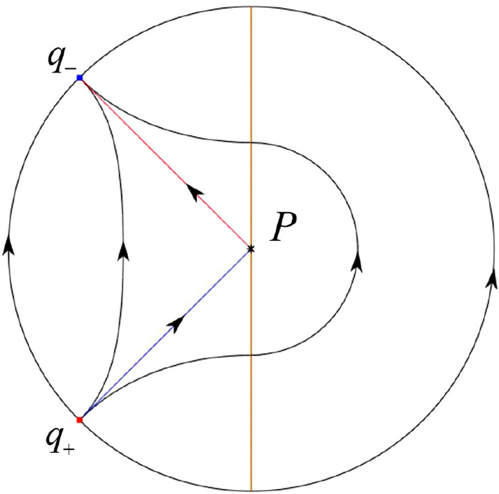
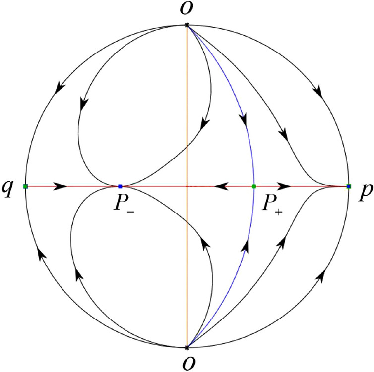
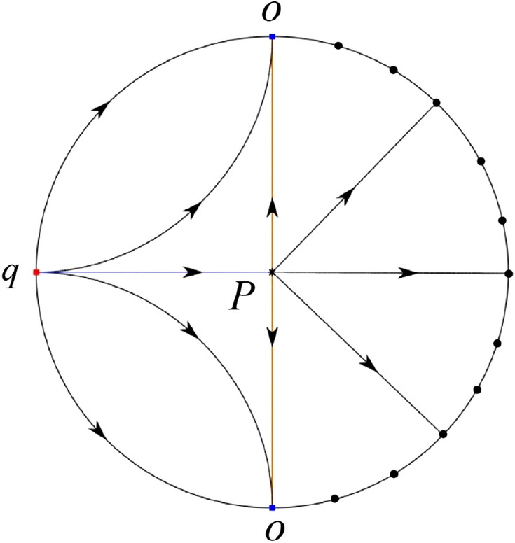
In the case (I-3) two stable separatrices of the saddle come from the unstable node . One unstable separatrix of goes to the stable node and the second unstable separatrix of goes to the stable node . The remaining orbits of the phase portrait are determined by the type of stability of the equilibrium points and by the Poincaré–Bendixson theorem. Thus the global phase portrait is given in Fig. 19,
Fig. 19.
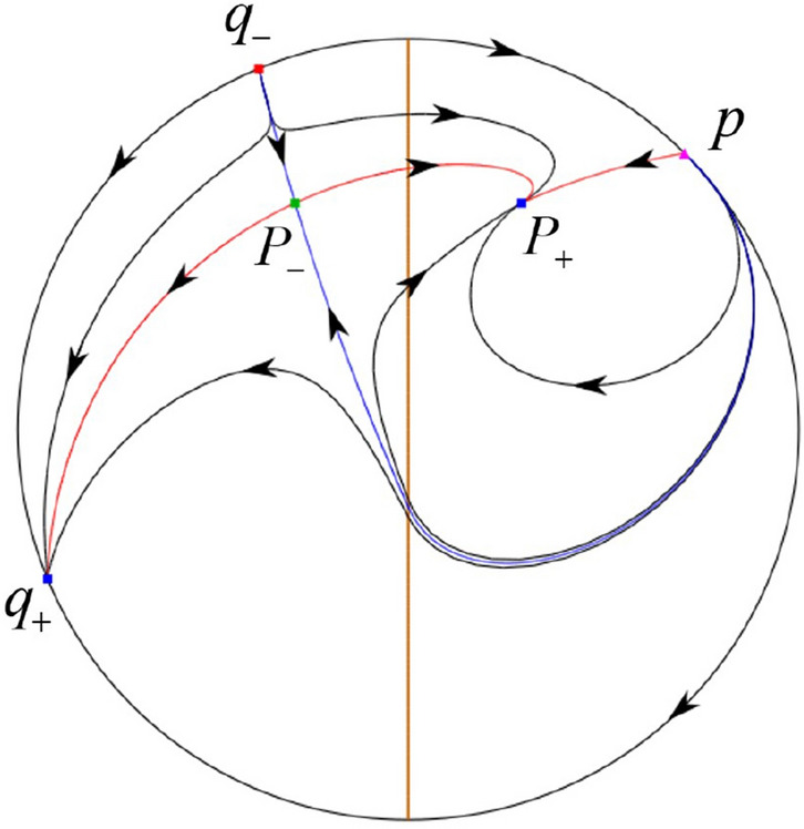
In the case (I-4) one unstable separatrix of the saddle goes to the stable node . One stable separatrix of comes from the unstable node . Then discussions are divided into seven subcases.
-
(i)
The third separatrix of is a homoclinic orbit at .
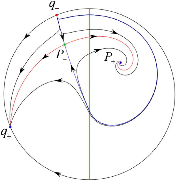
-
(ii)
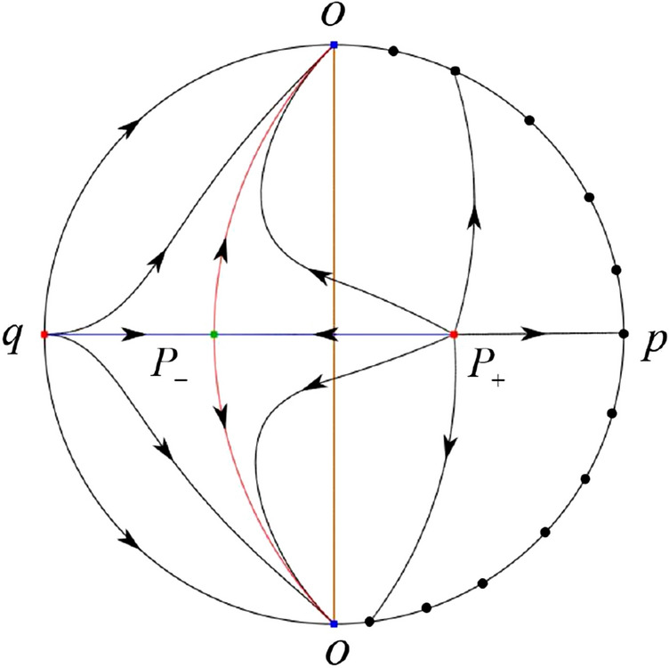
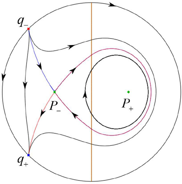
The second unstable separatrix of the saddle goes to and the second stable separatrix of comes from a limit cycle in the strip . The limit cycle is also a separatrix.
-
(iii)
The second unstable separatrix of goes to and the second stable separatrix of comes from the periodic orbit .
-
(iv)
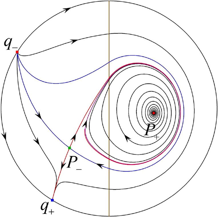
The third separatrix of is a homoclinic orbit at . On the other hand the periodic obit close to the homoclinic orbit is also a separatrix.
-
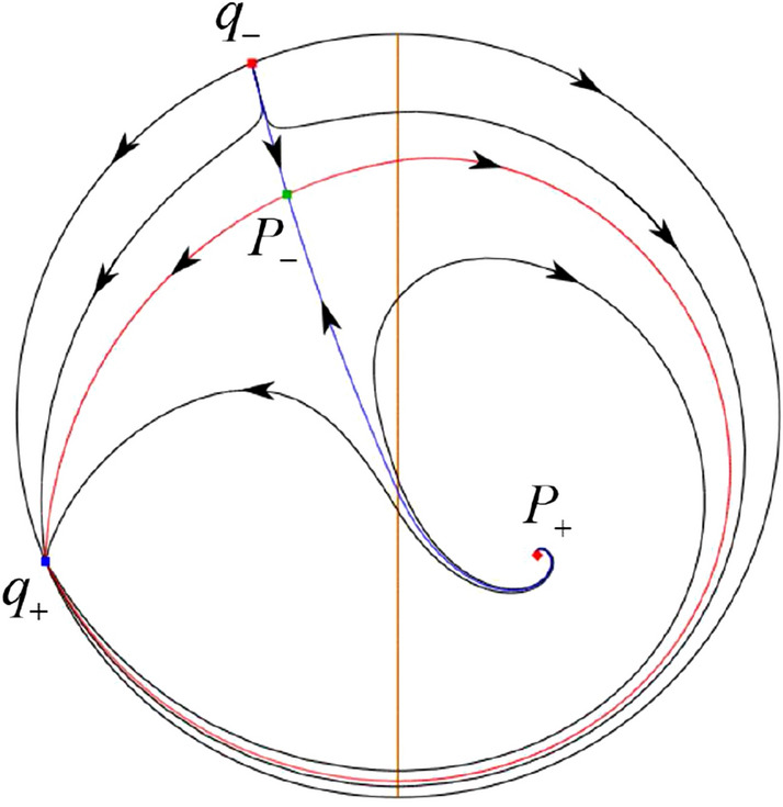
(v)
The second unstable separatrix of goes around a periodic orbit and the second stable separatrix of comes from .
-
(vi)
The second unstable separatrix of goes around a limit cycle. The limit cycle is also a separatrix. The second stable separatrix of comes from .
-
(vii)
The third separatrix of is a homoclinic orbit at . The remaining orbits are determined by the Poincaré–Bendixson theorem and by the type of stability of the equilibrium points. Thus the global phase portraits of the seven subcases are shown in Figs. 20–26, respectively.
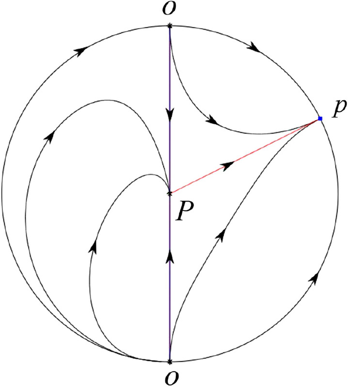
In the case (I-5) one stable separatrix of the saddle comes from the unstable node and the second stable separatrix of comes from the unstable node . Two unstable separatrices of go to the stable node . By the Poincaré–Bendixson theorem and by the type of stability of the equilibrium points we see where the remaining orbits of the phase portrait start and end. Thus the global phase portrait is given in Fig. 27.
Fig. 20.
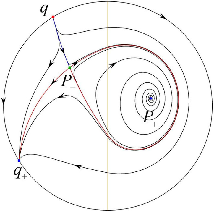
Fig. 26.
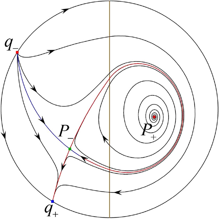
Fig. 27.
In the case (I-6) one stable separatrix of the saddle comes from the unstable node and the second stable separatrix of comes from the unstable node . One unstable separatrix of goes to the stable node and the second unstable separatrix of goes to the semi-hyperbolic saddle-node p. A stable separatrix of the saddle-node p comes from the unstable node . We determine the remaining orbits of the phase portrait by the Poincaré–Bendixson theorem and by the type of stability of the equilibrium points. Thus the global phase portrait is shown in Fig. 28.
Fig. 28.
In the case (I-7) one stable separatrix of the saddle comes from the unstable node and the second stable separatrix of comes from the unstable node . One unstable separatrix of goes to the stable node and the second unstable separatrix of goes to the stable node . An stable separatrix of the saddle comes from . By the Poincaré–Bendixson theorem and by the type of stability of the equilibrium points we get the remaining orbits of the phase portrait. Thus the global phase portrait is given in Fig. 29.
Fig. 29.

Phase Portraits in the Poincaré Disc of Systems (II)
The Finite and Infinite Equilibrium Points
As it is given in the proof of Lemma 3 the differential systems and have the same real equilibrium point P(0, 0) and P is a saddle for systems .
For systems the eigenvalues of P are and . So if (respectively ) then (respectively ), implying that P is a stable (respectively an unstable) node. If (respectively ) then are a pair of imaginary eigenvalues with negative (respectively positive) real part, implying that P is a stable (respectively an unstable) focus. If then are a pair of purely imaginary eigenvalues, implying that P is a center.
For the infinite equilibrium points we write the differential systems in the local charts and . Then in the local chart systems write
| 19 |
and in the local chart become
We separate the study of the infinite equilibrium points of systems in three cases.
Case (II): or . Then there are only two infinite equilibrium points of systems in the local chart , namely and the origin of the local chart is not an infinite equilibrium point.
The eigenvalues of the equilibrium point are and . If then , implying that is a saddle, and if then , implying that is an unstable node.
The eigenvalues of the equilibrium point are and . If then , implying that is a stable node, and if then , implying that is a saddle.
Case (II): and . Then there is only one infinite equilibrium point of systems in the local chart , namely and the origin O of the local chart is not an infinite equilibrium point. The eigenvalues of the equilibrium point p are 0 and . Therefore by [5, Theorem 2.19] the infinite equilibrium point p is a semi-hyperbolic saddle-node.
Case (II): . Then systems have no infinite equilibrium points in the local chart and at the origin of the local chart .
Again we write the differential systems in the local charts and . Then in the local chart systems write
| 20 |
and in the local chart become
As we did for the systems there are only two infinite equilibrium points of systems in the local chart , namely and the origin of the local chart is not an infinite equilibrium point.
The eigenvalues of the equilibrium point are and . Clearly, , implying that is an unstable node. The eigenvalues of the equilibrium point are and , therefore is a stable node since .
In summary from the above discussion, we obtain the results of Table 3.
Table 3.
The local phase portraits at the finite and infinite equilibrium points of the continuous piecewise differential systems (II)
| Systems | Conditions | Finite equilibrium points | Infinite equilibrium points |
|---|---|---|---|
| (II) | (II-1): | P(stable node) | (unstable node) |
| (saddle) | |||
| P(saddle) | (unstable node) | ||
| (stable node) | |||
| (II-2): | P(stable node) | p(semi-hyperbolic saddle-node) | |
| P(saddle) | (unstable node) | ||
| (stable node) | |||
| (II-3): | P(stable focus) | ||
| P(saddle) | (unstable node) | ||
| (stable node) | |||
| (II-4): | P(center) | ||
| P(saddle) | (unstable node) | ||
| (stable node) | |||
| (II-5): | P(unstable focus) | ||
| P(saddle) | (unstable node) | ||
| (stable node) | |||
| (II-6): | P(unstable node) | p(semi-hyperbolic saddle-node) | |
| P(saddle) | (unstable node) | ||
| (stable node) | |||
| (II-7): | P(unstable node) | (saddle) | |
| (stable node) | |||
| P(saddle) | (unstable node) | ||
| (stable node) |
The Global Phase Portraits in the Poincaré Disc
Similar to systems (I), by (19) and (20) we see that the right hand sides of the equation both have a common factor v, implying that the infinity is formed by orbits. Further check that and on the y-axis. Then starting at points lying on the positive y-axis, all orbits go into the half plane while starting at points lying in the negative y-axis, all orbits go into the half plane . On the other hand for systems there are the horizontal isocline and the vertical isocline . Also for systems (19) there are two invariant lines , and for systems (20) there are two invariant lines . According to Table 3 we below discuss the global phase portraits in the following cases.
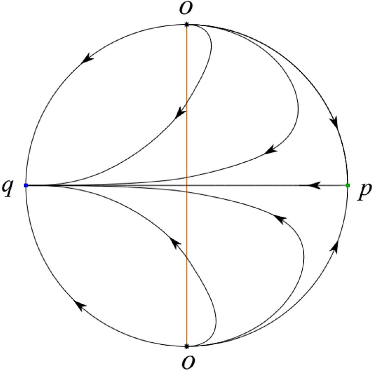
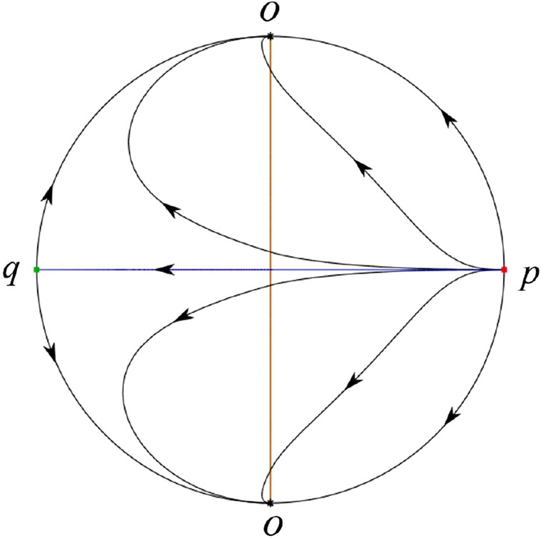
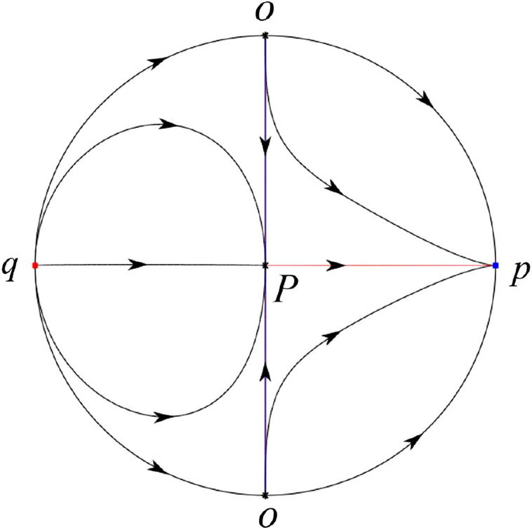
In the case (II-1) two separatrices respectively lying on the line and are the orbits at the boundary of a hyperbolic sector at P. One stable separatrix of the saddle P in the half plane comes from the unstable node lying on the line . One unstable separatrix of the saddle lying on the line goes to the stable node P in the half plane . The remaining orbits of the phase portrait are determined where they start and where they end by the type of stability of the equilibrium points and by the Poincaré–Bendixson theorem. Thus the global phase portrait is shown in Fig. 30.
Fig. 30.
Note that for the remain cases (II-2)–(II-7) the phase portrait is the same as the case (II-1) in the half plane . In the half plane the phase portrait is studied in what follows.
In the case (II-2) one unstable separatrix of the saddle-node p goes to the stable node P in the half plane , which lies on the line . The remaining orbits of the phase portrait are determined by the type of stability of the equilibrium points and by the Poincaré–Bendixson theorem. Thus the global phase portrait is shown in Fig. 31.
Fig. 31.

In cases (II-3)–(II-5) there is no separatrices in the half plane . The remaining orbits of the phase portrait are determined by the type of stability of the equilibrium points and by the Poincaré–Bendixson theorem. Thus the global phase portraits of these three cases are given in Fig. 32.
Fig. 32.
In the case (II-6) one stable separatrix of the saddle-node p comes from the unstable node P in the half plane lying on the line . We get the remaining orbits of the phase portrait by the type of stability of the equilibrium points and by the Poincaré–Bendixson theorem. Thus the global phase portrait is shown in Fig. 33.
Fig. 33.

In the case (II-7) a separatrix is one of the orbits at the boundary of a hyperbolic sector at P lying on the line in the half plane . One stable separatrix of the saddle comes from the unstable node P in the half plane lying on the line . We get the remaining orbits of the phase portrait by the type of stability of the equilibrium points and by the Poincaré–Bendixson theorem. Thus the global phase portrait is shown in Fig. 34.
Fig. 34.
Phase Portraits in the Poincaré Disc of Systems (III)
The Finite and Infinite Equilibrium Points
As it is given in the proof of Lemma 3 the differential systems have the virtual equilibrium point , while the differential systems have the virtual equilibrium point .
Doing the change , systems (III) become
Systems are the same that systems of systems (I), while systems are the same that systems of systems (I). So from the results of systems (I) for the finite and infinite equilibrium points of systems (III) we get Table 4.
Table 4.
The local phase portraits at the finite and infinite equilibrium points of the continuous piecewise differential systems (III)
| Systems | Conditions | Finite equilibrium points | Infinite equilibrium points |
|---|---|---|---|
| (III) | (III-1): | (stable node) | (unstable node) |
| (saddle) | |||
| (saddle) | (unstable node) | ||
| (stable node) | |||
| (III-2): | (stable node) | p(semi-hyperbolic saddle-node) | |
| (saddle) | (unstable node) | ||
| (stable node) | |||
| (III-3): | (stable focus) | ||
| (saddle) | (unstable node) | ||
| (stable node) | |||
| (III-4): | (center) | ||
| (saddle) | (unstable node) | ||
| (stable node) | |||
| (III-5): | (unstable focus) | ||
| (saddle) | (unstable node) | ||
| (stable node) | |||
| (III-6): | (unstable node) | p(semi-hyperbolic saddle-node) | |
| (saddle) | (unstable node) | ||
| (stable node) | |||
| (III-7): | (unstable node) | (saddle) | |
| (stable node) | |||
| (saddle) | (unstable node) | ||
| (stable node) |
The Global Phase Portraits in the Poincaré Disc
Similar to systems (I) we check and on the y-axis. Then starting at points lying on the positive y-axis all orbits go into the half plane , while starting at points lying in the negative y-axis all orbits go into the half plane . On the other hand the infinity is formed by orbits. According to Table 4 we below discuss the global phase portraits in the following cases.
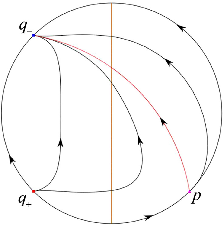
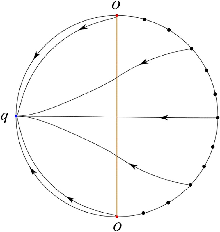
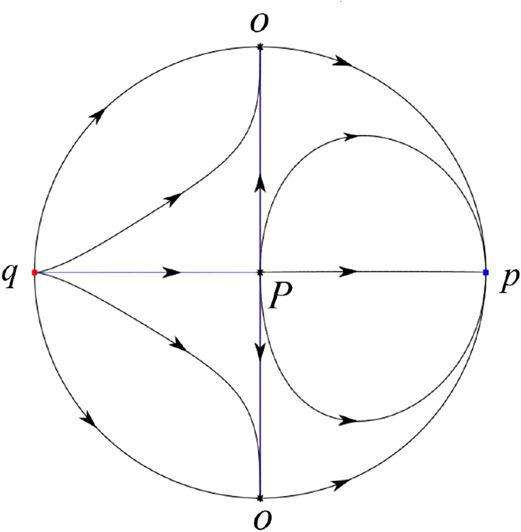
In the case (III-1) an unstable separatrix of the saddle goes to the stable node . The remaining orbits of the phase portrait are determined where they start and where they end by the type of stability of the equilibrium points and by the Poincaré–Bendixson theorem. Thus the global phase portrait is given in Fig. 35.
Fig. 35.

In the case (III-2) an unstable separatrix of the saddle-node p goes to the stable node . By the type of stability of the equilibrium points and by the Poincaré–Bendixson theorem we get the remaining orbits of the phase portrait. Thus the global phase portrait is given in Fig. 36.
Fig. 36.
In the case (III-3)–(III-5) there is no separatrices in the phase portrait. All orbits leave for . Thus the global phase portrait is shown in Fig. 37.
Fig. 37.

In the case (III-6) a stable separatrix of the saddle-node p comes from the unstable node . The remaining orbits of the phase portrait are determined by the type of stability of the equilibrium points and by the Poincaré–Bendixson theorem. Thus the global phase portrait is shown in Fig. 38.
Fig. 38.

In the case (III-7) a stable separatrix of the saddle comes from the unstable node . Similarly we get the remaining orbits of the phase portrait. Thus the global phase portrait is shown in Fig. 39.
Fig. 39.
Phase Portraits in the Poincaré Disc of Systems (IV)
The Finite and Infinite Equilibrium Points
From the proof of Lemma 3 we obtain the results of the finite equilibrium points for systems (IV).
For the infinite equilibrium points we write the differential systems in the local charts and they become
| 21 |
and in the local chart they become
We separate the study of the infinite equilibrium points of systems in two cases.
Case (IV): . Then there is only one infinite equilibrium point of systems in the local chart , namely and the origin O of the local chart is an infinite equilibrium point. The eigenvalues of the equilibrium point p are and . Thus p is a stable node if and a saddle if . The eigenvalues of the equilibrium point O are and . Then O is an unstable node if , a semi-hyperbolic saddle-node if , a saddle if , and a stable node .
Case (IV): . We consider two subcases: and . In the first subcase there is no infinite equilibrium point in the local chart , but the origin O of the local chart is an infinite equilibrium point. Moreover the eigenvalues of O are 0 and , implying that it is a semi-hyperbolic saddle-node. In the second subcase all points on the u-axis are infinite equilibrium points in the local chart for systems . Since the eigenvalues at each one of these equilibrium points are 0 and , by the normally hyperbolic equilibrium points theorem (see [8]) it follows that at each one of these equilibrium points ends an orbit. The origin of the local chart is also an equilibrium point inside the continuum of equilibrium points at infinity with eigenvalues 0 and , so the same conclusion for it.
Again we write the differential systems in the local charts and . Then in the local chart systems write
| 22 |
and in the local chart become
As we did for the systems we separate the study of the infinite equilibrium points of systems in two cases.
Case (IV): . Then there is only one infinite equilibrium point of systems in the local chart , namely and the origin O of the local chart is an infinite equilibrium point. The eigenvalues of the equilibrium point q are 1 and . Then q is a saddle if and an unstable node if . The eigenvalues of the equilibrium point O are and . Then O is an unstable node if , a saddle if , a semi-hyperbolic saddle-node if and a stable node .
Case (IV): . Again we consider two subcases: and . In the first subcase there is no infinite equilibrium point in the local chart , but the origin O of the local chart is an infinite equilibrium point. Moreover the eigenvalues of O are 0 and 1, implying that it is a semi-hyperbolic saddle-node. In the second subcase all points on the u-axis are infinite equilibrium points in the local chart for systems . Since the eigenvalues at each one of these equilibrium points are 0 and , by the normally hyperbolic equilibrium points theorem at each one of these equilibrium points starts an orbit. At the origin of the local chart we also have a semi-hyperbolic saddle-node.
In summary from the above discussion, we obtain the results of Table 5.
Table 5.
The local phase portraits at the finite and infinite equilibrium points of the continuous piecewise differential systems (IV)
| Systems | Conditions | Finite equilibrium points | Infinite equilibrium points |
|---|---|---|---|
| (IV) | (IV-1): | (saddle) | p(stable node) |
| O(unstable node) | |||
| (stable node) | q(saddle) | ||
| O(unstable node) | |||
| (IV-2): , | (saddle) | p(stable node) | |
| O(unstable node) | |||
| (stable node) | |||
| O(semi-hyperbolic saddle-node) | |||
| (IV-3): | (saddle) | p(stable node) | |
| O(unstable node) | |||
| (stable node) | u-axis(starts an orbit) | ||
| O(starts an orbit) | |||
| (IV-4): | (saddle) | p(stable node) | |
| O(unstable node) | |||
| (stable node) | |||
| O(semi-hyperbolic saddle-node) | |||
| (IV-5): | (saddle) | p(stable node) | |
| O(unstable node) | |||
| (stable node) | q(unstable node) | ||
| O(saddle) | |||
| (IV-6): | (unstable node) | p(stable node) | |
| O(saddle) | |||
| (saddle) | q(unstable node) | ||
| O(stable node) | |||
| (IV-7): | (unstable node) | ||
| O(semi-hyperbolic saddle-node) | |||
| (saddle) | q(unstable node) | ||
| O(stable node) | |||
| (IV-8): | (unstable node) | u-axis(ends an orbit) | |
| O(ends an orbit) | |||
| (saddle) | q(unstable node) | ||
| O(stable node) | |||
| (IV-9): | (unstable node) | ||
| O(semi-hyperbolic saddle-node) | |||
| (saddle) | q(unstable node) | ||
| O(stable node) | |||
| (IV-10): | (unstable node) | p(saddle) | |
| O(stable node) | |||
| (saddle) | q(unstable node) | ||
| O(stable node) |
The Global Phase Portraits in the Poincaré Disc
First we see on the y-axis. Then starting at points lying on the y-axis all orbits go into the half plane . On the other hand the infinity as always is formed by orbits because the equations of equations (21) and (22) have a common factor v. According to Table 5 we divide the study of the global phase portraits in the following cases.
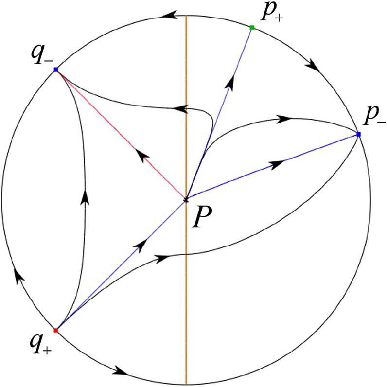
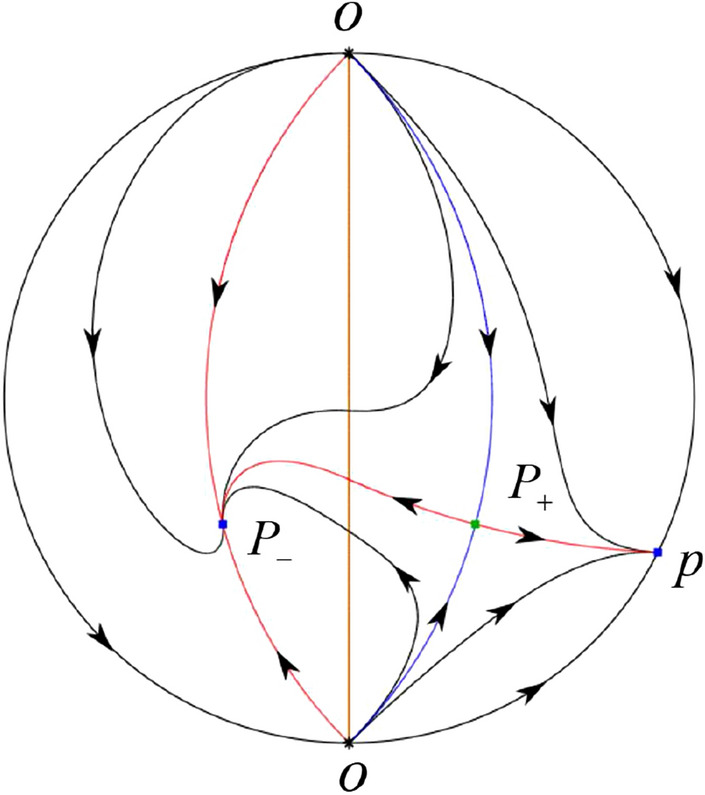
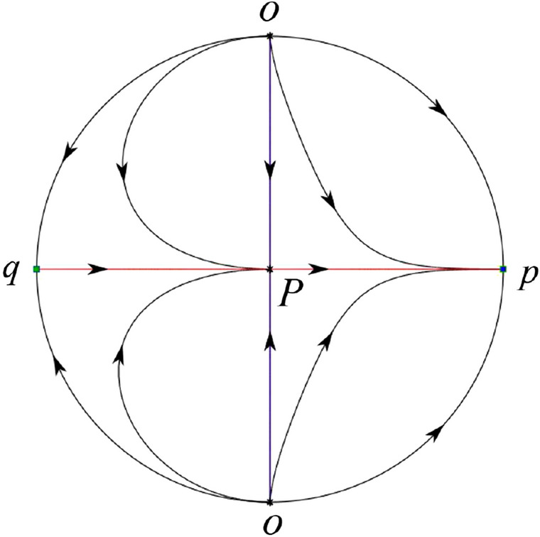
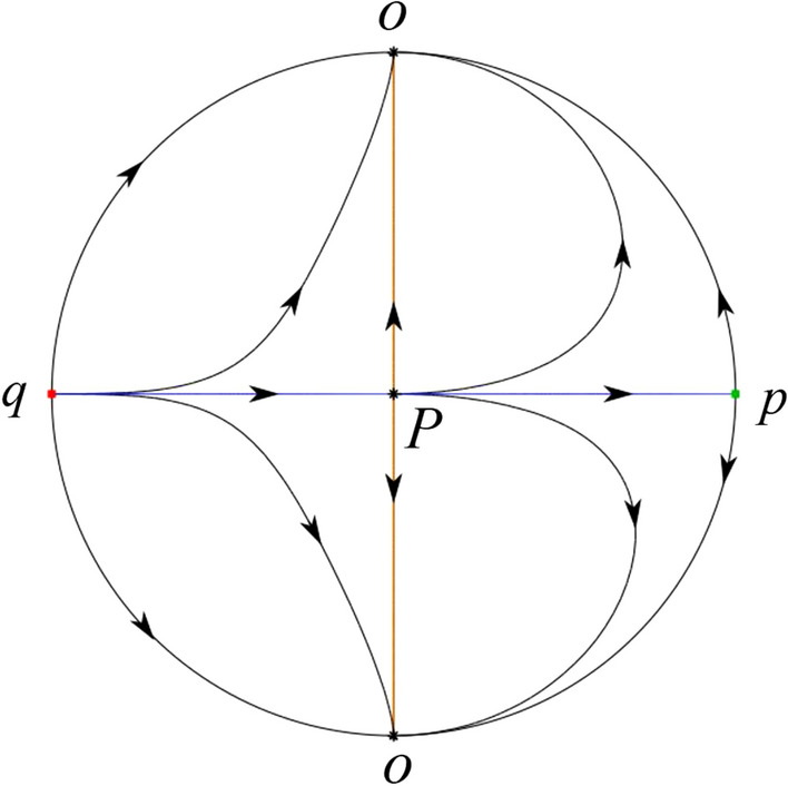
In the case (IV-1) one stable separatrix of the saddle comes from the unstable node O in the positive y-direction and the second stable separatrix of comes from the unstable node O in the negative y-direction. One unstable separatrix of goes to the stable node p and the second unstable separatrix of goes to the stable node . An unstable separatrix of the saddle q goes to . The remaining orbits of the phase portrait are determined where they start and they end by the type of stability of the equilibrium points and by the Poincaré–Bendixson theorem. Thus the global phase portrait is shown in Fig. 40.
Fig. 40.
In the case (IV-2) one stable separatrix of the saddle comes from the semi-hyperbolic saddle-node O in the positive y-direction and the second stable separatrix of comes from the unstable node O in the negative y-direction. One unstable separatrix of goes to the stable node p and the second unstable separatrix of goes to the stable node . The remaining orbits of the phase portrait are determined by the type of stability of the equilibrium points and by the Poincaré–Bendixson theorem. Thus the global phase portrait is shown in Fig. 41.
Fig. 41.
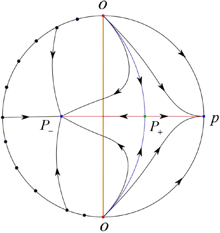
In the case (IV-3) one stable separatrix of the saddle comes from the unstable node O in the positive y-direction of the half plane and the second stable separatrix of comes from the equilibrium point O in the negative y-direction of the half plane . One unstable separatrix of goes to the stable node p and the second unstable separatrix of goes to the stable node . The infinity of is filled with equilibrium points. At each one of these infinite equilibrium points starts an orbit going to . The remaining orbits of the phase portrait are determined by the type of stability of the equilibrium points and by the Poincaré–Bendixson theorem. Thus the global phase portrait is shown in Fig. 42.
Fig. 42.
In the case (IV-4) one stable separatrix of the saddle comes from the unstable node O in the positive y-direction in the half plane and the second stable separatrix of comes from the unstable node O in the negative y-direction. One unstable separatrix of goes to the stable node p and the second unstable separatrix of goes to the stable node . An unstable separatrix of the saddle-node O in the positive y-direction goes to the stable node . The remaining orbits of the phase portrait are determined by the type of stability of the equilibrium points and by the Poincaré–Bendixson theorem. Thus the global phase portrait is shown in Fig. 43.
Fig. 43.

In the case (IV-5) one stable separatrix of the saddle comes from the saddle-node O in the positive y-direction and the second stable separatrix of comes from the saddle-node O in the negative y-direction. An unstable separatrix of goes to the stable node p and the second unstable separatrix of goes to the stable node . One unstable separatrix of the saddle-node O in the positive y-direction goes to the stable node and an unstable separatrix of the saddle-node O in the negative y-direction goes to . By the type of stability of the equilibrium point and by the Poincaré–Bendixson theorem we get the remaining orbits of the phase portrait. Thus the global phase portrait is shown in Fig. 44.
Fig. 44.

In the case (IV-6) one stable separatrix of the saddle comes from the unstable node q and the second stable separatrix of comes from the unstable node . One unstable separatrix of goes to the saddle-node O in the positive y-direction and the second unstable separatrix of goes to the saddle-node O in the negative y-direction. A stable separatrix of the saddle-node O in the positive y-direction comes from and a stable separatrix of the saddle-node O in the negative y-direction comes from . Similarly we get the remaining orbits of the phase portrait by the type of stability of the equilibrium points and by the Poincaré–Bendixson theorem. Thus the global phase portrait is shown in Fig. 45.
Fig. 45.
In the case (IV-7) one stable separatrix of the saddle comes from the unstable node q and the second stable separatrix of comes from the unstable node . One unstable separatrix of goes to the saddle-node O in the positive y-direction of the half plane and the second unstable separatrix of goes to the stable node O in the negative y-direction. An stable separatrix of the saddle-node O in the positive y-direction comes from . The remaining orbits of the phase portrait are determined by the type of stability of the equilibrium points and by the Poincaré–Bendixson theorem. Thus the global phase portrait is shown in Fig. 46.
Fig. 46.

In the case (IV-8) one stable separatrix of the saddle comes from the unstable node q and the second stable separatrix of comes from the unstable node . One unstable separatrix of goes to the stable node O in the positive y-direction of the half plane and the second unstable separatrix of goes to the stable node O in the negative y-direction of the half plane . The infinity of is filled with equilibrium points. At each one of these infinite equilibrium points arrives an orbit starting at . The remaining orbits of the phase portrait are determined by the type of stability of the equilibrium points and by the Poincaré–Bendixson theorem. Thus the global phase portrait is shown in Fig. 47.
Fig. 47.
In the case (IV-9) one stable separatrix of the saddle comes from the unstable node q and the second stable separatrix of comes from the unstable node . One unstable separatrix of goes to the stable node O in the positive y-direction and the second unstable separatrix of goes to the saddle-node O in the negative y-direction. A stable separatrix of the saddle-node O in the negative y-direction comes from . Similar to the above, we get the remaining orbits of phase portrait. Thus the global phase portrait is shown in Fig. 48.
Fig. 48.

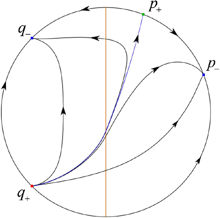
In the case (IV-10) one stable separatrix of the saddle comes from the unstable node q and the second stable separatrix of comes from the unstable node . One unstable separatrix of goes to the stable node O in the positive y-direction and the second unstable separatrix of goes to the stable node O in the negative y-direction. A stable separatrix of the saddle p comes from . Similarly we get the remaining orbits of the phase portrait by the type of stability of the equilibrium points and by the Poincaré–Bendixson theorem. Thus the global phase portrait is shown in Fig. 49.
Fig. 49.

Phase Portraits in the Poincaré Disc of Systems (V)
The Finite and Infinite Equilibrium Points
From the proof of Lemma 3 we see that systems have the virtual equilibrium points and systems have the virtual equilibrium point .
Note that systems of systems (V) are the same that systems of systems (IV) if we regard as . While systems of systems (V) are also the same that systems of systems (IV). So from the results of systems (IV) for the finite and infinite equilibrium points of systems (V) we get Table 6.
Table 6.
The local phase portraits at the finite and infinite equilibrium points of the continuous piecewise differential systems (V)
| Systems | Conditions | Finite equilibrium points | Infinite equilibrium points |
|---|---|---|---|
| (V) | (V-1): | (stable node) | p(saddle) |
| O(unstable node) | |||
| (saddle) | q(stable node) | ||
| O(unstable node) | |||
| (V-2): | (stable node) | ||
| O(semi-hyperbolic saddle-node) | |||
| (saddle) | q(stable node) | ||
| O(unstable node) | |||
| (V-3): | (stable node) | u-axis(starts an orbit) | |
| O(starts an orbit) | |||
| (saddle) | q(stable node) | ||
| O(unstable node) | |||
| (V-4): | (stable node) | ||
| O(semi-hyperbolic saddle-node) | |||
| (saddle) | q(stable node) | ||
| O(unstable node) | |||
| (V-5): | (stable node) | p(unstable node) | |
| O(saddle) | |||
| (saddle) | q(stable node) | ||
| O(unstable node) | |||
| (V-6): | (saddle) | p(unstable node) | |
| O(stable node) | |||
| (unstable node) | q(stable node) | ||
| O(saddle) | |||
| (V-7): | (saddle) | p(unstable node) | |
| O(stable node) | |||
| (unstable node) | |||
| O(semi-hyperbolic saddle-node) | |||
| (V-8): | (saddle) | p(unstable node) | |
| O(stable node) | |||
| (unstable node) | u-axis(ends an orbit) | ||
| O(ends an orbit) | |||
| (V-9): | (saddle) | p(unstable node) | |
| O(stable node) | |||
| (unstable node) | |||
| O(semi-hyperbolic saddle-node) | |||
| (V-10): | (saddle) | p(unstable node) | |
| O(stable node) | |||
| (unstable node) | q(saddle) | ||
| O(stable node) |
The Global Phase Portraits in the Poincaré Disc
According to Table 6 we below discuss the global phase portraits in the following cases.
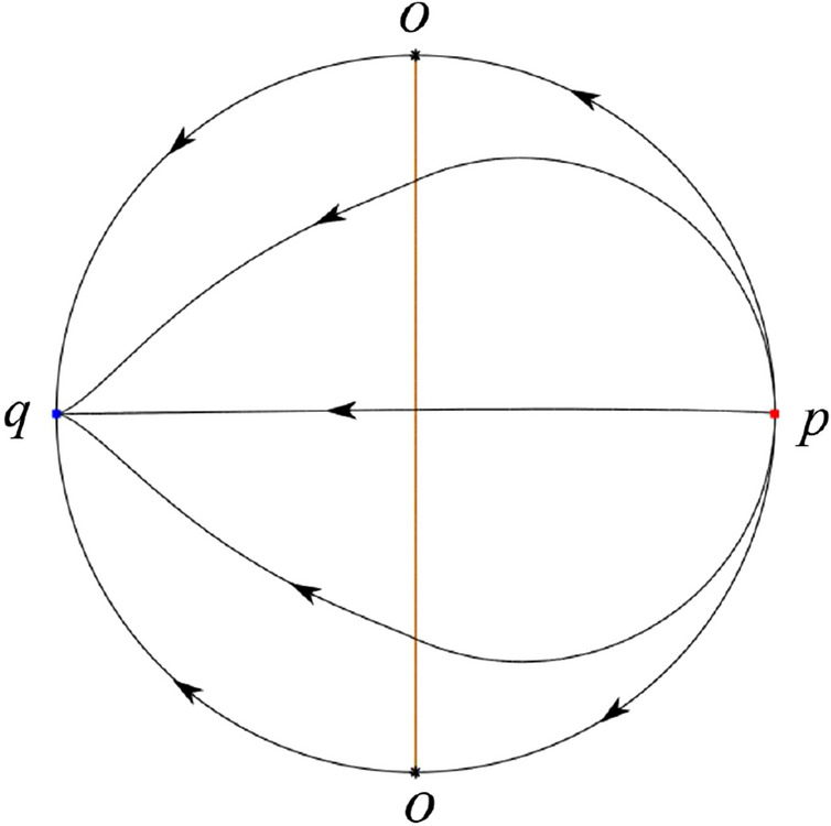
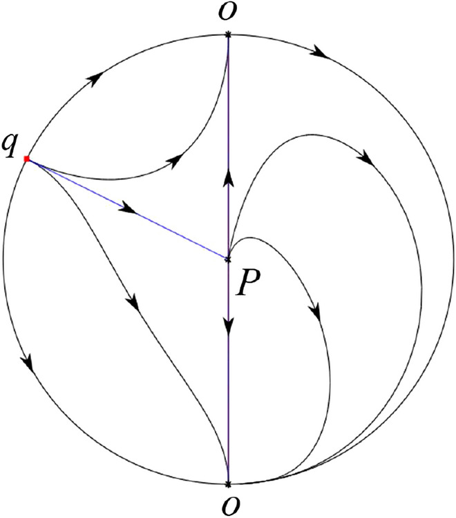
In the case (V-1) an unstable separatrix of the saddle p goes to the stable node q. The remaining orbits of the phase portrait are determined where they start and they end by the type of stability of the equilibrium points and by the Poincaré–Bendixson theorem. Thus the global phase portrait is shown in Fig. 50.
Fig. 50.
In the case (V-2) an unstable separatrix comes from the saddle-node O in the negative y-direction and goes to the stable node q. The remaining orbits of the phase portrait are determined by the type of stability of the equilibrium points and by the Poincaré–Bendixson theorem. Thus the global phase portrait is shown in Fig. 51.
Fig. 51.

In the case (V-3) the infinity of is filled with equilibrium points. At each one of these infinite equilibrium points starts an orbit going to the stable node q. Thus the global phase portrait is shown in Fig. 52.
Fig. 52.
In the case (V-4) an unstable separatrix comes from the saddle-node O in the negative y-direction and goes to the stable node q. We similarly get the remaining orbits of the phase portrait by the type of stability of the equilibrium points and by the Poincaré–Bendixson theorem. Thus the global phase portrait is shown in Fig. 53.
Fig. 53.

In the case (V-5) an unstable separatrix comes from the saddle-node O in the positive y-direction and goes to the stable node q. An unstable separatrix comes from the saddle-node O in the negative y-direction and goes to q. The remaining orbits in the phase portrait are determined by the type of stability of the equilibrium points and by the Poincaré–Bendixson theorem. Thus the global phase portrait is shown in Fig. 54.
Fig. 54.
In the case (V-6) an unstable separatrix comes from the unstable node p and goes to the saddle-node O in the positive y-direction. Another unstable separatrix comes from p and goes to the saddle-node O in the negative y-direction. The remaining orbits in the phase portrait are determined by the type of stability of the equilibrium points and by the Poincaré–Bendixson theorem. Thus the global phase portrait is shown in Fig. 55.
Fig. 55.

In the case (V-7) an unstable separatrix comes from the unstable node p and goes to the saddle-node O in the positive y-direction. We get the remaining orbits by the type of stability of the equilibrium points and by the Poincaré–Bendixson theorem. Thus the global phase portrait is shown in Fig. 56.
Fig. 56.

In the case (V-8) the infinity of the half plane is filled with equilibrium point. At each one of these infinite equilibrium points arrives an orbit starting at the unstable node p. Thus the global phase portrait is shown in Fig. 57.
Fig. 57.

In the case (V-9) an unstable separatrix comes from the unstable node p and goes to the saddle-node O in the negative y-direction. We obtain the remaining orbits by the type of stability of the equilibrium points and by the Poincaré–Bendixson theorem. Thus the global phase portrait is shown in Fig. 58.
Fig. 58.
In the case (V-10) a stable separatrix of the saddle q come from the unstable node p. We similarly get the remaining orbits by the type of stability of the equilibrium points and by the Poincaré–Bendixson theorem. Thus the global phase portrait is shown in Fig. 59.
Fig. 59.
Phase Portraits in the Poincaré Disc of Systems (VI)
The Finite and Infinite Equilibrium Points
As it is given in the proof of Lemma 3 we obtain the results of the finite equilibrium points for systems (VI).
For the infinite equilibrium points we write the differential systems in the local charts and become
and in the local chart become
We separate the study of the infinite equilibrium points of systems in two cases.
Case (VI): . Then there is only one infinite equilibrium point of systems in the local chart , namely and the origin O of the local chart is an infinite equilibrium point. The eigenvalues of the equilibrium point p are and . Thus p is a stable node if , and a saddle if . The eigenvalues of the equilibrium point O are and . Then O is an unstable node if , a semi-hyperbolic saddle-node if , a saddle if and a stable node .
Case (VI): . We consider two subcases: and . In the first subcase there is no infinite equilibrium point in the local chart , but the origin O of the local chart is an infinite equilibrium point. Moreover the eigenvalues of O are 0 and , implying that it is a semi-hyperbolic saddle-node. In the second subcase all points on the u-axis are infinite equilibrium points in the local chart for systems . Since the eigenvalues at each one of these equilibrium points are 0 and , it follows that at each one of these equilibrium points ends an orbit. The origin of the local chart is also an equilibrium point inside the continuum of equilibrium points at infinity with eigenvalues 0 and , so the same conclusion for it.
Again we write the differential systems in the local charts and . Then in the local chart systems write
and in the local chart become
As we did for the systems we separate the study of the infinite equilibrium points of systems in two cases.
Case (VI): . Then there is only one infinite equilibrium point of systems in the local chart , namely and the origin O of the local chart is an infinite equilibrium point. The eigenvalues of the equilibrium point q are 1 and . Then q is a saddle if and an unstable node if . The eigenvalues of the equilibrium point O are and . Then O is an unstable node if , a saddle if , a semi-hyperbolic saddle-node if and a stable node .
Case (VI): . Again we consider two subcases: and . In the first subcase there is no infinite equilibrium point in the local chart , but the origin O of the local chart is an infinite equilibrium point. Moreover the eigenvalues of O are 0 and 1, implying that it is a semi-hyperbolic saddle-node. In the second subcase all points on the u-axis are infinite equilibrium points in the local chart for systems . Since the eigenvalues at each one of these equilibrium points are 0 and , at each one of these equilibrium points starts an orbit. At the origin of the local chart we also have a semi-hyperbolic saddle-node.
In summary from the above discussion, we obtain the results of Table 7.
Table 7.
The local phase portraits at the finite and infinite equilibrium points of the continuous piecewise differential systems (VI)
| Systems | Conditions | Finite equilibrium points | Infinite equilibrium points |
|---|---|---|---|
| (VI) | (VI-1): | P(saddle) | p(stable node) |
| O(unstable node) | |||
| P(stable node) | q(saddle) | ||
| O(unstable node) | |||
| (VI-2): | P(saddle) | p(stable node) | |
| O(unstable node) | |||
| P(stable node) | |||
| O(semi-hyperbolic saddle-node) | |||
| (VI-3): | P(saddle) | p(stable node) | |
| O(unstable node) | |||
| P(stable node) | u-axis(starts an orbit) | ||
| O(starts an orbit) | |||
| (VI-4): | P(saddle) | p(stable node) | |
| O(unstable node) | |||
| P(stable node) | |||
| O(semi-hyperbolic saddle-node) | |||
| (VI-5): | P(saddle) | p(stable node) | |
| O(unstable node) | |||
| P(stable node) | q(unstable node) | ||
| O(saddle) | |||
| (VI-6): | P(unstable node) | p(stable node) | |
| O(saddle) | |||
| P(saddle) | q(unstable node) | ||
| O(stable node) | |||
| (VI-7): | P(unstable node) | ||
| O(semi-hyperbolic saddle-node) | |||
| P(saddle) | q(unstable node) | ||
| O(stable node) | |||
| (VI-8): | P(unstable node) | u-axis(ends an orbit) | |
| O(ends an orbit) | |||
| P(saddle) | q(unstable node) | ||
| O(stable node) | |||
| (VI-9): | P(unstable node) | ||
| O(semi-hyperbolic saddle-node) | |||
| P(saddle) | q(unstable node) | ||
| O(stable node) | |||
| (VI-10): | P(unstable node) | p(saddle) | |
| O(stable node) | |||
| P(saddle) | q(unstable node) | ||
| O(stable node) |
The Global Phase Portraits in the Poincaré Disc
Note that and when . This implies that the y-axis is invariant, i.e., the y-axis is formed by orbits. According to Table 7 we divide the study of the global phase portraits in the following cases.
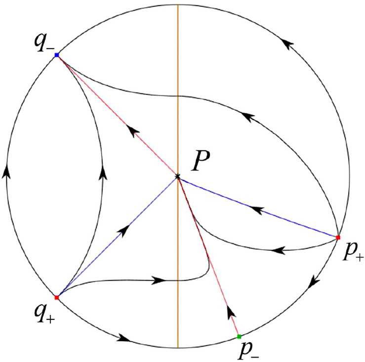
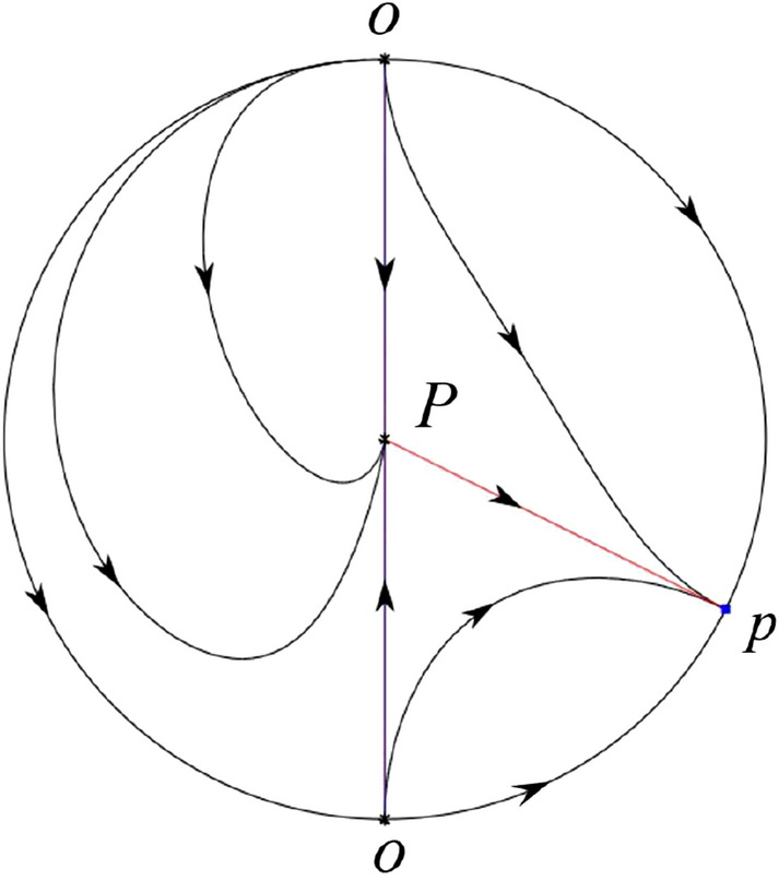
In the case (VI-1) one stable separatrix of the saddle-node P lying on the positive y-axis comes from the unstable node O in the positive y-direction, while the second stable separatrix of P lying on the negative y-axis comes from the unstable node O in the negative y-direction. The unstable separatrix of the saddle q goes to P. The unstable separatrix of P goes to the stable node p. The remaining orbits of the phase portrait are determined where they start and they end by the type of stability of the equilibrium points and by the Poincaré–Bendixson theorem. Thus the global phase portrait is shown in Fig. 60.
Fig. 60.
In the case (VI-2) one stable separatrix of P comes from the unstable node O in the positive y-direction and the second stable separatrix of P comes from the saddle-node O in the negative y-direction. An unstable separatrix of P goes to the stable node p. The remaining orbits of the phase portrait are determined by the type of stability of the equilibrium points and by the Poincaré–Bendixson theorem. Thus the global phase portrait is shown in Fig. 61.
Fig. 61.
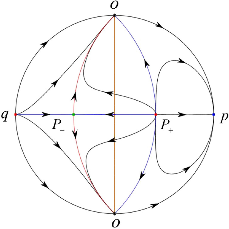
In the case (VI-3) one stable separatrix of P lying on the positive y-axis comes from the unstable node O in the positive y-direction of the half plane and the second stable separatrix of P lying on the negative y-axis comes from the unstable node O in the negative y-direction of the half plane . An unstable separatrix of the saddle P in the half plane goes to the stable node p. The infinity of is filled with equilibrium points. At each one of these equilibrium points starts an orbit going to the stable node P in the half plane . The remaining orbits of the phase portrait are determined by the type of stability of the equilibrium points and by the Poincaré–Bendixson theorem. Thus the global phase portrait is shown in Fig. 62.
Fig. 62.

In the case (VI-4) one stable separatrix of P comes from the saddle-node O in the positive y-direction and the second stable separatrix of P comes from the unstable node O in the negative y-direction. An unstable separatrix of P goes to the stable node p. The remaining orbits of the phase portrait are determined by the type of stability of the equilibrium points and by the Poincaré–Bendixson theorem. Thus the global phase portrait is shown in Fig. 63.
Fig. 63.
In the case (VI-5) one stable separatrix of P comes from the saddle-node O in the positive y-direction and the second stable separatrix of P comes from the saddle-node O in the negative y-direction. An unstable separatrix of P goes to the stable node p. The remaining orbits of the phase portrait are determined by the type of stability of the equilibrium points and by the Poincaré–Bendixson theorem. Thus the global phase portrait is shown in Fig. 64.
Fig. 64.
In the case (VI-6) one unstable separatrix of P goes to the saddle-node O in the positive y-direction and the second unstable separatrix of P goes to the saddle-node O in the negative y-direction. A stable separatrix of P comes from the unstable node q. The remaining orbits of the phase portrait are determined by the type of stability of the equilibrium points and by the Poincaré–Bendixson theorem. Thus the global phase portrait is shown in Fig. 65.
Fig. 65.
In the case (VI-7) one unstable separatrix of P goes to the saddle-node O in the positive y-direction and the second unstable separatrix of P goes to the stable node O in the negative y-direction. A stable separatrix of P comes from the unstable node q. On the other hand by the type of stability of the equilibrium points and by the Poincaré–Bendixson theorem we get the remaining orbits of the phase portrait. Thus the global phase portrait is shown in Fig. 66.
Fig. 66.
In the case (VI-8) one unstable separatrix of P goes to the stable node O in the positive y-direction of the half plane and the second unstable separatrix of P goes to the stable node O in the negative y-direction of the half plane . A stable separatrix of P comes from the unstable node q. The infinity of is filled with equilibrium points. At each one of these infinite equilibrium points arrives an orbit starting at the unstable node P in the half plane . By the type of stability of the equilibrium points and by the Poincaré–Bendixson theorem we get the remaining orbits of the phase portrait. Thus the global phase portrait is shown in Fig. 67.
Fig. 67.
In the case (VI-9) a stable separatrix of P comes from the unstable node q. One unstable separatrix of P goes to the stable node O in the positive y-direction. The second unstable separatrix of P goes to the saddle-node O in the negative y-direction. By the type of stability of the equilibrium points and by the Poincaré–Bendixson theorem we get the remaining orbits of the phase portrait. Thus the global phase portrait is shown in Fig. 68.
Fig. 68.

In the case (VI-10) a stable separatrix of P comes from the unstable node q in the half plane . One unstable separatrix of P lying on the positive y-axis goes to the stable node O and the second unstable separatrix of P lying on the negative y-axis goes to the stable node O in the half plane . The stable separatrix of the saddle p comes from P. We obtain the remaining orbits of the phase portraits by the type of stability of the equilibrium points and by the Poincaré–Bendixson theorem. Thus the global phase portrait is shown in Fig. 69.
Fig. 69.
The Distinct Topologically Equivalent Phase Portraits
In this section we summarize the results on the distinct topological equivalent phase portraits from Figs. 17 to 69.
By the separatrix configuration of the phase portrait in Theorem 2 we have the following XIX categories
- I.
- II.
- III.
- IV.
- V.
-
VI.
Figure 23;
- VII.
- VIII.
-
IX.
Figures 31, 33, 61, 63, 66 and 68 are topologically equivalent;
-
X.
Figure 32;
- XI.
-
XII.
Figures 36, 38, 51, 53, 56 and 58 are topologically equivalent;
-
XIII.
Figure 37;
- XIV.
- XV.
- XVI.
- XVII.
- XVIII.
- XIX.
This proves the first part of Theorem 1 and Fig. 1 comes from Figs. 17, 18, 19, 20, 21, 23, 28, 30, 31, 32, 35, 36, 37, 42, 44, 52, 54, 62, 64.
Fig. 22.
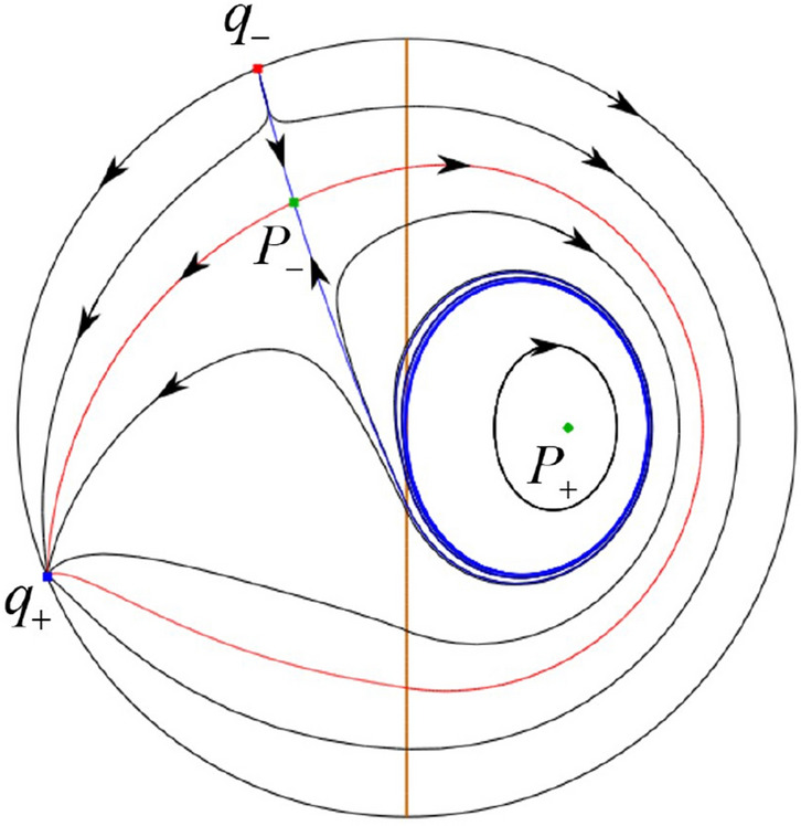
Fig. 24.
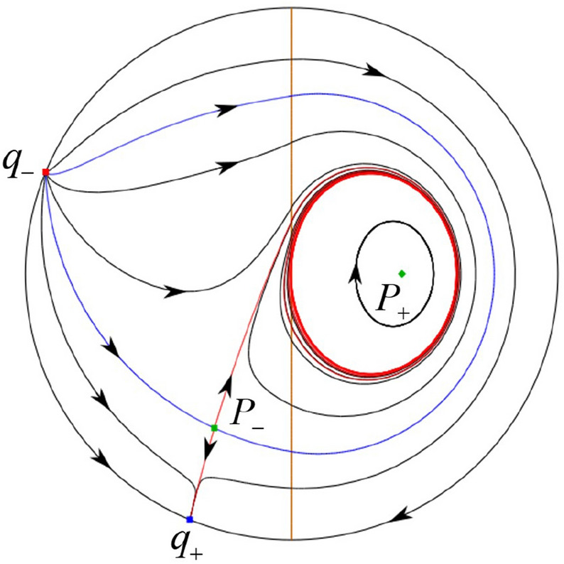
Fig. 23.
Funding
Open Access Funding provided by Universitat Autonoma de Barcelona. The first author is partially supported by natural science starting project of SWPU (No. 2023QHZ016).The second author is is partially supported by the Agencia Estatal de Investigación grant PID2019-104658GB-I00, the H2020 European Research Council grant MSCA-RISE-2017-777911, AGAUR (Generalitat de Catalunya) grant 2022-SGR 00113, and by the Acadèmia de Ciències i Arts de Barcelona.
Data availability
The data underlying this article are available.
Declarations
Conflict of interest
Authors do not have any conflicts of interest.
References
- 1.Andronov, A., Vitt, A., Khaikin, S.: Theory of Oscillations. Pergamon Press, Oxford (1966) [Google Scholar]
- 2.de Freitas, B.R., Llibre, J., Medrado, J.C.: Limit cycles of continuous and discontinuous piecewise-linear differential systems in R3. J. Comput. Appl. Math. 338, 311–323 (2018) [Google Scholar]
- 3.di Bernardo, M., Budd, C.J., Champneys, A.R., Kowalczyk, P.: Piecewise-Smooth Dynamical Systems: Theory and Applications. Applied Mathematical Sciences Series 163. Springer, London (2008) [Google Scholar]
- 4.Diz-Pita, E., Llibre, J., Otero-Espinar, M.V.: Phase portraits of a family of Kolmogorov systems with many singular points at infinity. Commun. Nonlinear Sci. Numer. Simul. 104, 106038–16 (2022) [Google Scholar]
- 5.Dumortier, F., Llibre, J., Artés, J.C.: Qualitative Theory of Planar Differential Systems. Springer, New York (2006) [Google Scholar]
- 6.Freire, E., Ponce, E., Rodrigo, F., Torres, F.: Bifurcation sets of continuous piecewise linear systems with two zones. Int. J. Bifurc. Chaos 8, 2073–2097 (1998) [Google Scholar]
- 7.Freire, E., Ponce, E., Torres, F.: Canonical discontinuous planar piecewise linear systems. SIAM J. Appl. Dyn. Syst. 119, 181–211 (2012) [Google Scholar]
- 8.Hirsch, M.W., Pugh, C.C., Shub, M.: Invariant Manifolds. Lecture Notes in Mathematics, vol. 583. Springer, Berlin (1977) [Google Scholar]
- 9.Li, S., Llibre, J.: Phase portraits of piecewise linear continuous differential systems with two zones separated by a straight line. J. Differ. Equ. 266, 8094–8109 (2019) [Google Scholar]
- 10.Li, S., Llibre, J.: Phase portraits of planar piecewise linear refracting systems: focus-saddle case. Nonlinear Anal. Real World Appl. 56, 103153 (2020) [Google Scholar]
- 11.Llibre, J., Ordóñez, M., Ponce, E.: On the existence and uniqueness of limit cycles in a planar piecewise linear systems without symmetry. Nonlinear Anal. Real World Appl. 14, 2002–2012 (2013) [Google Scholar]
-
12.Lum, R., Chua, L.O.: Global properties of continuous piecewise linear vector fields. Part I: simplest case in
 . Int. J. Circuit Theory Appl. 19, 251–307 (1991) [Google Scholar]
 -
13.Lum, R., Chua, L.O.: Global properties of continuous piecewise linear vector fields. Part II: simplest symmetric case in
 . Int. J. Circuit Theory Appl. 20, 9–46 (1992) [Google Scholar]
 - 14.Makarenkov, O., Lamb, J.S.W.: Dynamics and bifurcations of nonsmooth systems: a survey. Phys. D 241, 1826–1844 (2012) [Google Scholar]
- 15.Markus, L.: Global structure of ordinary differential equations in the plane. Trans. Am Math. Soc. 76, 127–148 (1954) [Google Scholar]
- 16.Neumann, D.A.: Classification of continuous flows on 2-manifolds. Proc. Am. Math. Soc. 48, 73–81 (1975) [Google Scholar]
- 17.Peixoto, M.M.: On the Classification of Flows on 2-Manifolds, pp. 389–419. Academic, New York (1973). Dynamical Systems (Proceedings of a Symposium University of Bahia, Salvador, 1971)
- 18.Simpson, D.J.W.: Bifurcations in Piecewise-Smooth Continuous Systems. World Scientific Series on Nonlinear Science Series A, vol. 69. World Scientific, Singapore (2010) [Google Scholar]
- 19.Zhang, Z., Ding, T., Huang, W., Dong, Z.: Qualitative Theory of Differential Equations. Amer. Math. Soc., Providence (1992) [Google Scholar]
Associated Data
This section collects any data citations, data availability statements, or supplementary materials included in this article.
Data Availability Statement
The data underlying this article are available.