Clinical, radiological, and radiomics feature-based explainable machine learning models for prediction of neurological deterioration and 90-day outcomes in mild intracerebral hemorrhage

Abstract

Background

The risks and prognosis of mild intracerebral hemorrhage (ICH) patients were easily overlooked by clinicians. Our goal was to use machine learning (ML) methods to predict mild ICH patients’ neurological deterioration (ND) and 90-day prognosis.

Methods

This prospective study recruited 257 patients with mild ICH for this study. After exclusions, 148 patients were included in the ND study and 144 patients in the 90-day prognosis study. We trained five ML models using filtered data, including clinical, traditional imaging, and radiomics indicators based on non-contrast computed tomography (NCCT). Additionally, we incorporated the Shapley Additive Explanation (SHAP) method to display key features and visualize the decision-making process of the model for each individual.

Results

A total of 21 (14.2%) mild ICH patients developed ND, and 35 (24.3%) mild ICH patients had a 90-day poor prognosis. In the validation set, the support vector machine (SVM) models achieved an AUC of 0.846 (95% confidence intervals (CI), 0.627-1.000) and an F1-score of 0.667 for predicting ND, and an AUC of 0.970 (95% CI, 0.928-1.000), and an F1-score of 0.846 for predicting 90-day prognosis. The SHAP analysis results indicated that several clinical features, the island sign, and the radiomics features of the hematoma were of significant value in predicting ND and 90-day prognosis.

Conclusion

The ML models, constructed using clinical, traditional imaging, and radiomics indicators, demonstrated good classification performance in predicting ND and 90-day prognosis in patients with mild ICH, and have the potential to serve as an effective tool in clinical practice.

Clinical trial number

Not applicable.

Supplementary Information

The online version contains supplementary material available at 10.1186/s12880-025-01717-x.

Introduction

Intracerebral hemorrhage (ICH) is the second most common subtype of stroke, often resulting in severe disability or death, making it a critical medical condition [1]. In clinical practice, physicians often pay more attention to comatose ICH patients who require surgical treatment. However, mild ICH, which refers to patients who are conscious and present with relatively mild symptoms that do not necessitate surgery, still poses specific challenges [2]. The treatment plan for ICH patients is generally determined by clinicians based on a subjective assessment of the patient’s symptoms and neurological function. Mild ICH patients, who exhibit milder early symptoms and are treated conservatively, typically have a better prognosis. However, they still face the risk of early hematoma expansion (HE) and neurological deterioration (ND), which are adverse events that often lead to poor outcomes [3].

Previous studies have conducted in-depth explorations of risk factors for poor prognosis in ICH. Clinical and imaging characteristics are considered important tools for prognostic assessment in ICH. For example, the prognosis of ICH is closely related to the baseline ICH volume and neurological function scores at admission [4]. Major risk factors for ND include advanced age, high NIHSS scores at admission, large baseline hematoma volume, and hematoma expansion [3]. HE and peak perihematomal edema (PHE) are independent predictors of poor functional outcomes and increased mortality in ICH patients [5, 6]. The factors influencing the prognosis of mild ICH patients are numerous and highly complex. Machine learning (ML) can accurately process complex nonlinear relationships among many of variables, a challenging task for traditional statistical models [7, 8]. This technology has been applied to assess the risk of ND and HE, as well as prognosis in ICH patients, and it is showing great promise in the field of ICH [9–11].

Similar to previous studies, in our extensive clinical practice, we have observed that clinicians often focus more on severe ICH patients who require surgical treatment. In contrast, for ICH patients with milder symptoms and clear consciousness who are treated conservatively with medication, neurologists may not actively follow up due to their relatively better prognosis. To avoid overtreatment and prevent overlooking deterioration risks, a clinically applicable system is needed to identify high-risk mild ICH patients for early focus and intervention. Therefore, we included mild ICH patients who did not undergo surgical treatment and grouped them based on ND during hospitalization and their 90-day modified Rankin Scale (mRS-90) scores. Through this study, we aim to explore the following questions: [1] whether the ML models based on clinical, imaging, and radiomics features can accurately predict the ND and mRS-90 of mild ICH patients, and [2] which risk factors for poor prognosis in severe ICH patients can be used for prognostic assessment in mild ICH patients.

Methods

Ethics statements

This prospective study has obtained approval from the Medical Ethics Committee of Nanfang Hospital (approval number: NFEC-2022-168). All participants provided written consent before participating in the study.

Study design and participants

This prospective study was conducted on 257 patients with mild ICH. Conscious ICH patients in the study who had relatively mild symptoms and did not require surgery were admitted from the neurology wards from November 2018 to December 2023 at Nanfang Hospital. Whether these patients developed ND and their mRS-90 scores were recorded. ND was defined as: [1] an increase of ≥ 4 points in the NIHSS score within 15 days of onset; [2] a decrease of ≥ 1 point in the Glasgow Coma Scale (GCS) within 15 days of onset. The mRS-90 score ≤ 2 was defined as good prognosis, while the mRS-90 score > 2 was defined as poor prognosis. As shown in Fig. 1, 148 patients were included for the ND study, and 144 patients were included for the 90-day prognosis study after exclusions. Notably, the mRS-90 dataset excluded an additional 4 cases lacking 90-day follow-up data compared to the ND dataset. The sample size was calculated based on a significant difference test for the incidence of adverse clinical outcome (α = 0.05, 1-β = 0.8, power = 0.8) via MedCalc 19.0.7 (MedCalc Software Ltd., Ostend, Belgium) and the details are shown in Supplementary Figs. 1–2. Calculations indicated that the sample size included in this study met the required total sample size for both the ND and mRS datasets. The inclusion criteria were as follows: [1] the ICH patients with mild symptoms and did not require surgery; [2] the National Institutes of Health Stroke Scale (NIHSS) < 15 and ICH score ≤ 2; [3] time from onset to admission ≤ 48 h; [4] at least one head CT scan performed within one week after onset. The exclusion criteria were as follows: [1] age > 80 years; [2] premorbid mRS score > 2; [3] the hematoma was located in the infratentorial region; [4] history of cerebral hemorrhage, subarachnoid hemorrhage, arterial or venous malformations, intracranial aneurysms or tumors; [5] imaging data was missing or the image quality was too poor to complete radiological analysis; [6] lost to follow-up after discharge, making it impossible to obtain the mRS-90 score; [7] comorbid hematological conditions, malignant tumors, severe heart and renal failure.

Fig. 1.

The schema of study workflow

This study adheres to the transparent reporting of a multivariable prediction model for individual prognosis or diagnosis (TRIPOD) guidelines, focusing on developing prediction models for ND and 90-day functional prognosis in patients with mild ICH [12]. Additionally, the Radiomics Quality Score (RQS) for this study is 72.22%, and METhodological RadiomICs Score (METRICS) is 77.7% [13, 14].

Medical records and clinical assessments

Baseline demographic and clinical characteristics were recorded. The mRS-90 indicated patients’ long-term functional outcome as primary endpoints. We divided the patients into two groups: mRS-90 ≤ 2 was defined as good prognosis, and mRS-90 > 2 was defined as poor prognosis. Similarly, patients were divided into two groups to assess short-term functional observation points based on the occurrence of ND as secondary endpoints. The ND was defined as an increase in NIHSS by ≥ 4 points or a decrease in Glasgow Coma Scale (GCS) by ≥ 1 point during hospitalization [15, 16]. A neurologist (W.Q., 15 years’ experience) reviewed the accuracy of the clinical data and checked for missing data and outliers. For the mRS-90 prediction task, we used the available clinical data from patient admission to discharge. For the ND prediction task, we used baseline clinical data at admission, excluding any changes in condition during hospitalization. Features with missing values exceeding 25% were excluded. Missing values in the remaining clinical features were imputed using random forest. Detailed details of the missing value imputation method can be found in Supplementary Material 1, and the missing data reports and pre-post imputation data comparisons are provided in Supplementary Tables 1–3.

Radiological assessment

All NCCT images were downloaded in digital imaging and communications in medicine (DICOM) format. The summary of NCCT imaging parameters in this study is shown in Supplementary Table 4. An experienced neuroimaging researcher (Z.W., 5 years’ experience), who was blinded to patients’ baseline demographic and clinical characteristics, assessed traditional imaging features of hematoma from baseline non-contrast computed tomography (NCCT) scans. The assessment content included three shape features (island sign [17], satellite sign [18], margin irregularity [19, 20]) and five density features (low density sign [19], swirl sign [21], black hole sign [22], blend sign [23], density heterogeneity [19, 20]). Margin irregularity and density heterogeneity were classified into five levels based on previous studies [19, 20]. Additionally, the evaluation included whether the ICH had broken into the ventricles and the presence of subarachnoid hemorrhage. Examples of each imaging sign are illustrated in Fig. 2, and detailed evaluation criteria according to reference are provided in Supplementary Material 2. Then, similarly, another experienced neuroimaging researcher (C.W., 40 years’ experience) reviewed and checked the evaluation of the traditional imaging features. Information such as the volume, density, and diameters of the hematoma and perilesional edema were obtained from the radiomics features. Observer consistency analyses were performed, with the detailed implementation described in Supplementary Material 3. Results of intra-observer consistency analysis showed ICC values of 0.887 (95% confidence intervals (CI), 0.742–0.950) for traditional imaging features. Results of inter-observer consistency analysis showed ICC values of 0.932 (95% CI 0.829–0.966). We had provided the ICC values for each specific feature in Supplementary Table 5.

Fig. 2.

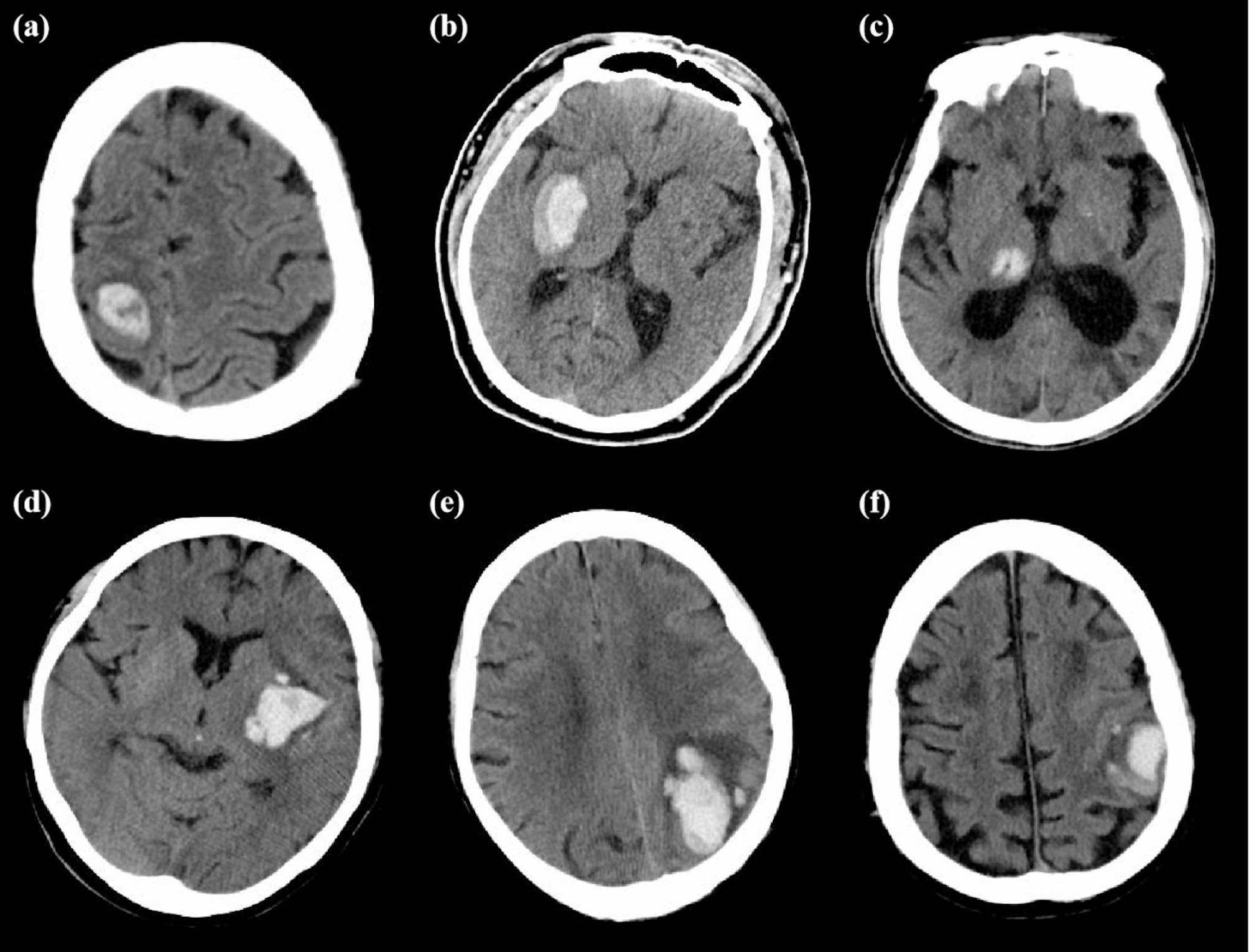
Examples of each imaging sign of traditional imaging features: (a) Swirl sign; (b) Blend sign; (c) Black hole sign; (d) Low density sign; (e) Island sign; (f) Satellite sign

Preprocessing of images and radiomics feature extraction

The images were uploaded to ITK-SNAP software (version 3.8.0) for the segmentation of the region of interest (ROI). We defined hematoma and perilesional edema as two separate ROIs. Each image provided separate 3D-ROIs performed by delineating along the lesion boundary layer by layer. An experienced neuroimaging researcher (Z.W., 5 years’ experience) performed the manual segmentation. Another experienced neuroimaging researcher (C.W., 40 years’ experience) checked the segmentation results. Observer consistency analyses were performed, with the detailed implementation described in Supplementary Material 3. Results of intra-observer consistency analysis showed ICC values of 0.980 (95% CI, 0.955–0.992) for hematoma and 0.767 (95% CI, 0.472–0.897) for perilesional edema. Results of inter-observer consistency analysis showed ICC values of 0.938 (95% CI, 0.855–0.973) for hematoma and 0.736 (95% CI, 0.402–0.884) for perilesional edema.

Prior to radiomics feature extraction, we performed image preprocessing, which included standardization and filtering. All steps were implemented in Python 3.7.4 (Python Software Foundation, Wilmington, DE, USA). Global normalization was applied to standardize all images. The workflow was as follows: images were converted to Numpy arrays using the SimpleITK (v2.2.0) library, followed by calculation of the global mean intensity () and variance (). The normalization formula was then applied, and normalized arrays were converted back to SimpleITK image format. Filtering was performed using the Pyradiomics (version 3.0.1) library [24] during feature extraction process, including Original (no processing), Wavelet, LoG, Square, SquareRoot, Logarithm, Exponential, Gradient, LBP2D, and LBP3D. The types of extracted radiomic features included shape features, first order features, textural features, wavelet features, and other transformed features. A total of 1691 radiomics features were extracted from ROI of hematoma and perilesional edema.

Then, we further selected radiomics features of hematoma via the following two steps: [1] features with a Spearman correlation coefficient ≥ 0.8 were selected; [2] using the LASSO regression to determine the final radiomics features strongly correlated with the prediction target. Then, the radiomics score (Rad-score) for each patient was calculated as a weighted linear combination of the selected features’ non-zero coefficients. Feature selection was performed separately for the mRS-90 and ND tasks, resulting in two different sets of selected radiomics features. The implementation details of LASSO regression for radiomics feature selection can be found in Supplementary Material 4. Given the relatively low density heterogeneity of edema surrounding the hematoma and to improve interpretability, this study exclusively incorporated shape and first-order features of perilesional edema strongly correlated with the aforementioned metrics.

Model development and evaluation

Two datasets were constructed, which included baseline demographic, and clinical characteristics, radiomics features and traditional imaging features of baseline NCCT scans. The dataset was randomly divided into a training set and a validation set at a ratio of 7:3. Using the MinMaxScaler module from the scikit-learn library, we normalized quantitative features to the range of 0–1. First, the training set was normalized by calculating the minimum and maximum values for each feature and mapping the training data to the [0, 1] interval. Subsequently, the validation set was transformed using the same min-max parameters derived from the training set to complete standardization while avoiding data leakage. These procedures were independently performed on both the mRS-90 and the ND datasets, respectively. To address the issue of unbalanced sample sizes in patients with poor prognosis and ND, we employed the synthetic minority oversampling technique (SMOTE) to balance the training set for both classification tasks [25]. It is important to note that this step only processes features from the training set for subsequent machine learning model training, and the validation set used to evaluate the trained model still consists of real data. We employed two methods for feature selection in the training set: Logistics Regression with L1 regularization and Recursive Feature Elimination (RFE). The implementation details of Logistics Regression for feature selection can be found in Supplementary Material 5. Following the above process, the mRS-90 and ND prediction task feature sets were constructed separately.

In this study, we developed and validated five ML algorithms, including Support Vector Machine (SVM) [26], Random Forest Classifier (RFC) [27], Extreme Gradient Boosting (XGBoost) [28], Gradient Boosting Machine (GBM) [29], and k-Nearest Neighbors (KNN) [30]. These models were implemented using the scikit-learn and XGBoost packages. Model derivation and internal validation were conducted using ten-fold cross-validation. The grid search method was employed during the training process to optimize the models’ hyperparameters. Ten-fold cross-validation is a method that divides a dataset into 10 subsamples, trains a model on 9 subsamples and validates it on 1 subsample, repeats this process 10 times, and uses the average performance as the evaluation result [31]. The specific parameter details of each model in the two prediction tasks are presented in Supplementary Tables 6–7. The AUC, sensitivity, specificity, accuracy, and F1-score of the ML models were calculated in the validation set to assess the classification performance. Decision curve analysis (DCA) was used to evaluate the models’ clinical usefulness and net benefit. Shapley Additive Explanations (SHAP) local interpretation technique was used to evaluate the interpretability of the optimal model. This method explains the optimal model by calculating the contribution of each feature to the prediction results individually and globally [32, 33]. Through SHAP’s global interpretation methods, we could generate bar plots and beeswarm plots to observe the global feature importance of the models in each prediction task. Through SHAP’s local interpretation methods, we can generate force plots to display the models’ decision-making process for individual cases. The schema of the study workflow is shown in Fig. 1.

Statistical analysis

The statistical analysis in this study was conducted using RStudio 4.0.3 (R Foundation for Statistical Computing, Vienna, Austria). Univariate analyses were performed using the independent sample t-test and Mann-Whiney U test. The independent sample t-test assumed that the continuous variables in each group followed a normal distribution and had homogeneity of variances. These assumptions were verified using the Shapiro-Wilk test for normality for variance homogeneity. When these assumptions were violated, the non-parametric Mann-Whitney U test, which only requires independent observations, was used instead. Chi-square test and Fisher’s exact test were used to analyze categorical data. The chi-square test assumed that the observations were independent and the expected frequencies in each cell of the contingency table were at least 5. When the expected frequencies were small (less than 5), Fisher’s exact test, which also assumes independent observations, was applied. The AUCs of ML models, Rad_score, and admission mRS (mRS-ad) were compared using the DeLong test in MedCalc 19.0.7 (MedCalc Software Ltd., Ostend, Belgium). The DeLong test assumes that the models are evaluated on the same set of subjects (paired observations) and that the predictions of different models are dependent.

Results

Study population

Descriptive statistics and intergroup comparative analyses of ND and mRS-90 are shown in Tables 1 and 2. These analyses were considered descriptive and were not adjusted for other covariates. A total of 148 patients were included for predicting ND (n = 21, 14.2%), and 144 patients were included for predicting mRS-90 (n = 35, 24.3%). The complete content of the intergroup comparison analysis is presented in Supplementary Tables 8–9.

Table 1.

Summary of the baseline clinical, imaging, and radiomics characteristics comparing mild ICH patients with ND

	Non-ND	ND	Total	p
	(N = 127)	(N = 21)	(N = 148)
Age	56.97 ± 11.35	59.24 ± 14.47	57.29 ± 11.82	0.417
BMI	24.52 ± 3.32	24.01 ± 3.59	24.44 ± 3.35	0.526
Female	36 (28.35%)	4 (19.05%)	40 (27.03%)	0.533
Admission NIHSS	5.00 [2.00;8.00]	9.00 [7.00;12.00]	6.00 [2.00;9.00]	< 0.001*
Admission GCS	15.00 [14.50;15.00]	14.00 [13.00;15.00]	15.00 [14.00;15.00]	< 0.001*
Admission systolic blood pressure	149.00 [139.00;160.00]	166.00 [139.00;179.00]	150.00 [139.00;162.50]	0.041*
Admission diastolic blood pressure	88.83 ± 13.32	88.67 ± 13.29	88.80 ± 13.27	0.959
ICH score				0.051
0	83 (65.35%)	9 (42.86%)	92 (62.16%)
1	39 (30.71%)	9 (42.86%)	48 (32.43%)
2	5 (3.94%)	3 (14.29%)	8 (5.41%)
Low density sign	50 (39.37%)	12 (57.14%)	62 (41.89%)	0.197
Black hole sign	11 (8.66%)	1 (4.76%)	12 (8.11%)	1.000
Swirl sign	15 (11.81%)	7 (33.33%)	22 (14.86%)	0.018*
Blend sign	12 (9.45%)	1 (4.76%)	13 (8.78%)	0.694
Island sign	35 (27.56%)	7 (33.33%)	42 (28.38%)	0.778
Satellite sign	14 (11.02%)	5 (23.81%)	19 (12.84%)	0.150
Intraventricular hemorrhage	13 (10.24%)	6 (28.57%)	19 (12.84%)	0.032*
Subarachnoid hemorrhage	0 (0.0%)	3 (14.29%)	3 (2.03%)	0.003*
Rad-score	0.00 [0.00;0.01]	0.00 [0.00;0.02]	0.00 [0.00;0.02]	0.055

Abbreviations: BMI, Body Mass Index; NIHSS, National Institutes of Health Stroke Scale; GCS, Glasgow Coma Scale; ICH, Intracerebral Hemorrhage; Rad-score, Radiomics Score

* Indicates p value < 0.05

Table 2.

Summary of the baseline clinical, imaging, and radiomics characteristics comparing mild ICH patients with poor prognosis

	mRS-90 ≤ 2	mRS-90 > 2	Total	p
	(N = 109)	(N = 35)	(N = 144)
Age	57.72 ± 11.92	56.66 ± 12.09	57.47 ± 11.93	0.647
BMI	24.17 ± 3.02	25.20 ± 4.32	24.42 ± 3.39	0.202
Female	31 (28.44%)	7 (20.00%)	38 (26.39%)	0.444
Admission NIHSS	4.00 [2.00;7.00]	11.00 [8.00;12.00]	6.00 [2.00;9.00]	< 0.001*
Admission GCS	15.00 [15.00;15.00]	14.00 [13.00;15.00]	15.00 [14.00;15.00]	< 0.001*
Admission systolic blood pressure	147.00 [136.00;160.00]	155.00 [144.50;169.50]	149.50 [139.00;162.50]	0.008*
Admission diastolic blood pressure	86.96 ± 12.31	94.09 ± 15.13	88.69 ± 13.35	0.006*
ICH score				< 0.001*
0	78 (71.56%)	12 (34.29%)	90 (62.50%)
1	27 (24.77%)	20 (57.14%)	47 (32.64%)
2	4 (3.67%)	3 (8.57%)	7 (4.86%)
Low density sign	42 (38.53%)	18 (51.43%)	60 (41.67%)	0.250
Black hole sign	9 (8.26%)	3 (8.57%)	12 (8.33%)	1.000
Swirl sign	15 (13.76%)	5 (14.29%)	20 (13.89%)	1.000
Blend sign	11 (10.09%)	2 (5.71%)	13 (9.03%)	0.735
Island sign	20 (18.35%)	18 (51.43%)	38 (26.39%)	< 0.001*
Satellite sign	7 (6.42%)	11 (31.43%)	18 (12.50%)	< 0.001*
Intraventricular hemorrhage	10 (9.17%)	9 (25.71%)	19 (13.19%)	0.020*
Subarachnoid hemorrhage	0 (0.0%)	3 (8.57%)	3 (2.08%)	0.013*
Rad-score	57843.65 [18263.46;105265.20]	128061.46 [60880.95;248681.41]	63278.88 [20392.31;136697.96]	< 0.001*

Abbreviations: BMI, Body Mass Index; NIHSS, National Institutes of Health Stroke Scale; GCS, Glasgow Coma Scale; ICH, Intracerebral Hemorrhage; Rad-score, Radiomics Score

* Indicates p value < 0.05

Dataset comparison

We compared the features in the ND dataset and mRS-90 dataset before and after random forest imputation (Supplementary Tables 2–3). Results showed no statistical differences for all features before imputation (p > 0.05).

Additionally, we conducted intergroup comparisons for the training and validation sets randomly split in the ND dataset and mRS-90 dataset, respectively. The results are shown in Supplementary Tables 10–11. In the ND dataset, only rad_score and TP showed significant differences between the training and validation sets (p = 0.024; p = 0.005), while no significant differences were observed for other features (p > 0.05). In the mRS-90 dataset, all features exhibited no significant differences between the training and validation sets (p > 0.05).

Feature selection and dimensionality reduction

We performed feature dimensionality reduction on the radiomics features extracted from the hematoma ROI using Spearman correlation coefficient and LASSO regression. Subsequently, we combined the baseline demographic and clinical characteristics, imaging signs, hematoma-based radiomics features after Spearman correlation analysis and LASSO regression dimensionality reduction, and shape and first-order features based on perilesional edema into a feature set. Finally, we further completed feature selection on this combined feature set through Logistic Regression with L1 regularization and RFE, obtaining the feature set required by the model. As shown in Fig. 3, the LASSO regression analysis process filtered out less-relevant features by gradually shrinking coefficients as λ increases and considered the MSE to determine the optimal parameter. Then, a total of 4 hematoma radiomics features were selected in the ND dataset, while a total of 5 hematoma radiomics features were selected in the mRS-90 dataset. Finally, through feature selection using Logistic Regression and RFE, a total of 28 features were selected in the ND dataset, and 28 features were selected in the mRS-90 dataset.

Fig. 3.

LASSO regression analysis results. (a, b) Feature coefficient path diagram and mean squared error curve of the ND dataset; (c, d) Feature coefficient path diagram and mean squared error curve of the mRS-90 dataset

Model performance

Two sets of ML models were constructed to predict poor prognosis (mRS-90 > 2) and ND of patients with mild ICH.

Task of predicting ND

Using random stratified sampling, the dataset was divided into a training set (n = 103, 69.6%) and a validation set (n = 45, 30.4%). There were 15 patients with poor prognosis in the training set, and 6 patients with poor prognosis in the validation set. As shown in Fig. 4; Table 3, in the validation set, the ML models (SVM, RF, XGB, GBM, KNN) predicting mRS-90 had AUCs of 0.846 (95% CI, 0.627-1.000), 0.861 (95%CI, 0.732–0.990), 0.850 (95%CI, 0.653-1.000), 0.829 (95%CI, 0.616-1.000), 0.806 (95%CI, 0.613–0.998), respectively. The DeLong test results indicate that there are no statistically significant differences in the AUC values among the five models based on clinical, imaging, and radiomics features and rad_score (Table 4). The model performance on the training set is shown in Supplementary Table 12. Decision curve analysis (DCA) showed that the net benefit obtained by the SVM model was significantly better than the other four ML models when the risk threshold probability was below 50%. Considering the adverse effects of underestimating patients’ risk, we selected the SVM model with higher precision and F1-score as the optimal prediction model for ND.

Fig. 4.

Classification of the five ML models for predicting ND. (a) The ROC of five ML models in the validation set. (b) The DCA of five ML models in the validation set

Table 3.

Classification performance of ML models for predicting ND in validation set

Model	AUC	Sensitivity	Specificity	Accuracy	F1-score	Youden
GBM	0.829 (0.616, 1.000)	0.500 (0.118, 0.882)	0.923 (0.791, 0.984)	0.867 (0.732, 0.950)	0.500	0.423
KNN	0.806 (0.613, 0.998)	0.500 (0.118, 0.882)	0.897 (0.758, 0.971)	0.844 (0.705, 0.935)	0.462	0.397
RF	0.861 (0.732, 0.990)	0.333 (0.043, 0.777)	0.949 (0.827, 0.994)	0.867 (0.732, 0.950)	0.400	0.282
XGB	0.850 (0.653, 1.000)	0.500 (0.118, 0.882)	0.949 (0.827, 0.994)	0.889 (0.760, 0.963)	0.546	0.449
SVM	0.846 (0.627, 1.000)	0.833 (0.359, 0.996)	0.897 (0.758, 0.971)	0.889 (0.760, 0.963)	0.667	0.731
Rad_score	0.658 (0.378, 0.893)	0.667 (0.200, 1.000)	0.769 (0.639, 0.897)	0.756 (0.622, 0.867)	0.421	0.436

Abbreviations: GBM, Gradient Boosting Machine; KNN, K-Nearest Neighbors; RF, Random Forest; XGB, Extreme Gradient Boosting; SVM, Support Vector Machine; AUC, area under the curve

Table 4.

Results of DeLong test between machine learning models and Rad_score for ND prediction in the validation set

	GBM	KNN	RF	SVM	XGB
KNN	0.686
RF	0.605	0.416
SVM	0.705	0.452	0.854
XGB	0.333	0.389	0.851	0.917
Rad_score	0.170	0.149	0.069	0.103	0.083

Abbreviations: GBM, Gradient Boosting Machine; KNN, K-Nearest Neighbors; RF, Random Forest; XGB, Extreme Gradient Boosting; SVM, Support Vector Machine; Rad-score, Radiomics Score; AUC, area under the curve

According to SHAP analysis (Fig. 5), the top five predictors in SVM model for predicting ND were 24-hour FOUR score, UA, “hematoma-gradient_ngtdm_Coarseness”, Acute Physiology and Chronic Health Evaluation II (APACHE-II) score, “hematoma-original_shape_LeastAxisLength”. In the CT images of the hematoma, “gradient_ngtdm_Coarseness” reflects the smoothness or irregularity of the hematoma edges, while “original_shape_LeastAxisLength” represents the shortest principal axis length of the hematoma in three-dimensional space.

Fig. 5.

The key features of the optimal model for predicting ND identified using the SHAP algorithm. (a) The global bar plot of SHAP values, with features ordered by their contribution to the ML model in descending order. (b) The beeswarm summary plot of SHAP values, illustrating the impact of these features on predictions

Task of predicting mRS-90

Using random stratified sampling, the dataset was divided into a training set (n = 100, 69.4%) and a validation set (n = 44, 30.6%) using random stratified sampling. There were 24 patients with poor prognosis in the training set, and 11 patients with poor prognosis in the validation set. As shown in Fig. 6; Table 5, the ML models (SVM, RF, XGB, GBM, KNN) predicting mRS-90 had AUCs of 0.970 (95%CI, 0.928-1.000), 0.959 (95%CI, 0.907-1.000), 0.960 (95%CI, 0.910-1.000), 0.926 (95%CI, 0.846-1.000), 0.796 (95%CI, 0.639–0.956), respectively. As shown in Table 6, DeLong test results showed the SVM model was significantly better than the KNN model (p = 0.025), and RF, SVM, XGB were significantly better than the Rad_score and mRS-ad (p < 0.05). The model performance on the training set are shown in Supplementary Table 13. DCA showed that the net benefit obtained by the SVM model was obviously better than that of the GBM and KNN models and slightly better than that of the XGB and RF models within the 35-45% range of risk threshold probability. Therefore, the SVM model was chosen as the optimal prediction model for poor prognosis in patients with mild ICH.

Fig. 6.

Classification of the five ML models for predicting poor prognosis. (a) The ROC of five ML models in the validation set. (b) The DCA of five ML models in the validation set

Table 5.

Classification performance of ML models for predicting mRS-90 in validation set

Model	AUC	Sensitivity	Specificity	Accuracy	F1-score	Youden
GBM	0.926 (0.846, 1.000)	0.636 (0.308, 0.891)	0.909 (0.757, 0.981)	0.841 (0.699, 0.934)	0.667	0.546
KNN	0.796 (0.636, 0.956)	0.455 (0.168, 0.766)	0.909 (0.757, 0.981)	0.796 (0.647, 0.902)	0.526	0.364
RF	0.959 (0.907, 1.000)	0.546 (0.234, 0.833)	1.000 (0.894, 1.000)	0.886 (0.754, 0.962)	0.706	0.546
XGB	0.960 (0.910, 1.000)	0.636 (0.308, 0.891)	0.970 (0.842, 0.999)	0.886 (0.754, 0.962)	0.737	0.606
SVM	0.970 (0.928, 1.000)	1.000 (0.715, 1.000)	0.879 0.718, 0.966)	0.909 (0.783, 0.975)	0.846	0.879
Rad_score	0.749 (0.576, 0.918)	0.727 (0.444, 1.000)	0.758 (0.606, 0.886)	0.750 (0.614, 0.864)	0.593	0.485
mRS-ad	0.742 (0.611, 0.861)	1.000 (1.000, 1.000)	0.606 (0.438, 0.778)	0.705 (0.568, 0.841)	0.629	0.606

Abbreviations: GBM, Gradient Boosting Machine; KNN, K-Nearest Neighbors; RF, Random Forest; XGB, Extreme Gradient Boosting; SVM, Support Vector Machine; Rad-score, Radiomics Score; AUC, mRS-ad, admission modified Rankin Scale; AUC, area under the curve

Table 6.

Results of DeLong test between machine learning models for mRS-90 prediction in the validation set

	GBM	KNN	RF	SVM	XGB	Rad_score
KNN	0.156
RF	0.301	0.036*
SVM	0.279	0.025*	0.684
XGB	0.314	0.039*	0.937	0.734
Rad_score	0.054	0.414	0.011*	0.009*	0.008*
mRS-ad	0.008	0.573	< 0.001*	< 0.001*	< 0.001*	0.951

Abbreviations: GBM, Gradient Boosting Machine; KNN, K-Nearest Neighbors; RF, Random Forest; XGB, Extreme Gradient Boosting; SVM, Support Vector Machine; Rad-score, Radiomics Score; mRS-ad, admission modified Rankin Scale; AUC, area under the curve

* Indicates p value < 0.05

According to SHAP analysis (Fig. 7), the top five predictors in SVM model for predicting mRS-90 were NIHSS at admission, island sign, time from onset to admission, results of the WADA water swallowing test at admission, and hyperlipidemia.

Fig. 7.

The key features of the optimal model for predicting poor prognosis identified using the SHAP algorithm. (a) The global bar plot of SHAP values, with features ordered by their contribution to the ML model in descending order. (b) The beeswarm summary plot of SHAP values, illustrating the impact of these features on predictions. The colors represent feature values, ranging from high (red) to low (blue), and the horizontal position indicates whether the feature value contributes to a positive or negative prediction

Discussion

We developed a series of ML models to predict the 90-day prognosis and ND in patients with mild ICH. Our ML model leverages both clinical, traditional imaging, and radiomics indicators. These models are highly needed tools for risk prognosis assessment in clinical practice for patients with mild ICH. It has the potential to enable clinicians to identify patients with mild ICH who may experience deterioration, assess the development of secondary brain injury, and provide personalized treatment, such as implementing more aggressive interventions early for targeted patients.

Most studies indicated that ML could serve as an early clinical evaluation tool to predict ND, PHE, and 90-day functional outcomes in patients with ICH [9–11]. Several studies have constructed predictive models using radiomics information and traditional imaging features extracted from hematoma, achieving favorable performance [9, 34]. However, a subset of patients who are conscious and present with mild symptoms upon admission has not received adequate attention. These patients still have the potential to experience clinical deterioration or poor outcomes during the course of their illness, and their risk factors are still being explored [2, 35, 36]. ND after ICH is not uncommon and is defined as an increase in NIHSS score by ≥ 4 points or a decrease in GCS score by ≥ 1 points, occurring in about 20% of ICH patients [15, 16]. The primary objective of this study was to develop ML models integrating information from multiple sources to predict the risk of ND and 90-day adverse outcomes in patients with mild ICH. The results demonstrated that ML also exhibited good predictive performance in this aspect. Several machine learning models significantly outperformed mRS-ad as a currently used clinical gold standard when predicting mRS-90 (p < 0.05). Considering the risk of underestimating the adverse events in patients, we selected SVM as the optimal model for predicting mRS-90 and ND after comprehensively evaluating AUC, F1-score, sensitivity, and other indicators.

The model results indicated that admission NIHSS, island sign, the WADA water swallowing test, time from onset to admission, and hyperlipidemia were the top five predictors of 90-day functional outcomes. The ND prediction model results indicate that 24-hour FOUR score, UA, APACHE-II score, “hematoma-gradient_ngtdm_Coarseness”, and “hematoma-original_shape_LeastAxisLength” were the top five predictors. However, despite these predictors having the highest importance weights in the model, it must be emphasized that they alone were insufficient to predict mRS-90 and ND reliably. The combined effect of all features contributed to this outcome.

Imaging markers of hematoma for poor prognosis included three shape features and five density features, which were discussed in this study. Among these, island sign, satellite sign, hematoma morphology classification, and hematoma density classification showed significant differences between poor and good prognosis groups (p < 0.05). Additionally, swirl sign and hematoma density classification showed significant differences between the ND and non-ND groups (p < 0.05). The model identified the island sign as a strong predictor of mRS-90. It was an imaging marker associated with PHE and poorer prognosis, and its formation may be due to the expansion of the hematoma causing rupture of adjacent small arteries, leading to focal or multifocal active bleeding [17].

Radiomics is an emerging high-throughput image analysis method. It involves extracting quantitative features from images to interpret lesions’ morphological characteristics and heterogeneity, aiding ML models in assessing hematoma risk [34, 37]. A strength of this study is the use of radiomics information from both the hematoma and the perilesional edema. The hematoma and perilesional edema were independently segmented as ROIs, and their radiomics features were extracted separately to be used for the model prediction tasks. In this study, some first-order radiomic features and texture features of the hematoma and perilesional edema were identified as important by the SVM model. The radiomics score of the hematoma showed a statistically significant difference between the poor prognosis group and the good prognosis group (p < 0.001). Among the radiomics features, “hematoma-original_shape_Maximum2DDiameterSlice” measures the largest diameter of the hematoma in a single CT slice, reflecting size, while “Hematoma-original_firstorder_Skewness” indicates asymmetry in intensity distribution, representing complexity. SHAP values suggest that for hematomas under 30 ml, lower values of these indicators predict a better prognosis. Previous studies found no significant correlation between hematoma volume and mRS-90 in mild ICH [35]. Coarseness reflects edge irregularity, with higher values indicating atypical growth [38]. The “LeastAxisLength” measures the shortest principal axis of the hematoma, and higher values may be associated with ND. Lastly, “edema-original_shape_Elongation” measures the shape of the perilesional edema. A higher elongation indicates a more stretched shape, which could be associated with more extensive brain injury. In addition, clinical and pathological evidence has shown that morphological characteristics of perilesional edema, including volume, surface area, growth pattern, and peak distance of expansion, are closely associated with functional outcomes in patients with ICH [39–41]. These features directly reflect edema’s spatial distribution and structural properties, which are critical for assessing edema progression and its mass effect on surrounding brain tissues. Given the relatively low density heterogeneity of perilesional edema and to improve interpretability, this study exclusively incorporated shape and first-order features strongly correlated with the aforementioned metrics. Through the force plot, we illustrated the detailed decision-making process of the model on an individual patient (Fig. 8). This method of local interpretation can help users more easily understand the operation and decision-making process of ML models, enabling doctors to intervene in patients’ personalized risk factors timely.

Fig. 8.

Two mild ICH cases were selected from the validation sets of the ND and mRS-90 prediction tasks, respectively. The decision-making process of the SVM model is illustrated using force plots. (a, c) Case #1, a 69-year-old male, experienced a hemorrhage in the left thalamus and subsequently developed ND during hospitalization. Despite a relatively low ICH score, due to factors including a low 24-hour FOUR score, high APACHE-II score, and other variables, the SVM model predicted that the patient had a high risk of ND. (b, d) Case #2, a 52-year-old male, experienced a hemorrhage in the right basal ganglia and temporal lobe and mRS-90 of 4. Due to factors including high NIHSS score at admission, high BMI, and the presence of the island sign, the SVM model predicted that this patient had a higher risk of poor 90-day prognosis. Each feature provides a SHAP value to the model’s base value. The final prediction value, f(x), is derived by the weighted sum of these features as processed by the model. When f(x) > 0, the model determines the condition to be ND or mRS > 2; otherwise, it is considered non-ND or mRS ≤ 2

In summary, this study constructed ML models to predict the risk of mRS-90 and ND in patients with mild ICH. Some risk factors previously used in studies to evaluate the prognosis of severe ICH patients can also be applied to machine learning models to predict the risk of ND and prognosis in mild ICH patients. Among them, the island sign was identified as a potential high-risk factor for poor prognosis in mild ICH. The radiomics features of the hematoma and perilesional edema were found to aid the ML models in making accurate predictions. Finally, this study employed SHAP-based model interpretation methods to visualize the feature importance and individualized risk factors for each patient. Mild ICH patients with potential risks of poor prognosis and ND may benefit from early intervention measures. Therefore, our predictive models could be practical and have additive value in clinical settings.

This study has some limitations. Firstly, due to the strict inclusion criteria, the sample size was relatively small. More samples and external validation are needed to evaluate the robustness and generalizability of the constructed models. Secondly, this study included patients with mild ICH who were conscious upon admission and had not undergone surgical treatment. Some mild ICH patients may undergo surgical treatment for other reasons, which may lead to selection bias in this study. Thirdly, the edges of the perilesional edema were blurred or too small in a few cases, making it difficult to delineate their ROI accurately.

Conclusion

This study focused on the short-term and long-term prognosis of patients with mild ICH and explored the value of clinical, traditional imaging, and radiomics indicators in predicting poor outcomes in these patients. The ML models constructed based on the above indicators demonstrated excellent classification performance in predicting mRS-90 and ND in patients with mild ICH. Combined with ML interpretability methods, the results of this study can provide an effective tool for early risk assessment and management of mild ICH patients in clinical practice.

Electronic supplementary material

Below is the link to the electronic supplementary material.

Abbreviations

APACHE-II

Acute Physiology and Chronic Health Evaluation II

ALT

Alanine aminotransferase ratio

AST

Aspartate aminotransferase

AUC

Area under curve

DCA

Decision curve analysis

FOUR

Fulloutline of Unresponsiveness Scale

GBM

Gradient Boosting Machine

GCS

Glasgow Coma Scale

HE

Hematoma expansion

hsTNT

High-sensitivity troponin T

ICH

Intracerebral hemorrhage

KNN

k-Nearest Neighbors

LYM%

Lymphocyte percentage

METRICS

METhodological RadiomICs Score

ML

Machine learning

mRS-90

90-day modified Rankin Scale

mRS-ad

Admission modified Rankin Scale

ND

Neurological deterioration

NCCT

Non-contrast computed tomography

NIHSS

National Institutes of Health Stroke Scale

PHE

Peak perihematomal edema

RQS

Radiomics Quality Score

RFC

Random Forest Classifier

Rad-score

Radiomics score

ROI

Region of interest

ROC

Receiver operating characteristic

SHAP

Shapley Additive Explanation

SVM

Support Vector Machine

XGBoost

Extreme Gradient Boosting

Author contributions

WZ: Conceptualization, Data curation, Formal analysis, Methodology, Visualization, Writing – original draft, Writing – review and editing. JC: Data curation, Writing – original draft, Writing – review and editing.LS: Data curation, Formal analysis, Methodology, Writing – original draft.GX: Data curation, Writing – review and editing.JX: Data curation, Writing – review and editing.SZ: Data curation, Formal analysis, Writing – review and editing.ZH: Methodology, Writing – review and editing.LD: Data curation, Formal analysis, Writing – review and editing.YG: Data curation, Writing – review and editing.JJY: Writing – review and editing.YL: Writing – review and editing.GQ: Methodology, Writing – review and editing.WC: Funding acquisition, Project administration, Supervision, Writing – review and editing.JY: Conceptualization, Funding acquisition, Project administration, Supervision, Writing – review and editing.QW: Conceptualization, Formal analysis, Funding acquisition, Methodology, Project administration, Supervision, Writing – review and editing.

Funding

This work was supported by National Natural Science Foundation of China [grant number 82171317], National Natural Science Foundation of China [grant number 82171929], National Natural Science Foundation of Guangdong Province [grant number 2022A1515010477], and President Foundation of Nanfang Hospital, Southern Medical University [grant number 2023A007].

Data availability

The data sets generated and/or analyzed by the current study can be obtained from the corresponding author upon reasonable request.

Declarations

Ethical approval

This prospective study has obtained approval from the Medical Ethics Committee of Nanfang Hospital (approval number: NFEC-2022-168). All study protocols and procedures were conducted in accordance with the Declaration of Helsinki.

Consent for publication

Not applicable.

Informed consent

All participants provided written consent before participating in the study.

Competing interests

The authors declare no competing interests.

References

- 1.An SJ, Kim TJ, Yoon BW, Epidemiology. Risk factors, and clinical features of intracerebral hemorrhage: an update. J Stroke. 2017;19:3–10. [DOI] [PMC free article] [PubMed]
- 2.Xu TQ, Lin WZ, Feng YL, et al. Leukoaraiosis is associated with clinical symptom severity, poor neurological function prognosis and stroke recurrence in mild intracerebral hemorrhage: a prospective multi-center cohort study. Neural Regen Res. 2022;17:819–23. [DOI] [PMC free article] [PubMed] [Google Scholar]
- 3.You S, Zheng D, Delcourt C, et al. Determinants of early versus delayed neurological deterioration in intracerebral hemorrhage. Stroke. 2019;50:1409–14. [DOI] [PubMed] [Google Scholar]
- 4.Morotti A, Boulouis G, Nawabi J, et al. Association between hematoma expansion severity and outcome and its interaction with baseline intracerebral hemorrhage volume. Neurology. 2023;101:e1606–13. [DOI] [PMC free article] [PubMed] [Google Scholar]
- 5.Davis SM, Broderick J, Hennerici M, et al. Hematoma growth is a determinant of mortality and poor outcome after intracerebral hemorrhage. Neurology. 2006;66:1175–81. [DOI] [PubMed] [Google Scholar]
- 6.Volbers B, Giede-Jeppe A, Gerner ST, et al. Peak perihemorrhagic edema correlates with functional outcome in intracerebral hemorrhage. Neurology. 2018;90:e1005–12. [DOI] [PubMed] [Google Scholar]
- 7.Deo RC. Machine learning in medicine. Circulation. 2015;132:1920–30. [DOI] [PMC free article] [PubMed] [Google Scholar]
- 8.Choy G, Khalilzadeh O, Michalski M, et al. Current applications and future impact of machine learning in radiology. Radiology. 2018;288:318–28. [DOI] [PMC free article] [PubMed] [Google Scholar]
- 9.Nawabi J, Kniep H, Elsayed S, et al. Imaging-Based outcome prediction of acute intracerebral hemorrhage. Transl Stroke Res. 2021;12:958–67. [DOI] [PMC free article] [PubMed] [Google Scholar]
- 10.Liu J, Xu H, Chen Q, et al. Prediction of hematoma expansion in spontaneous intracerebral hemorrhage using support vector machine. Ebiomedicine. 2019;43:454–9. [DOI] [PMC free article] [PubMed] [Google Scholar]
- 11.Khan O, Farooqi HA, Nabi R, Hasan H. Advancements in prognostic markers and predictive models for intracerebral hemorrhage: from serum biomarkers to artificial intelligence models. Neurosurg Rev. 2024;47:382. [DOI] [PubMed] [Google Scholar]
- 12.Collins GS, Reitsma JB, Altman DG, Moons KG. Transparent reporting of a multivariable prediction model for individual prognosis or diagnosis (TRIPOD): the TRIPOD statement. BMJ. 2015;350:g7594. [DOI] [PubMed] [Google Scholar]
- 13.Lambin P, Leijenaar RTH, Deist TM, et al. Radiomics: the Bridge between medical imaging and personalized medicine. Nat Rev Clin Oncol. 2017;14:749–62. [DOI] [PubMed] [Google Scholar]
- 14.Kocak B, Akinci DT, Mercaldo N, et al. METhodological radiomics score (METRICS): a quality scoring tool for radiomics research endorsed by EuSoMII. Insights Imaging. 2024;15:8. [DOI] [PMC free article] [PubMed] [Google Scholar]
- 15.He Q, Guo H, Bi R, et al. Prediction of neurological deterioration after intracerebral hemorrhage: the SIGNALS score. J Am Heart Assoc. 2022;11:e26379. [DOI] [PMC free article] [PubMed] [Google Scholar]
- 16.Law ZK, Dineen R, England TJ, et al. Predictors and outcomes of neurological deterioration in intracerebral hemorrhage: results from the TICH-2 randomized controlled trial. Transl Stroke Res. 2021;12:275–83. [DOI] [PMC free article] [PubMed] [Google Scholar]
- 17.Li Q, Liu QJ, Yang WS, et al. Island sign: an imaging predictor for early hematoma expansion and poor outcome in patients with intracerebral hemorrhage. Stroke. 2017;48:3019–25. [DOI] [PubMed] [Google Scholar]
- 18.Shimoda Y, Ohtomo S, Arai H, Okada K, Tominaga T. Satellite sign: A poor outcome predictor in intracerebral hemorrhage. Cerebrovasc Dis. 2017;44:105–12. [DOI] [PubMed] [Google Scholar]
- 19.Blacquiere D, Demchuk AM, Al-Hazzaa M, et al. Intracerebral hematoma morphologic appearance on Noncontrast computed tomography predicts significant hematoma expansion. Stroke. 2015;46:3111–6. [DOI] [PubMed] [Google Scholar]
- 20.Barras CD, Tress BM, Christensen S, et al. Density and shape as CT predictors of intracerebral hemorrhage growth. Stroke. 2009;40:1325–31. [DOI] [PubMed] [Google Scholar]
- 21.Selariu E, Zia E, Brizzi M, Abul-Kasim K. Swirl sign in intracerebral haemorrhage: definition, prevalence, reliability and prognostic value. Bmc Neurol. 2012;12:109. [DOI] [PMC free article] [PubMed] [Google Scholar]
- 22.Li Q, Zhang G, Xiong X, et al. Black hole sign: novel imaging marker that predicts hematoma growth in patients with intracerebral hemorrhage. Stroke. 2016;47:1777–81. [DOI] [PubMed] [Google Scholar]
- 23.Li Q, Zhang G, Huang YJ, et al. Blend sign on computed tomography: novel and reliable predictor for early hematoma growth in patients with intracerebral hemorrhage. Stroke. 2015;46:2119–23. [DOI] [PubMed] [Google Scholar]
- 24.van Griethuysen J, Fedorov A, Parmar C, et al. Computational radiomics system to Decode the radiographic phenotype. Cancer Res. 2017;77:e104–7. [DOI] [PMC free article] [PubMed] [Google Scholar]
- 25.Fernández A, García S, Herrera F, Chawla NV. SMOTE for learning from imbalanced data: progress and challenges, marking the 15-year anniversary. J Artif Intell Res. 2018;61:863–905. [Google Scholar]
- 26.Chang C, Lin C. LIBSVM: A library for support vector machines. Acm T Intel Syst Tec 2011; 2.
- 27.Svetnik V, Liaw A, Tong C, Culberson JC, Sheridan RP, Feuston BP. Random forest: a classification and regression tool for compound classification and QSAR modeling. J Chem Inf Comput Sci. 2003;43:1947–58. [DOI] [PubMed] [Google Scholar]
- 28.Sheridan RP, Wang WM, Liaw A, Ma J, Gifford EM. Extreme gradient boosting as a method for quantitative Structure-Activity relationships. J Chem Inf Model. 2016;56:2353–60. [DOI] [PubMed] [Google Scholar]
- 29.Natekin A, Knoll A. Gradient boosting machines, a tutorial. Front Neurorobot. 2013;7:21. [DOI] [PMC free article] [PubMed] [Google Scholar]
- 30.Zhang M, Zhou Z. ML-KNN: A lazy learning approach to multi-label leaming. Pattern Recogn. 2007;40:2038–48. [Google Scholar]
- 31.Rodriguez JD, Perez A, Lozano JA. Sensitivity analysis of K -Fold cross validation in prediction error Estimation. Ieee T Pattern Anal. 2010;32:569–75. [DOI] [PubMed] [Google Scholar]
- 32.Zheng SQ, Zeng WX, Wu QY, et al. Predictive Models for Suicide Attempts in Major Depressive Disorder and the Contribution of EPHX2: A Pilot Integrative Machine Learning Study. Depress Anxiety. 2024;2024. [DOI] [PMC free article] [PubMed]
- 33.Zeng W, Li W, Huang K, et al. Predicting futile recanalization, malignant cerebral edema, and cerebral herniation using intelligible ensemble machine learning following mechanical thrombectomy for acute ischemic stroke. Front Neurol. 2022;13:982783. [DOI] [PMC free article] [PubMed] [Google Scholar]
- 34.Chen Y, Qin C, Chang J, et al. A machine learning approach for predicting perihematomal edema expansion in patients with intracerebral hemorrhage. Eur Radiol. 2023;33:4052–62. [DOI] [PubMed] [Google Scholar]
- 35.Xu T, Feng Y, Wu W, et al. The predictive values of different small vessel disease scores on clinical outcomes in mild ICH patients. J Atheroscler Thromb. 2021;28:997–1008. [DOI] [PMC free article] [PubMed] [Google Scholar]
- 36.Hafeez S, Behrouz R. The safety and feasibility of admitting patients with intracerebral hemorrhage to the Step-Down unit. J Intensive Care Med. 2016;31:409–11. [DOI] [PubMed] [Google Scholar]
- 37.Lambin P, Leijenaar R, Deist TM, et al. Radiomics: the Bridge between medical imaging and personalized medicine. Nat Rev Clin Oncol. 2017;14:749–62. [DOI] [PubMed] [Google Scholar]
- 38.Morotti A, Boulouis G, Dowlatshahi D, et al. Standards for detecting, interpreting, and reporting Noncontrast computed tomographic markers of intracerebral hemorrhage expansion. Ann Neurol. 2019;86:480–92. [DOI] [PubMed] [Google Scholar]
- 39.Huang X, Wang D, Zhang Q, et al. Development and validation of a Clinical-Based signature to predict the 90-Day functional outcome for spontaneous intracerebral hemorrhage. Front Aging Neurosci. 2022;14:904085. [DOI] [PMC free article] [PubMed] [Google Scholar]
- 40.Giede-Jeppe A, Gerner ST, Sembill JA, et al. Peak edema extension distance: an edema measure independent from hematoma volume associated with functional outcome in intracerebral hemorrhage. Neurocrit Care. 2024;40:1089–98. [DOI] [PMC free article] [PubMed] [Google Scholar]
- 41.Carcel C, Sato S, Zheng D, et al. Prognostic significance of hyponatremia in acute intracerebral hemorrhage: pooled analysis of the intensive blood pressure reduction in acute cerebral hemorrhage trial studies. Crit Care Med. 2016;44:1388–94. [DOI] [PubMed] [Google Scholar]
Associated Data
This section collects any data citations, data availability statements, or supplementary materials included in this article.
Supplementary Materials
Supplementary Material 1 shows detailed details of the missing value imputation method. Supplementary Material 2 shows the detailed evaluation criteria of each imaging sign. Supplementary Material 3 shows the detailed implementation of observer consistency analyses. Supplementary Material 4 shows the implementation details of LASSO regression for radiomics feature selection. Supplementary Material 5 shows the implementation details of Logistics Regression for feature selection. Supplementary Figure 1 shows the sample size estimation result for the ND prediction model. Supplementary Figure 2 shows the sample size estimation result for the mRS-90 prediction model. Supplementary Table 1 shows the missing data for the clinical features. Supplementary Table 2 shows the results of pre-post imputation data comparisons for ND dataset. Supplementary Table 3 shows the results of pre-post imputation data comparisons for mRS-90 dataset. Supplementary Table 4 shows the summary of NCCT imaging parameters in this study. Supplementary Table 5 shows the ICC values for each specific traditional imaging feature. Supplementary Table 6 shows the summary of parameters of the machine learning algorithms of predicting ND. Supplementary Table 7 shows the summary of parameters of the machine learning algorithms of predicting mRS-90. Supplementary Table 8 shows the summary of the baseline clinical, imaging, and radiomics characteristics comparing mild ICH patients with poor prognosis. Supplementary Table 9 shows the summary of the baseline clinical, imaging, and radiomics characteristics comparing mild ICH patients with ND. Supplementary Table 10 shows intergroup comparison of features between training and validation sets in the ND dataset. Supplementary Table 11 shows intergroup comparison of features between training and validation sets in the mRS-90 dataset. Supplementary Table 12 shows the classification performance of ML models for predicting ND in training set. Supplementary Table 13 shows the classification performance of ML models for predicting mRS-90 in training set.
Data Availability Statement