A deep learning derived prostate zonal volume‐based biomarker from T2‐weighted MRI to distinguish between prostate cancer and benign prostatic hyperplasia

Abstract

Background

Benign prostatic hyperplasia (BPH) and prostate cancer (PCa) share overlapping characteristics on magnetic resonance imaging (MRI), confounding the diagnosis and detection of PCa. There is thus a clinical need to accurately differentiate BPH‐Only from BPH‐PCa to prevent overdiagnosis and unnecessary biopsies. Although BPH and PCa may share overlapping features, they are distinct clinical entities. Previous evidence suggests that prostate peripheral zone (PZ) and transition zone (TZ) volumes on MRI are differentially associated in patients with BPH‐PCa versus those with BPH‐Only.

Purpose

To develop and validate the ratio of machine learning derived PZ and TZ volumes on T2‐weighted (T2W) MRI as an imaging biomarker to distinguish BPH‐PCa and BPH‐Only.

Methods

In this single‐center, retrospective study, we identified N = 199 patients (106 BPH‐Only and 93 with both BPH‐PCa) who underwent a three Tesla multi‐parametric MRI before systematic biopsy. A radiologist and a urologist jointly annotated PZ and TZ regions of interest on T2W, involving all 199 cases. We presented and trained a 3D conditional generative adversarial network (cGAN)‐based prostate zone volume segmentation model (ProZonaNet) to segment 3D prostate TZ, PZ volumes on T2W MRI. We used 139 cases (with 7× data augmentation, yielding 973 training volumes) and an independent test set of 60 cases to train and evaluate ProZonaNet. ProZonaNet was optimized in terms of dice similarity coefficient (DSC). We then computed prostate zonal volume ratio (pZVR = TZ/PZ) from both ProZonaNet segmentations and ground‐truth annotations on all 199 cases, evaluating agreement using Concordance Correlation Coefficient (CCC). The pZVR biomarker was assessed for its ability to distinguish BPH‐PCa from BPH‐Only. Univariate and multivariate analyses were performed to evaluate the independent effect of pZVR over clinical parameters.

Results

ProZonaNet achieved a mean mDICE of 92.5% on the independent test set (N = 60), outperforming state‐of‐the‐art 3D segmentation models. The computed pZVR showed high agreement with ground‐truth annotations, with CCC values of 0.960 for BPH‐Only and 0.930 for BPH‐PCa cases. The pZVR computed using ProZonaNet, along with two other clinical parameters, including age and prostate‐specific antigen, improved the AUC from 0.758 to 0.927 in distinguishing between BPH‐Only and BPH‐PCa. At the same time, on a subset of low‐grade prostate cancer cases (106 BPH‐Only and 23 BPH‐PCa with Gleason Score = 3+3), the integrated pZVR model improved the AUC from 0.750 to 0.910 in distinguishing between patients with BPH‐Only versus BPH‐PCa. On both univariate and multivariate analyses, pZVR demonstrated significant discrimination between patients with BPH‐Only versus BPH‐PCa.

Conclusions

We demonstrated that the prostate zonal volume ratio computed with our ProZonaNet can be used to differentiate benign prostatic hyperplasia from prostate cancer on MRI. These results demonstrate the feasibility of non‐invasive diagnosis of BPH‐PCa, potentially aiding in the ability to distinguish PCa from benign cancer confounders such as BPH‐Only.

1. INTRODUCTION

Prostate cancer (PCa) is the second most common cancer among men in the US. ¹ Therefore, early and accurate diagnosis of PCa is clinically significant for reducing unnecessary procedures and improving patient survival outcomes. Multiparametric prostate magnetic resonance imaging (MRI) is a recommended technique for screening and detection of PCa; however, benign conditions such as benign prostatic hyperplasia (BPH), prostatitis, and inflammation tend to mimic the appearance of PCa and, therefore, make it challenging for radiologists to accurately diagnose PCa. ² It is important to note that BPH often coexists with PCa (BPH‐PCa), though it can also occur independently (BPH‐Only). BPH‐Only and BPH‐PCa (typically low‐grade PCa) tend to share similar appearance characteristics on MRI, such as restricted diffusion and hypointense lesions on T2‐weighted imaging (T2W). ³

Evidence from recent studies suggests that PCa impacts volumes of the transition zone (TZ) & peripheral zone (PZ) ⁴ , ⁵ , ⁶ compared to the normal prostate. These zonal volumes may also be differentially expressed between patients with BPH‐Only and BPH‐PCa, specifically in terms of the ratio of TZ and PZ. ⁷ Accurately and reliably computed volume ratios of TZ&PZ on MRI may potentially aid in the discrimination of BPH‐Only versus BPH‐PCa. ⁷

In this study, inspired by previous related work on automated segmentation of the prostate and the individual prostatic zones on MRI, we present an end‐to‐end prostate multi‐zonal segmentation framework (1) to accurately segment prostate zones on T2W MRI (2) use the computationally derived prostate zonal segmentations to compute volume ratio of TZ&PZ as a biomarker to distinguish BPH‐Only and BPH‐PCa.

1.1. Previous related work and novel contributions

Prostate volume delineations are performed manually by a radiologist, which are time‐consuming and depend on the radiologist's experience. ⁸ , ⁹ Consequently, several previous studies have explored statistical and image processing‐based approaches for the segmentation of the prostate gland and prostatic zones. Klein et al. ⁸ presented an automated method to segment the prostate gland in 3D on T2W MRI. The method is based on nonrigid registration of a set of pre‐labeled atlas images. Each atlas image is non‐rigidly registered with the target patient image. Subsequently, the warped atlas label images are fused to produce a single segmentation of the patient image. Makni et al. ⁹ used an improved evidential C‐means clustering algorithm for the discrimination of two regions of the prostate gland. Litjens et al. ¹⁰ proposed a pattern recognition method incorporating three types of features, anatomy, intensity, and texture, to segment the TZ and PZ of the prostate. More recently, several deep learning inspired models have also been proposed for automated segmentation of the prostate and other organs on radiologic scans. Çiçek et al. ¹¹ proposed a 3D segmentation network based on the U‐net ¹² architecture to achieve dense volume segmentation of 3D medical images. 3DU‐net provides a benchmark for segmentation of 3D medical images, and many subsequently developed models use this as the backbone architecture. Rassadin ¹³ proposed a segmentation method for lung nodules in 3D computed tomography (CT) images, which mainly replaces the convolution blocks in 3DU‐net with residual blocks ¹⁴ to achieve better segmentation performance. Li et al. ¹⁵ proposed a high‐resolution, compact convolutional network for volumetric image segmentation based on dilated convolutions and residual connections, and accurately segmented 155 neuroanatomical structures in brain MRI scans. Bui et al. ¹⁶ proposed a deep network architecture based on dense convolutional networks for volumetric brain segmentation. This network architecture improves information flow in the network by increasing dense connections between layers, resulting in better segmentation performance. Yu et al. ¹⁷ proposed a novel densely connected volumetric convolutional neural network for automatic segmentation of cardiac and vascular structures from 3D cardiac MR images. The network preserves the maximum information flow between layers through a densely connected mechanism, which simplifies network training and reduces the number of network parameters. Milletari et al. ¹⁸ proposed Vnet, a volumetric, fully convolutional, neural network‐based 3D image segmentation model, and performed end‐to‐end segmentation of MRI volumes of the prostate. Vnet introduces the Dice coefficient as a loss function for training to optimize it; consequently, it can better handle situations where there is a severe imbalance between the number of foreground and background voxels. However, segmentation models trained with predefined loss functions tend to heavily depend on the contrast at the boundaries of prostate zones on MRI.

As a representative model for medical image segmentation tasks, UNet provides a generic end‐to‐end semantic segmentation framework. However, the performance of a semantic segmentation model depends not only on the model structure, but more importantly on the predefined loss function it uses. ¹⁹ , ²⁰ , ²¹ Generative adversarial networks (GAN) ²² provide a trainable loss function mechanism by adding a discriminator network, so that the network can be trained on different datasets by comparing the similarity of the data distribution. Compared to semantic segmentation networks, a discriminator‐trained segmentation model transfers a discrete pixel (2D) or voxel (3D) classification task into a continuous translation task. Several recent publications have demonstrated that this training mechanism can effectively improve the performance of segmentation models. ²³ , ²⁴ , ²⁵ , ²⁶ The Pix2pix ²⁷ which is based on the conditional Generative adversarial nets (cGAN) ²⁸ provides a stable end‐to‐end supervised training architecture for image translation tasks. At the same time, the Pix2pix architecture has also been successfully used in multiple medical image segmentation tasks. ²⁹ , ³⁰ , ³¹ , ³²

In this study, inspired by previous works, we present ProZonaNet, a deep learning model specifically designed to address the unique challenges of 3D prostate MRI segmentation, focusing on the accurate delineation of the transitional zone (TZ) and peripheral zone (PZ). Unlike traditional 3D segmentation models, ProZonaNet incorporates a novel adversarial generative structure, enabling a more flexible and trainable loss function that improves segmentation accuracy. Additionally, ProZonaNet features a personalized Markov patch discriminator, which enhances model stability and accelerates training by efficiently addressing data variability and reducing computational overhead. ²⁷ ProZonaNet's architecture integrates zone‐specific spatial features tailored for precise segmentation of TZ and PZ volumes. Compared to existing 3D segmentation networks, ProZonaNet is lightweight, with significantly fewer parameters, allowing for efficient training and inference without compromising accuracy.

Following segmentation, we calculated the prostate zonal volume ratio (pZVR). Finally, we evaluate the benefit of pZVR in distinguishing BPH‐PCa and BPH‐Only first in a set of 106 BPH‐Only and 93 with both BPH and PCa, and subsequently in a subset of 106 BPH‐Only and 23 with both BPH and PCa corresponding to Gleason Score (GS) = 3+3. The pZVR was evaluated both independently and in conjunction with clinical parameters. The diagnosis pipeline is illustrated in Figure 1.

FIGURE 1.

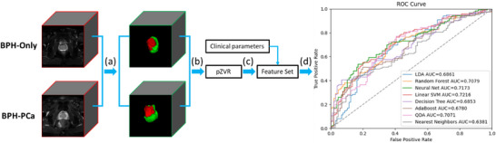
(a) Extraction of TZ&PZ in prostate MRIs using the pretrained ProZonaNet model, the detailed model architecture is illustrated in Figure 2. The input MRIs have been resampled to the fixed size of 128 × 128 × 32 voxels; (b) volume feature calculation based on the segmented results; (c) feature grouping and testing; (d) clinical validation.

2. METHODS

In Section 2.1 we describe the detailed structures of the presented 3D segmentation network ProZonaNet. In Section 2.2 we illustrate the details of the experimental design.

2.1. ProZonaNet for PZ and TZ segmentation

Training a GAN is challenging due to issues such as the imbalance between the generator and discriminator during training and the vanishing gradient problem affecting the generator. ³³ To address these challenges, we implemented a modified GAN architecture. Through extensive experimentation, we found that using a non‐skip connected encoder‐decoder architecture for the generator yields more stable training results.

We also employ a series of full pre‐activation residual blocks ¹⁴ for deep feature fusion and transition. The detailed schematic diagram of the presented ProZonaNet is shown in Figure 2.

FIGURE 2.

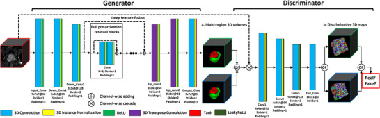
The detailed schematic diagram of ProZonaNet (The input, output, and annotation volumes are represented by red, green, and blue edged cubes, respectively. The 3D discriminative maps of the discriminator for synthetic or real regions of interest are also represented by green‐ and blue‐edged cubes, respectively).

2.1.1. Residual codec generator

The detailed structure of the generator is illustrated in the left part of Figure 2. The unique structure of GANs poses specific challenges during training. One such challenge is the strong classification ability of the discriminator, which can inhibit the backward gradient propagation to the generator. This inhibition often leads to the vanishing gradient problem in the generator, making the training process ineffective. This issue has been well‐documented in the literature. ³⁴ When designing effective GAN architecture, it is crucial to balance both the generator and discriminator modules. Through a series of controlled experiments, we discovered that incorporating skip connections from the shallow layers to the deep layers in the generator tends to exacerbate the gradient vanishing problem, leading to ineffective updates during training.

Therefore, we built a deep residual convolutional neural network‐based ³⁵ architecture as the generator. We use a series of pre‐activation residual blocks that have been shown to be the most promising ³⁶ as a bridge for feature fusion. The output layer of the generator uses the Tanh activation function to limit the range of predicted values to the range of [−1,1].

2.1.2. Customized Markov 3D patch discriminator

Inspired by PatchGAN, ²⁷ we develop a customized 3D Patch convolutional structure as the discriminator. The developed discriminator performs real or fake classification at the scale of local 3D patches, effectively modeling the 3D volume as a Markov random field, which functions as a texture/style loss.

The size of the input volume in the discriminator is 128 × 128 × 32. When the dilation size parameter of the convolutional layer is equal to 1, the output size O_size and the input size I_size of the convolutional layer have the following relationship:

$$O_{size}=\frac{I_{size}+2P-K}{S}+1$$ (1)

where P, K, and S represent padding size, convolutional kernel size, and stride size, respectively. According to Equation (1), the relationship between the receptive field (RF) of the i‐th convolutional layer and the RF of the previous convolutional layer can be backtracked as:

$$R{F}_i=\left(R{F}_{i-1}-1\right)s+k$$ (2)

Final experiments demonstrate that ProZonaNet can achieve the best performance when the RF size of the input layer is equal to 22 × 22 × 22. The detailed structure of the final fixed discriminator is illustrated in the right part of Figure 2.

2.1.3. Loss function

In contrast to Pix2pix, ProZonaNet does not need to synthesize diverse results, so the input to the generator does not need random noise. The final adversarial loss function of ProZonaNet is:

$$\begin{array}{cc}& {\mathcal{L}}_{cGAN}\left(G,D\right)\hfill \\ & =E_{x,y}\left[logD\left(x,y\right)\right]+E_x\left[\log \left(1-D\left(x,G\left(x\right)\right)\right)\right],\hfill \end{array}$$ (3)

where G and D represent the generator and the discriminator, x and y represent the input and target volumes, respectively. At the same time, to increase the stability of generator training, ProZonaNet adds L1 regularization loss as follows,

$${\mathcal{L}}_{\mathcal{l}1}\left(G\right)=E_{x,y}\left[{\left|\left|y-G\left(x\right)\right|\right|}_1\right]$$ (4)

The total optimization objective function is:

$$\underset{G}{\min }\underset{D}{\max }{\mathcal{L}}_{cGAN}\left(G,D\right)+\lambda {\mathcal{L}}_{l1}\left(G\right),$$ (5)

where λ is a parameter to control the weight of losses and was set to 10 in the experiments.

2.2. Experimental design

2.2.1. Data description and pre‐processing

Dataset

The dataset used in the experiment was obtained from Changhai Hospital, Shanghai, China. We leveraged N = 199 patient studies who underwent 3T multiparametric MRI followed by systematic/targeted biopsy with availability of clinical parameters including total prostate specific antigen (tPSA), patient age, gleason score (GS), and grade group. On biopsy, N = 106 patients were diagnosed with BPH‐Only and N = 93 was diagnosed with BPH‐PCa. The MRI scans were acquired with a Siemens 3T scanner with T2‐weighted sequences (voxel size of 0.7813 × 0.7813 × 3.5 mm). TZ and PZ annotations were obtained from a radiologist and a urologist, who collaboratively annotated and reviewed all 199 patient cases. The cohort was then randomly split into a training set (N = 139) and a test set (N = 60) with a 7:3 ratio. To enhance model generalizability and mitigate overfitting, data augmentation was applied to the training set, generating 973 augmented volumes through rotations (0°, 90°, 180°, 270° along the Z‐axis) and mirror flips along the X, Y, and Z axes. These augmented volumes were used to train ProZonaNet. Model evaluation was performed on the independent test set (N = 60), which contained no augmented samples, ensuring a fair and robust performance assessment.

Preprocessing steps

We leveraged T2W sequences in this study which underwent the following pre‐processing steps: (1) T2W intensity standardization: We compute a median template distribution of the T2W intensities to which all the scans are mapped and then automatically adjust the contrast according to 99% of the cumulative voxels; (2) Cropping to the prostate region of interest (ROI): A central cropping to the prostate ROI and consequently the PZ and TZ zones to a consistent size 192 pixels x 192 pixels × N, where N represents the number of slices in the axial view; (3) Resampling of the cropped T2W and corresponding ROI masks to a fixed size of 128 × 128 × 32; (4) Linear mapping of voxel values of T2W and annotations to the range of [0,1]; (5) Standardizing voxel values of MRIs and annotations to the interval of [−1, 1], using a mean of 0.5 and a variance of 0.5 to match the generator's output range. Following the processing of images by the ProZonaNet, post‐processing steps included (1) Remapping the voxel values of outputs from generator to the range of [0, 1] using a mean of 0.5 and a variance of 0.5; (2) Use the Multi‐Otsu Threshold algorithm ³⁷ to discretize the segmented results into three classes: 0, 1, and 2 represent background, TZ and PZ, respectively. The dataset description is in the Figure 3.

FIGURE 3.

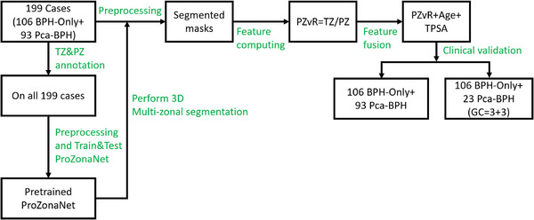
Patient selection chart and data description.

2.2.2. Experiment 1‐ Segmentation of prostate zonal volumes (PZ and TZ) on T2W MRI using ProZonaNet

Following pre‐processing, the T2W MRIs corresponding to BPH‐Only or BPH‐PCa are directly fed into the pretrained ProZonaNet model for TZ and PZ segmentation. We compared the segmentation performance of ProZonaNet with six state‐of‐the‐art (SOTA) 3D medical image segmentation networks, including 3DU‐net, ¹¹ 3DResU‐net, ¹³ HighRes‐net, ¹⁵ 3DDense‐net, ¹⁶ 3DDenseVoxel‐net, ¹⁷ V‐net. ¹⁸ All segmentation models were trained on 139 training cases (with augmentation) and evaluated on an independent test set of 60 cases (without augmentation), ensuring no data leakage. Segmentation performance was evaluated using Dice Similarity Coefficient (DSC) and Intersection over Union (IoU), providing a fair and standardized assessment of ProZonaNet's effectiveness in segmenting TZ and PZ regions on T2W MRI.

2.2.3. Experiment 2‐ Compute the prostate zonal volume ratio (pZVR) biomarker and evaluate its performance to distinguish BPH‐PCa from BPH‐Only

As previously mentioned, BPH tends to co‐occur with prostate cancer (BPH‐PCa), though in many cases BPH alone might be present with no evidence of prostate cancer (BPH‐Only). In this experiment, we calculated the pZVR as PZ/TZ obtained from the ProZonaNet to distinguish between BPH‐Only and BPH‐PCa. We also evaluated the performance of clinical parameters (tPSA, patient age, and prostate volume) via univariate and multivariate analysis in conjunction with pZVR. To assess the reliability and consistency of pZVR values computed using the ProZonaNet model, we applied the trained model—evaluated solely on the independent test set—to all 199 cases post‐validation. This application was used only for post hoc statistical correlation analyses, not for model training or inference benchmarking. We then compared pZVR values obtained from ProZonaNet's automatic segmentations against those derived from expert annotations. Statistical agreement was evaluated using the Concordance Correlation Coefficient (CCC), ³⁸ which measures both precision and accuracy of pZVR predictions. The results were illustrated in Figure 4.

FIGURE 4.

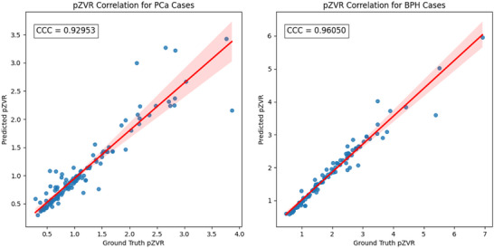
Concordance correlation coefficient (CCC) analysis for pZVR agreement between ProZonaNet‐derived values and ground truth annotations for PCa and BPH cases. The scatter plots illustrate the correlation between automatically computed and manually annotated pZVR values for BPH‐PCa cases (left) and BPH‐Only cases (right).

The results demonstrate a high correlation between ProZonaNet‐derived and manually annotated pZVR values, with CCC values of 0.929 for BPH‐PCa cases and 0.961 for BPH‐Only cases. Additionally, it suggests that ProZonaNet provides robust and reliable segmentation for computing pZVR, reinforcing its potential clinical utility in distinguishing BPH‐Only from BPH‐PCa. The image analysis pipeline, which includes prostate zonal segmentation, pZVR computation, and classification modeling, is summarized in Figure 1.

2.2.4. Computational parameters

ProZonaNet uses Adam ³⁹ as parameter optimizer. The initial learning rate of optimizer was set to 0.0002, and other parameters were set to default values. The model was implemented on Python 3.10.6 and Pytorch 1.12.1 library. The batch size of the training phase is 16 and the training epoch is 100. The main computing hardware includes one Nvidia GPU RTX 4090 with cuda v12.4 and Intel CPU Core (TM) i9‐ 14900K@3.20 GHz. Annotation and visualization of MRI data is done using ITK‐SNAP 3.6.0 ⁴⁰ software. The training hyperparameters of all models are summarized in Table S1.

3. RESULTS

3.1. Evaluation of prostate zone segmentations using ProZonaNet

3.1.1. Segmentation performance of ProZonaNet for PZ and TZ

ProZonaNet was trained using the augmented dataset consisting of 973 volumes, derived from 139 cases (Selected from 199 cases randomly) through data augmentation techniques. The model was evaluated on the independent test set of 60 cases only (without augmentation). The loss curve of ProZonaNet during the training phase is in Figure S1. Segmentation performance was assessed using mean Pixel Accuracy (mPA), mean Intersection Over Union (mIoU), mean Positive Predictive Value (mPPV), mean Dice Coefficient (mDICE), and mean Recall.

3.1.2. Comparison against state‐of‐the‐art (SOTA) segmentation methods

The SOTA models were trained and tested on the same dataset as ProZonaNet, and the comparative performance is illustrated in Table 1. The training curves for all SOTA models are in Figure S2.

TABLE 1.

Comparison of deep learning segmentation models on the independent test set (N = 60) for TZ and PZ segmentation.

	mPA	mIoU	mPPV	mDICE	mRecall
3DU‐net	0.997	0.780	0.833	0.868	0.895
3DResU‐net	0.996	0.718	0.860	0.847	0.846
HighRes‐net	0.996	0.789	0.878	0.814	0.889
3DDense‐net	0.996	0.714	0.885	0.820	0.841
3DDenseVoxel‐net	0.996	0.642	0.751	0.703	0.748
Vnet	0.996	0.751	0.895	0.865	0.874
ProZonaNet (presented)	0.998	0.858	0.921	0.925	0.920

The evaluation results show ProZonaNet achieved the highest segmentation performance among all models, with an mDICE of 0.925 and mIoU of 0.858, significantly outperforming state‐of‐the‐art 3D segmentation networks. Additionally, ProZonaNet demonstrated superior mPPV (0.921) and Recall (0.920), indicating its enhanced ability to accurately delineate prostate zones while maintaining robustness in capturing true positive regions.

To statistically validate the segmentation performance improvements of ProZonaNet, we computed 95% confidence intervals (CIs) and conducted paired t‐tests for the mDICE values of each model across the independent test set (N = 60). These analyses quantify both the consistency and statistical significance of model performance. The following Table 1a specifically summarizes the mean DICE scores and their corresponding 95% CIs for all models.

TABLE 1a.

Comparative statistical analysis of DICE scores with 95% confidence intervals (CI) and p values for ProZonaNet and baseline models.

	mDICE	p‐value	95% CIs
3DU‐net	0.868	7.224e‐30	(0.844, 0.892)
3DResU‐net	0.847	4.700e‐34	(0.821, 0.873)
HighRes‐net	0.814	2.441e‐36	(0.721, 0.846)
3DDense‐net	0.820	4.112e‐33	(0.791, 0.849)
3DDenseVoxel‐net	0.703	1.387e‐31	(0.665, 0.742)
Vnet	0.865	1.282e‐37	(0.842, 0.887)
ProZonaNet (presented)	0.925	*	(0.912, 0.938)

ProZonaNet achieved the highest mDICE score of 0.925 with a tight 95% confidence interval (CI) of (0.912, 0.938), indicating both strong accuracy and low variance in segmenting prostate zones. Statistical testing confirmed that these improvements were significant (p < 0.001) when compared to all baseline models, underscoring ProZonaNet's superior and consistent segmentation performance.

Additionally, to further evaluate the clinical relevance of segmentation quality, we conducted a comparative analysis examining how segmentation‐derived pZVR influences downstream classification performance. We recalculated the pZVR biomarker using segmentations from each of the six baseline models and ProZonaNet, then used these values in logistic regression models to distinguish BPH‐PCa from BPH‐Only cases. The comparative classification results are presented in Table 1b.

TABLE 1b.

Comparative classification performance using pZVR‐only derived from segmentation models and ground truth (N = 199).

	AUC	F1‐score	Precision	Recall	Accuracy
3DU‐net	0.759	0.726	0.667	0.797	0.677
3DResU‐net	0.753	0.731	0.676	0.796	0.686
HighRes‐net	0.712	0.703	0.634	0.783	0.687
3DDense‐net	0.726	0.714	0.631	0.821	0.645
3DDenseVoxel‐net	0.704	0.703	0.640	0.780	0.646
Vnet	0.755	0.753	0.689	0.829	0.707
ProZonaNet (presented)	0.769	0.760	0.696	0.837	0.716
GroundTruth	0.762	0.741	0.680	0.813	0.694

As shown in Table 1b, the pZVR derived from ProZonaNet achieved the highest AUC (0.769), F1‐score (0.760), and recall (0.837), outperforming all other segmentation‐based models and closely approximating the performance achieved using ground truth annotations. These findings demonstrate that improved segmentation accuracy directly enhances biomarker reliability and clinical classification performance, underscoring the value of ProZonaNet as both a robust segmentation model and an integral component of the newly presented imaging biomarker pipeline. Notably, while ground‐truth segmentations yield perfect spatial overlap (mDICE = 1.0), they may not always reflect the most biologically or functionally consistent zonal delineations due to inter‐observer variability and boundary ambiguity. In this context, such annotations should be considered a ‘silver standard’ rather than an absolute ground truth, as discussed in prior literature. ⁴¹ In contrast, ProZonaNet's outputs are trained to be spatially coherent and reproducible, leading to more stable volumetric features and greater robustness for downstream classification.

To further validate this observation, we conducted a paired statistical analysis comparing classification AUC values derived from each segmentation model against those from ground‐truth (GT) segmentations. Using identical test samples (N = 199), we performed paired t‐tests to assess whether the differences in classification performance were statistically significant. The results, summarized in Table S2, reveal that ProZonaNet's improvement over GT is statistically significant (p = 0.031), whereas differences for other models (e.g., VNet and 3DResU‐Net) did not reach statistical significance.

Illustration of PZ and TZ segmentations via 3DU‐net, 3DresU‐net, HighRes‐net, 3DDense‐net, 3DDenseVoxel‐net, Vnet, ProZonaNet, and Ground Truth are illustrated in Figure 5. We observe that ProZonaNet outperforms SOTA in terms of prostate peripheral and transition zone segmentations. Compared to the six state‐of‐the‐art (SOTA) 3D segmentation models, ProZonaNet achieves significantly higher mDICE scores, outperforming 3DU‐net, 3DResU‐net, HighRes‐net, 3DDense‐net, 3DDenseVoxel‐net, and VNet by 6.567%, 9.209%, 13.636%, 12.805%, 31.579%, and 6.936%, respectively.

FIGURE 5.

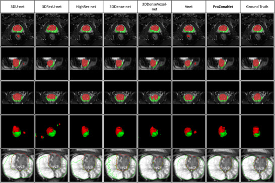
Prostate zonal segmentation results with ProZonaNet and comparison against other SOTA methods (From left to right, each column presents the mask from 3DU‐net, 3DResU‐net, HighRes‐net, 3DDense‐net, 3DDenseVoxel‐net, Vnet, ProZonaNet, and Ground Truth separately. Red and green represent the segmented transition and peripheral zones, respectively. The first four rows from top to bottom represent axial, Sagittal, coronal, and 3D views. The last row outlines the segmentation results of different models).

3.2. Evaluation of the prostate zonal volume ratio (pZVR) to distinguish BPH‐PCa and BPH‐Only

In this section, we use the same preprocessing steps for all N = 199 patients (106 BPH‐Only and 93 BPH‐PCa) and then feed the preprocessed cases into the pretrained ProZonaNet to get the corresponding TZ&PZ segmentation results. Finally, the pZVR (TZ/PZ) was calculated.

3.2.1. Statistical Methods

The effects of pZVR on the diagnosis of prostate cancer were estimated using univariate logistic regression, and their effects to distinguish tumor aggressiveness (prostate cancer vs. benign hyperplasia) were further estimated using a multivariable logistic regression model after controlling the effect of age and tPSA. The boxplot ⁴² of univariable analysis for pZVR is shown in Figure 6.

FIGURE 6.

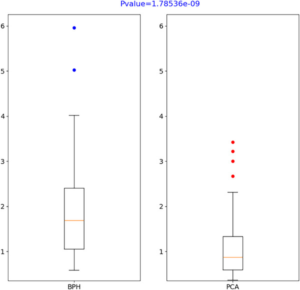
T‐test results of pZVR (pZVR was included in the multivariable logistic regression model and its added value on prostate cancer diagnosis was also estimated by the incremental value of AUC from two logistic regression models [one with and another without pZVR] through receiver operating characteristics [ROC] analysis. The optimal cutoff of the risk score to estimate the sensitivity and specificity was estimated by maximizing the Youden index. ⁴³ All tests are two‐sided and p values ≤ 0.05 were considered statistically significant.).

3.2.2. Results from univariate and multivariable regression analysis using logistic regression

From the univariate analysis, all factors/features were predictive of prostate cancer. According to the result in Table 2, the odds ratio for pZVR (OR = 0.291, 95% CI: 0.185–0.456, p < 0.0001) indicates that for each unit increase in pZVR, the odds of prostate cancer decrease significantly. After adjusting for age and tPSA in the multivariable analysis, pZVR remained a strong independent predictor of prostate cancer, with an even lower odds ratio (OR = 0.109, 95% CI: 0.055–0.217, p < 0.0001), highlighting its robustness in distinguishing BPH‐PCa from BPH‐Only. This finding highlights the utility of pZVR as a key predictive factor for distinguishing PCa from benign conditions. By incorporating pZVR, clinicians can more accurately identify patients at lower risk of clinically significant PCa, reducing false positives and unnecessary biopsies.

TABLE 2.

The effects of predictors on prostate cancer using logistic regression.

	Univariate		Multivariable
Factors	OR (95% CI)	p‐value	OR (95% CI)	p‐value
pZVR (= TZ/PZ) (per unit increase)	0.291 (0.185, 0.456)	<0.0001	0.109 (0.055, 0.217)	<0.0001
Age (per year increase)	1.118 (1.072, 1.166)	<0.0001	1.223 (1.147, 1.305)	<0.0001
tPSA (per ng/mL increase)	1.035 (1.011, 1.059)	0.003	1.037 (1.008, 1.067)	0.013

Abbreviations: CI, confidence interval; OR, odds ratio.

The interpretation of factors is the same. Each significant factor has clinical relevance:

1. pZVR (prostate zonal volume ratio): A unit increase in pZVR is associated with a 70.9% reduction in the odds of having prostate cancer in the univariate analysis (OR = 0.291, 95% CI: 0.185–0.456, p < 0.0001) and a 89.1% reduction after adjusting for age and tPSA in the multivariable analysis (OR = 0.109, 95% CI: 0.055–0.217, p < 0.0001). This demonstrates that a higher pZVR, often observed in BPH cases, is protective against prostate cancer.

2. Age: Each additional year of age increases the odds of prostate cancer by 11.8% in the univariate analysis (OR = 1.118, 95% CI: 1.072–1.166, p < 0.0001) and by 22.3% after adjustments (OR = 1.223, 95% CI: 1.147–1.305, p < 0.0001). This emphasizes age as a key risk factor.

3. tPSA (total prostate‐specific antigen): Each 1 ng/mL increase in tPSA is associated with 3.5% higher odds of prostate cancer both in univariate (OR = 1.035, 95% CI: 1.011–1.059, p = 0.003) and multivariable analyses (OR = 1.037, 95% CI: 1.008–1.067, p = 0.013), underscoring its role as a critical biomarker.

After controlling the effect of age and tPSA, pZVR remains a significant predictor of prostate cancer (OR = 0.109, p < 0.0001), highlighting its potential as a robust imaging biomarker for clinical use.

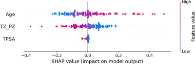
To illustrate how features contribute to the prediction of prostate cancer, we utilized SHAP (SHapley Additive exPlanations) analysis, ⁴⁴ which provides a quantitative measure of each feature's contribution to the model's output. SHAP values indicate whether a specific feature increases or decreases the likelihood of prostate cancer for a given patient, compared to the model's baseline prediction. Figure 7 displays a SHAP beeswarm plot comparing the contributions of TZ_PZ (pZVR) and clinical variables (age and tPSA) across all 199 patients (106 BPH‐Only and 93 BPH‐PCa).

FIGURE 7.

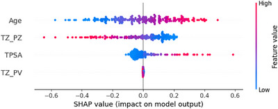
Feature importance visualization using SHAP values. The beeswarm plot illustrates the distribution of Shapley values, comparing the overall prediction importance of TZ_PZ and clinical variables across all 199 patients (106 BPH‐Only and 93 BPH‐PCa). Each point represents a variable's contribution to the prediction for an individual patient or sample. The plot demonstrates how each variable influences the model's output, either increasing or decreasing the prediction compared to the average.

In addition, a receiver operating characteristics (ROC) curve analysis (see also Figure 8 below) shows pZVR has good “diagnostic” performance with an incremental AUC of 0.169, which was a significant increase from AUC = 0.758 of the model with age and tPSA to AUC = 0.927 (p = 0.0001). The AUC value associated with pZVR reflects its strong predictive performance. This indicates that pZVR can reliably differentiate between PCa and BPH‐Only across the patient cohort (Figure 9).

FIGURE 8.

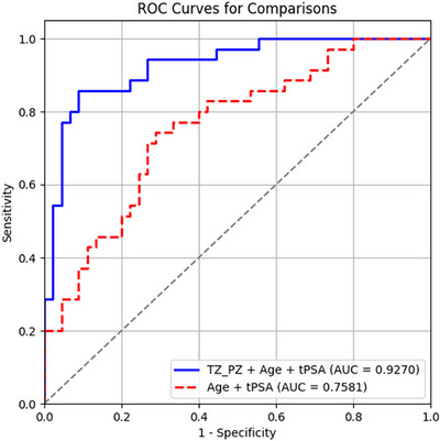
Inclusion of pZVR with clinical parameters (age, tPSA) improves distinguishing BPH‐PCa and BPH‐Only in comparison to clinical parameters alone. ROC curves from two models: TZ_PZ (pZVR) + age + tPSA (AUC = 0.927) and age + tPSA (AUC = 0.758).

FIGURE 9.

Feature importance analysis through SHAP values for distinguishing clinically insignificant BPH‐PCa cases. The beeswarm plot highlights the distribution of Shapley values, contrasting the predictive significance of pZVR and clinical variables between cases with GS = 3+3 or Grade Group = 1 (n = 23) and BPH‐Only (n = 106). Each point on the plot indicates how a particular variable contributes to the prediction for a single patient or sample. This visualization reveals the direction and magnitude of each variable's effect on the model's output, either augmenting or diminishing the predicted value relative to the mean.

3.3. Evaluation of pZVR in distinguishing low‐grade prostate cancer (Grade Group = 1) and BPH‐Only

To further analyze the effectiveness of the constructed pZVR in distinguishing BPH‐Only from low‐grade PCa, we identified a subset of patients with GS = 3+3 or Grade Group = 1 (n = 23) against BPH‐Only (n = 106).

From the univariate analysis, pZVR and age were predictive of prostate cancer. According to the result in Table 3, the odds ratio for pZVR (OR = 0.247, 95% CI: 0.106–0.574, p < 0.0001) indicates that for each unit increase in pZVR, the odds of prostate cancer decrease significantly. After controlling the effect of age (tPSA was dropped as it was not significant in the univariate analysis), pZVR still remained a strong independent predictor of prostate cancer, with an even lower odds ratio (OR = 0.113, 95% CI: 0.039–0.330, p < 0.0001), highlighting its robustness in distinguishing low‐grade BPH‐PCa from BPH‐Only.

TABLE 3.

The effects of predictors on prostate cancer (GS = 3 + 3) using logistic regression.

	Univariate		Multivariable
Factors	OR (95% CI)	p‐value	OR (95% CI)	p‐value
pZVR (= TZ/PZ) (per unit increase)	0.247 (0.106, 0.574)	0.001	0.113 (0.039, 0.330)	<0.0001
Age (per year increase)	1.105 (1.037, 1.177)	0.002	1.201 (1.103, 1.308)	<0.0001
tPSA (per ng/mL increase)	0.998 (0.954, 1.044)	0.932

Abbreviations: CI, confidence interval; OR, odds ratio.

In addition, a SHAP beeswarm plot and a ROC curve analysis (see Figure 9 and 10) show pZVR has good diagnostic performance with incremental improvement in AUC of 0.160 from AUC = 0.750 of the models with age alone to AUC = 0.910 (p = 0.002) with inclusion of pZVR.

FIGURE 10.

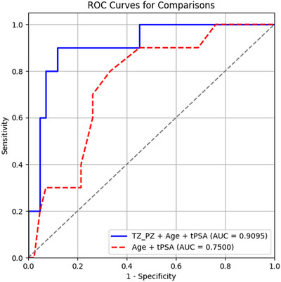
Addition of pZVR to clinical parameter (age) improves distinguishing GGG = 1 prostate cancer from BPH‐Only compared to age alone. ROC curves from two models: TZ_PZ (pZVR) + age (AUC = 0.910) and age (AUC = 0.750).

The evaluation of the pZVR biomarker demonstrates its strong clinical relevance and diagnostic capability in distinguishing BPH‐PCa from BPH‐Only cases. From the univariate logistic regression analysis in Table 2, pZVR exhibited a significant inverse relationship with prostate cancer risk, with an odds ratio (OR) of 0.291 (95% CI: 0.185‐0.456, p < 0.0001). This indicates that for every unit increase in pZVR, the odds of having prostate cancer decreased by 70.9%. When controlling for age and tPSA in multivariable analysis, pZVR remained a significant predictor, with an even lower OR of 0.109 (95% CI: 0.055–0.217, p < 0.0001). This highlights the robustness of pZVR as a predictor independent of other clinical variables. Furthermore, pZVR demonstrated high specificity in identifying low‐grade PCa cases, potentially reducing overdiagnosis and unnecessary biopsies.

4. DISCUSSION

The current imaging diagnosis of prostate cancer mainly relies on bi‐parametric MRI. ⁴⁵ However, many benign prostate diseases, such as BPH, have some degree of overlapping characteristics with PCa on MRI. This greatly reduces the diagnostic efficacy of MRI, necessitating invasive biopsies. This study investigates several key hypotheses:

Hypothesis 1

The development of a novel imaging biomarker for distinguishing BPH‐Only from BPH‐PCa and also can distinguish low‐grade PCa from BPH‐Only.

Hypothesis 2

A comparison of the segmentation performance between the presented ProzonaNet against SOTA models.

Hypothesis 3

The study includes both multivariate and univariate analyses to evaluate the diagnostic accuracy and clinical relevance of the proposed imaging biomarker.

In this study, we developed a GAN‐based 3D segmentation model (ProZonaNet) for automated and accurate segmentation of prostate zones, including the PZ and the TZ. Our segmentation model outperformed other SOTA segmentation models (including 3D UNet, VNet, and DenseNet‐based architectures). The segmentation model was used to compute the pZVR for distinguishing between BPH‐Only and BPH‐PCa, resulting in the best performance when integrated with clinical parameters (age and PSA), compared to using clinical parameters alone.

Distinguishing BPH‐Only and BPH‐PCa on MRI has been previously explored using computationally derived texture features. For instance, Xing et al. ⁴⁶ evaluated the role of radiomic texture features on T2W‐MRI and apparent diffusion coefficient (ADC) maps to distinguish BPH‐Only and BPH‐PCa and demonstrated promising results. Similarly, Gui et al. ⁴⁷ demonstrated the value of radiomics from MRI to distinguish BPH‐Only and BPH‐PCa, reporting promising results. However, radiomic texture features are susceptible to site and scanner‐specific variations. ⁴⁸ The pZVR biomarker presented in this study is independent of the artifacts commonly associated with MRI scans, including bias field and intensity drift issues, and hence less sensitive to intensity variations compared to textural parameters.

Previous studies have shown that prostatic PZ and TZ volumes are associated with BPH‐Only and BPH‐PCa. A previous study led by Bo et al. ⁴⁹ has shown that PSA and prostate volumes play a significant role in identifying benign and malignant lesions in the prostate. Sellers et al. ⁵⁰ suggested that patients with BPH‐Only had higher full prostate volumes compared to those without BPH‐Only. Yang et al. ⁵¹ showed that patients with larger PZ volume on MRI tend to have a high‐grade PCa, while those with higher TZ volume tend to be impacted by low‐grade PCa. These studies suggest that zonal volumes of the prostate on MRI tend to have strong associations with the incidence of BPH‐Only versus BPH‐PCa. We demonstrated in our study that the ratio of TZ to the total prostate volume (PV) and TZ to the PZ was differentially expressed between patients with BPH‐Only versus BPH‐PCa. The ratio of TZ to PV captures the relative volume of TZ, and a higher ratio suggests a higher TZ. As indicated in Figure 6, we observed that the TZ/PV ratio was higher in patients with BPH‐PCa compared to BPH‐Only.

We also demonstrated in our study that the addition of clinical parameters, including PSA, age, to pZVR resulted in the best discriminating classifier distinguishing BPH‐Only and BPH‐PCa. Particularly in the context of low‐grade BPH‐PCa and BPH‐Only, which tend to have maximum overlapping characteristics, ⁵² we demonstrated that the addition of pZVR improved distinguishing BPH‐Only and BPH‐PCa on a subset of patient studies.

Based on our experimental results, the pZVR represents a significant advancement in distinguishing low‐grade prostate cancer (PCa) from benign prostatic hyperplasia (BPH). Although biparametric prostate MRI may not reliably detect low‐grade PCa (Gleason Score 3+3), ⁴⁵ this limitation is generally acceptable, as many low‐grade cases do not require immediate treatment, and asymptomatic BPH often requires no intervention. However, low‐grade PCa still necessitates careful risk stratification. Active surveillance has shown promising outcomes for low‐grade PCa, with 76% of patients remaining treatment‐free at 5 years and only a 0.6% risk of metastasis at 10 years. However, Epstein's studies reveal that Gleason score alone is insufficient for selecting patients for active surveillance. ⁵³ Even with a Gleason Score of 3+3, tumor volumes greater than 0.5 cm³ are associated with adverse pathological features, such as higher stage, positive surgical margins, lymph node involvement, and perineural invasion. This suggests that some cases, seemingly low‐risk cancers, may benefit from definitive treatment. ⁵⁴ , ⁵⁵ The pZVR offers two key clinical advantages: (1) It could reduce unnecessary biopsies in BPH cases, thereby minimizing complications like infection, bleeding, and sepsis.(2) When combined with total PSA and age, it could enhance risk assessment for low grade PCa, leading to improved management strategy selection. Specifically, pZVR improves diagnostic specificity by effectively distinguishing low‐grade PCa from BPH‐Only, reducing false positives and unnecessary interventions. This specificity is crucial in avoiding overtreatment of indolent tumors that do not require aggressive management. Derived from MR imaging, pZVR offers a non‐invasive alternative to traditional diagnostic approaches, minimizing patient discomfort and risks associated with invasive procedures such as biopsies. By identifying patients with low‐grade PCa or benign conditions, pZVR can help guide clinicians in adopting a more conservative “active surveillance” strategy, supporting personalized and precise treatment plans. Additionally, pZVR, as a novel imaging‐derived biomarker, has the potential to complement traditional clinical biomarkers such as tPSA and radiomic features, offering a multi‐dimensional diagnostic approach. Integrating pZVR with these established factors could enhance risk stratification and provide a more comprehensive diagnostic profile, ultimately improving personalized treatment management. Our results demonstrate that pZVR remains a significant predictor of prostate cancer after adjusting for age and total PSA, with an odds ratio of 0.109 (p < 0.0001), indicating that higher TZ/PZ ratios are associated with lower cancer probability. Interestingly, while pZVR demonstrates an inverse relationship with cancer risk (OR = 0.291, p < 0.0001), age shows a stronger positive association (OR = 1.118, p < 0.0001). These findings suggest that although the TZ/PZ ratio typically increases with age, the age‐related increase in cancer risk outweighs the protective effect of higher pZVR values. The approach employed in ProZonaNet and pZVR could be extended to other medical imaging contexts where segmentation and ratio‐based biomarkers provide diagnostic value. For instance, in chronic liver disease, the caudate‐to‐right lobe ratio (C/RL) has been validated as an imaging biomarker for assessing cirrhosis, achieving an AUC of 0.797. A threshold of >0.90 for C/RL demonstrates 71.7% sensitivity, 77.4% specificity, and 74.2% accuracy in diagnosing cirrhosis. ⁵⁶ Similarly, zone‐based analysis may be beneficial in evaluating structural changes that precede clinical symptoms, such as white matter‐to‐gray matter ratios in neurodegenerative diseases ⁵⁷ or cortex‐to‐medulla ratios in chronic kidney disease. ⁵⁸ Future research could focus on adapting ProZonaNet's deep learning framework to these and other applications, leveraging anatomical ratios as key biomarkers for improved diagnostic and prognostic precision.

Although our study presents promising results, it is crucial to acknowledge certain limitations. Firstly, the performance evaluation and validation primarily relied on a single institution dataset, potentially limiting the generalizability of our findings across diverse clinical settings. Secondly, the performance of ProZonaNet is inherently influenced by the quality of MRI scans and the accuracy of expert annotations. Variability in segmentation accuracy may arise due to MRI artifacts, such as motion blur or noise, which can affect image clarity and the reliability of the model's predictions. ⁵⁹ At the same time, inconsistencies in annotation practices across institutions, stemming from differences in radiologists’ expertise or interpretation of ambiguous boundaries, may introduce bias into the training process. ⁶⁰

Although we employed a rigorous training strategy, the development of the segmentation model might benefit from further validation with larger datasets and varied patient populations, including PCa. Finally, we were limited to exploring PSA and age as the clinical parameters of interest. Other factors, such as PI‐RADS score, were not included in our study since none of the patients with a PI‐RADS score of less than 3 were biopsied for cancer. Further exploration and validation across broader datasets are necessary to ensure its applicability in real‐world clinical scenarios.

Our future endeavors include expanding the application of ProZonaNet across multiple 3D medical segmentation datasets to validate its robustness and improve clinical utility. Additionally, we will focus on developing strategies to mitigate these limitations, such as incorporating domain adaptation techniques ⁴⁴ to handle variability across datasets and employing ensemble learning approaches to improve model robustness against annotation inconsistencies.

CONFLICT OF INTEREST STATEMENT

Dr. Anant Madabhushi is a Research Career Scientist at the Atlanta Veterans Affairs Medical Center. He is an equity holder in Picture Health, Elucid Bioimaging, and Inspirata Inc., and currently serves on the advisory board of Picture Health. He consults for Takeda Inc. and has sponsored research agreements with AstraZeneca and Bristol Myers‐Squibb. His technology has been licensed to Picture Health and Elucid Bioimaging. He is also involved in one NIH R01 grant with Inspirata Inc. All other authors declare no competing financial interests.

Supporting information

Supporting Information

Zhang Z, Yang Q, Shiradkar R, et al. A deep learning derived prostate zonal volume‐based biomarker from T2‐weighted MRI to distinguish between prostate cancer and benign prostatic hyperplasia. Med. Phys.. 2025;52:e18053. 10.1002/mp.18053

REFERENCES

- 1. Siegel RL, Miller KD, Wagle NS, Jemal A. Cancer statistics, 2023. Ca Cancer J Clin. 2023;73(1):17‐48. [DOI] [PubMed] [Google Scholar]
- 2. Quon JS, Moosavi B, Khanna M, Flood TA, Lim CS, Schieda N. False positive and false negative diagnoses of prostate cancer at multi‐parametric prostate MRI in active surveillance. Insights Imaging. 2015;6(4):449‐463. doi: 10.1007/s13244-015-0411-3 [DOI] [PMC free article] [PubMed] [Google Scholar]
- 3. Kitzing YX, Prando A, Varol C, Karczmar GS, Maclean F, Oto A. Benign conditions that mimic prostate carcinoma: MR imaging features with histopathologic correlation. Radiographics. 2016;36(1):162‐175. doi: 10.1148/rg.2016150030 [DOI] [PMC free article] [PubMed] [Google Scholar]
- 4. Engelbrecht MR, Huisman HJ, Laheij RJF, et al. Discrimination of prostate cancer from normal peripheral zone and central gland tissue by using dynamic contrast‐enhanced MR imaging. Radiology. 2003;229(1):248‐254. doi: 10.1148/radiol.2291020200 [DOI] [PubMed] [Google Scholar]
- 5. Vargas HA. Normal central zone of the prostate and central zone involvement by prostate cancer: clinical and MR imaging implications. Radiology. 2012;264(2):617‐617. (vol 262, pg 894, 2012). [DOI] [PMC free article] [PubMed] [Google Scholar]
- 6. Hosseinzadeh K, Schwarz SD. Endorectal diffusion‐weighted imaging in prostate cancer to differentiate malignant and benign peripheral zone tissue. Magn Reson Imaging. 2004;20(4):654‐661. doi: 10.1002/jmri.20159 [DOI] [PubMed] [Google Scholar]
- 7. Chang Y, Chen R, Yang Q, et al. Peripheral zone volume ratio (PZ‐ratio) is relevant with biopsy results and can increase the accuracy of current diagnostic modality. Oncotarget. 2017;8(21):34836‐34843. doi: 10.18632/oncotarget.16753 [DOI] [PMC free article] [PubMed] [Google Scholar]
- 8. Klein S, van der Heide UA, Lips IM, van Vulpen M, Staring M, Pluim JPW. Automatic segmentation of the prostate in 3D MR images by atlas matching using localized mutual information. Med Phys. 2008;35(4):1407‐1417. doi: 10.1118/1.2842076 [DOI] [PubMed] [Google Scholar]
- 9. Makni N, Iancu A, Colot O, Puech P, Mordon S, Betrouni N. Zonal segmentation of prostate using multispectral magnetic resonance images. Med Phys. 2011;38(11):6093‐6105. doi: 10.1118/1.3651610 [DOI] [PubMed] [Google Scholar]
- 10. Litjens G, Debats O, Van De Ven W, Karssemeijer N, Huisman H. A pattern recognition approach to zonal segmentation of the prostate on MRI. In: Ayache N, Delingette H, Golland P, Mori K, eds. Medical Image Computing and Computer‐Assisted Intervention—MICCAI 2012. Springer; 2012:413‐420. doi: 10.1007/978-3-642-33418-4_51. Lecture Notes in Computer Science. [DOI] [PubMed] [Google Scholar]
- 11. Çiçek Ö, Abdulkadir A, Lienkamp SS, Brox T, Ronneberger O. 3D U‐Net: Learning Dense Volumetric Segmentation From Sparse Annotation. Published online June 21, 2016. doi: 10.48550/arXiv.1606.06650 [DOI]
- 12. Ronneberger O, Fischer P, Brox T. U‐Net: convolutional networks for biomedical image segmentation. In: Navab N, Hornegger J, Wells WM, Frangi AF, eds. Medical Image Computing and Computer‐Assisted Intervention—MICCAI 2015. Springer International Publishing; 9351:234‐241. doi: 10.1007/978-3-319-24574-4_28. Lecture Notes in Computer Science. [DOI] [Google Scholar]
- 13. Rassadin A. Deep residual 3D U‐Net for joint segmentation and texture classification of nodules in lung. In: Campilho A, Karray F, Wang Z, eds. Image Analysis and Recognition. Springer International Publishing; 2020:419‐427. doi: 10.1007/978-3-030-50516-5_37. Lecture Notes in Computer Science. [DOI] [Google Scholar]
- 14. He K, Zhang X, Ren S, Sun J, Deep residual learning for image recognition. In: Proceedings of the IEEE Conference on Computer Vision and Pattern Recognition ; 2016:770‐778. Accessed June 12, 2024. http://openaccess.thecvf.com/content_cvpr_2016/html/He_Deep_Residual_Learning_CVPR_2016_paper.html
- 15. Li W, Wang G, Fidon L, Ourselin S, Cardoso MJ, Vercauteren T. On the compactness, efficiency, and representation of 3D convolutional networks: brain parcellation as a pretext task. In: Niethammer M, Styner M, Aylward S, eds. Information Processing in Medical Imaging. Springer International Publishing; 2017:348‐360. doi: 10.1007/978-3-319-59050-9_28. Lecture Notes in Computer Science. [DOI] [Google Scholar]
- 16. Bui TD, Shin J, Moon T, 3D Densely Convolutional Networks for Volumetric Segmentation. Published online September 13, 2017. Accessed June 12, 2024. http://arxiv.org/abs/1709.03199
- 17. Yu L, Cheng JZ, Dou Q. Automatic 3D cardiovascular MR segmentation with densely‐connected volumetric ConvNets. In: Descoteaux M, Maier‐Hein L, Franz A, Jannin P, Collins DL, Duchesne S, eds. Medical Image Computing and Computer‐Assisted Intervention − MICCAI 2017. Springer International Publishing; 2017:287‐295. doi: 10.1007/978-3-319-66185-8_33. Lecture Notes in Computer Science. [DOI] [Google Scholar]
- 18. Milletari F, Navab N, Ahmadi SA, V‐net: fully convolutional neural networks for volumetric medical image segmentation. In: 2016 Fourth International Conference on 3D Vision (3DV) . Ieee; 2016:565‐571. Accessed June 12, 2024. https://ieeexplore.ieee.org/abstract/document/7785132/ [Google Scholar]
- 19. Hashemi SR, Mohseni Salehi SS, Erdogmus D, Prabhu SP, Warfield SK, Gholipour A. Asymmetric loss functions and deep densely‐connected networks for highly‐imbalanced medical image segmentation: application to multiple sclerosis lesion detection. IEEE Access. 2019;7:1721‐1735. doi: 10.1109/ACCESS.2018.2886371 [DOI] [PMC free article] [PubMed] [Google Scholar]
- 20. El Jurdi R, Petitjean C, Honeine P, Cheplygina V, Abdallah F. High‐level prior‐based loss functions for medical image segmentation: a survey. Comput Vision Image Understanding. 2021;210:103248. doi: 10.1016/j.cviu.2021.103248 [DOI] [Google Scholar]
- 21. Salehi SSM, Erdogmus D, Gholipour A. Tversky loss function for image segmentation using 3D fully convolutional deep networks. In: Wang Q, Shi Y, Suk HI, Suzuki K, eds. Machine Learning in Medical Imaging. Springer International Publishing; 2017:379‐387. doi: 10.1007/978-3-319-67389-9_44 [DOI] [Google Scholar]
- 22. Goodfellow I, Pouget‐Abadie J, Mirza M, et al. Generative adversarial networks. Commun ACM. 2020;63(11):139‐144. doi: 10.1145/3422622 [DOI] [Google Scholar]
- 23. Yan W, Wang Y, Gu S. The domain shift problem of medical image segmentation and vendor‐adaptation by Unet‐GAN. In: Shen D, Liu T, Peters TM, eds. Medical Image Computing and Computer Assisted Intervention—MICCAI 2019. Springer International Publishing; 2019:623‐631. doi: 10.1007/978-3-030-32245-8_69. Lecture Notes in Computer Science. [DOI] [Google Scholar]
- 24. Xun S, Li D, Zhu H, et al. Generative adversarial networks in medical image segmentation: a review. Comput Biol Med. 2022;140:105063. [DOI] [PubMed] [Google Scholar]
- 25. Han C, Hayashi H, Rundo L, et al. GAN‐based synthetic brain MR image generation. In: 2018 IEEE 15th International Symposium on Biomedical Imaging (ISBI2018) . IEEE; 2018:734‐738. Accessed June 12, 2024. https://ieeexplore.ieee.org/abstract/document/8363678/ [Google Scholar]
- 26. Sun Y, Yuan P, Sun Y, MM‐GAN: 3D MRI data augmentation for medical image segmentation via generative adversarial networks. In: 2020 IEEE International Conference on Knowledge Graph (ICKG) . IEEE; 2020:227‐234. Accessed June 12, 2024. https://ieeexplore.ieee.org/abstract/document/9194564/ [Google Scholar]
- 27. Isola P, Zhu JY, Zhou T, Efros AA, Image‐to‐image translation with conditional adversarial networks. In: Proceedings of the IEEE Conference on Computer Vision and Pattern Recognition ; 2017:1125‐1134.
- 28. Mirza M, Osindero S, Conditional Generative Adversarial Nets. Published online November 6, 2014. Accessed June 12, 2024. http://arxiv.org/abs/1411.1784
- 29. Eslami M, Tabarestani S, Albarqouni S, Adeli E, Navab N, Adjouadi M. Image‐to‐images translation for multi‐task organ segmentation and bone suppression in chest x‐ray radiography. IEEE Trans Med Imaging. 2020;39(7):2553‐2565. [DOI] [PubMed] [Google Scholar]
- 30. Popescu D, Deaconu M, Ichim L, Stamatescu G, Retinal blood vessel segmentation using pix2pix gan. In: 2021 29th Mediterranean Conference on Control and Automation (MED) . IEEE; 2021:1173‐1178. Accessed June 12, 2024. https://ieeexplore.ieee.org/abstract/document/9480169/ [Google Scholar]
- 31. Cirillo MD, Abramian D, Eklund A. Vox2Vox: 3D‐GAN for brain tumour segmentation. In: Crimi A, Bakas S, eds. Brainlesion: Glioma, Multiple Sclerosis, Stroke and Traumatic Brain Injuries. Springer International Publishing; 2021:274‐284. doi: 10.1007/978-3-030-72084-1_25 [DOI] [Google Scholar]
- 32. Mahmood F, Borders D, Chen RJ, et al. Deep adversarial training for multi‐organ nuclei segmentation in histopathology images. IEEE Trans Med Imaging. 2019;39(11):3257‐3267. [DOI] [PMC free article] [PubMed] [Google Scholar]
- 33. Goodfellow I. NIPS 2016 Tutorial: Generative Adversarial Networks. Published online April 3, 2017. Accessed June 12, 2024. http://arxiv.org/abs/1701.00160
- 34. Sajeeda A, Hossain BMM. Exploring generative adversarial networks and adversarial training. Int J Cogn Comput Eng. 2022;3:78‐89. doi: 10.1016/j.ijcce.2022.03.002 [DOI] [Google Scholar]
- 35. Johnson J, Alahi A, Fei‐Fei L. Perceptual losses for real‐time style transfer and super‐resolution. In: Computer Vision–ECCV2016: 14th European Conference, Amsterdam, The Netherlands, October 11–14, 2016, Proceedings, Part II 14 . Springer; 2016:694‐711. [Google Scholar]
- 36. He K, Zhang X, Ren S, Sun J. Identity mappings in deep residual networks. In: Leibe B, Matas J, Sebe N, Welling M, eds. Computer Vision—ECCV 2016. Springer International Publishing; 2016:630‐645. doi: 10.1007/978-3-319-46493-0_38. Lecture Notes in Computer Science. [DOI] [Google Scholar]
- 37. Liao PS, Chen TS, Chung PC. A fast algorithm for multilevel thresholding. J Inf Sci Eng. 2001;17(5):713‐727. [Google Scholar]
- 38. Lawrence I, Lin K. A concordance correlation coefficient to evaluate reproducibility. Biometrics. 1989:255‐268. [PubMed] [Google Scholar]
- 39. Kingma DP, BaJ Adam: A method for stochastic optimization. arXiv preprint arXiv:14126980. Published online 2014.
- 40. Yushkevich PA, Gao Y, Gerig G. ITK‐SNAP: an interactive tool for semi‐automatic segmentation of multi‐modality biomedical images. In: 2016 38th Annual International Conference of the IEEE Engineering in Medicine and Biology Society (EMBC) . IEEE; 2016:3342‐3345. Accessed June 12, 2024. https://ieeexplore.ieee.org/abstract/document/7591443/ [DOI] [PMC free article] [PubMed] [Google Scholar]
- 41. Wagholikar KB, Estiri H, Murphy M, Murphy SN. Polar labeling: silver standard algorithm for training disease classifiers. Bioinformatics. 2020;36(10):3200‐3206. [DOI] [PMC free article] [PubMed] [Google Scholar]
- 42. Williamson DF. The box plot: a simple visual method to interpret data. Ann Intern Med. 1989;110(11):916. doi: 10.7326/0003-4819-110-11-916 [DOI] [PubMed] [Google Scholar]
- 43. Fluss R, Faraggi D, Reiser B. Estimation of the Youden index and its associated cutoff point. Biom J. 2005;47(4):458‐472. doi: 10.1002/bimj.200410135 [DOI] [PubMed] [Google Scholar]
- 44. Wilson G, Cook DJ. A survey of unsupervised deep domain adaptation. ACM Trans Intell Syst Technol. 2020;11(5):1‐46. [DOI] [PMC free article] [PubMed] [Google Scholar]
- 45. Belue MJ, Yilmaz EC, Daryanani A, Turkbey B. Current status of biparametric MRI in prostate cancer diagnosis: literature analysis. Life (Basel). 2022;12(6):804. doi: 10.3390/life12060804 [DOI] [PMC free article] [PubMed] [Google Scholar]
- 46. Xing P, Chen L, Yang Q, et al. Differentiating prostate cancer from benign prostatic hyperplasia using whole‐lesion histogram and texture analysis of diffusion‐ and T2‐weighted imaging. Cancer Imaging. 2021;21(1):54. doi: 10.1186/s40644-021-00423-5 [DOI] [PMC free article] [PubMed] [Google Scholar]
- 47. Gui S, Lan M, Wang C, Nie S, Fan B. Application value of radiomic nomogram in the differential diagnosis of prostate cancer and hyperplasia. Front Oncol. 2022;12:859625. [DOI] [PMC free article] [PubMed] [Google Scholar]
- 48. Liu X, Maleki F, Muthukrishnan N, et al. Site‐specific variation in radiomic features of head and neck squamous cell carcinoma and its impact on machine learning models. Cancers (Basel). 2021;13(15):3723. doi: 10.3390/cancers13153723 [DOI] [PMC free article] [PubMed] [Google Scholar]
- 49. Bo M, Ventura M, Marinello R, Capello S, Casetta G, Fabris F. Relationship between prostatic specific antigen (PSA) and volume of the prostate in the benign prostatic hyperplasia in the elderly. Crit Rev Oncol Hematol. 2003;47(3):207‐211. [DOI] [PubMed] [Google Scholar]
- 50. Sellers J, Wagstaff RG, Helo N, De Riese WTW. Quantitative measurements of prostatic zones by MRI and their dependence on prostate size: possible clinical implications in prostate cancer. Ther Adv Urol. 2021;13:175628722110008. doi: 10.1177/17562872211000852 [DOI] [PMC free article] [PubMed] [Google Scholar]
- 51. Yang L, Li M, Zhang MN, Yao J, Song B. Association of prostate zonal volume with location and aggressiveness of clinically significant prostate cancer: a multiparametric MRI study according to PI‐RADS version 2.1. Eur J Radiol. 2022;150:110268. [DOI] [PubMed] [Google Scholar]
- 52. Żurowska A, Pęksa R, Bieńkowski M, et al. Prostate cancer and its mimics—a pictorial review. Cancers (Basel). 2023;15(14):3682. doi: 10.3390/cancers15143682 [DOI] [PMC free article] [PubMed] [Google Scholar]
- 53. Carlsson S, Benfante N, Alvim R, et al. Long‐term outcomes of active surveillance for prostate cancer: the memorial sloan kettering cancer center experience. J Urol. 2020;203(6):1122‐1127. [DOI] [PMC free article] [PubMed] [Google Scholar]
- 54. Epstein JI, Carmichael M, Partin AW, Walsh PC. Is tumor volume an independent predictor of progression following radical prostatectomy? A multivariate analysis of 185 clinical stage B adenocarcinomas of the prostate with 5 years of followup. J Urol. 1993;149(6):1478‐1481. [DOI] [PubMed] [Google Scholar]
- 55. Ghiasy S, Abedi AR, Moradi A, et al. Is active surveillance an appropriate approach to manage prostate cancer patients with Gleason Score 3+3 who met the criteria for active surveillance? Turk J Urol. 2019;45(4):261‐264. [DOI] [PMC free article] [PubMed] [Google Scholar]
- 56. Awaya H, Mitchell DG, Kamishima T, Holland G, Ito K, Matsumoto T. Cirrhosis: modified caudate‐right lobe ratio. Radiology. 2002;224(3):769‐774. [DOI] [PubMed] [Google Scholar]
- 57. Tamagaki C, Sedvall GC, Jönsson EG, et al. Altered white matter/gray matter proportions in the striatum of patients with schizophrenia: a volumetric MRI study. Am J Psychiatry. 2005;162(12):2315‐2321. [DOI] [PubMed] [Google Scholar]
- 58. Korfiatis P, Denic A, Edwards ME, et al. Automated segmentation of kidney cortex and medulla in CT images: A multisite evaluation study. J Am Soc Nephrol. 2022;33(2):420‐430. [DOI] [PMC free article] [PubMed] [Google Scholar]
- 59. Wells WM, Grimson WE, Kikinis R, Jolesz FA. Adaptive segmentation of MRI data. IEEE Trans Med Imaging. 1996;15(4):429‐442. [DOI] [PubMed] [Google Scholar]
- 60. Chen J, Gandomkar Z, Reed WM. Investigating the impact of cognitive biases in radiologists’ image interpretation: a scoping review. Eur J Radiol. 2023:111013. [DOI] [PubMed] [Google Scholar]
Associated Data
This section collects any data citations, data availability statements, or supplementary materials included in this article.
Supplementary Materials