Spectral phasor imaging on a commercial confocal microscope without a spectral detector

Abstract

Spectral imaging is a fluorescence microscopy technique with several applications, including imaging of environment-sensitive probes, spectral unmixing and identification of fluorescent species. In confocal microscopes not equipped with a spectral detection unit, spectral images can be obtained using the lambda scan mode of the microscope, namely the sequential acquisition of images using a tunable emission filter or other dispersive optical elements. Unfortunately, the lambda scan mode has poor temporal resolution, is a photon-wasting technique, and is not ideal for the spectral imaging of live samples. Here, we describe a spectral imaging method that can be implemented on commercial confocal microscopes not equipped with a spectral detector. The method is based on simultaneous image acquisition in 4 contiguous spectral channels and spectral phasor analysis. We demonstrate that this method can be easily implemented on a Leica confocal laser scanning microscope, with better photon efficiency and temporal resolution than the lambda scan mode. We perform a 4-channel (4 C) spectral phasor analysis of live cells stained with the environment-sensitive ACDAN and Nile Red dyes. We can distinguish changes in spectral emission in the order of 5 nm between different subcellular compartments. We show that 4 C-spectral phasor can be used to decompose the Nile Red signal into 2 components and perform 3-color imaging in combination with a DNA dye in live organoids. Finally, we show that the 4 C-spectral phasor can be also used to unmix the signal of fluorescent proteins with overlapping emission spectra such as mEmerald and EYFP.

Introduction

Spectral imaging is a fluorescence microscopy technique in which the emission spectrum is obtained at each pixel of an image. Spectral imaging has several applications, including imaging of environment-sensitive probes, spectral unmixing, and identification of fluorescent species^1–4. Spectral imaging involves, in the simplest case, the collection of a dataset of the type I(x, y,λ), sometimes called a cube or lambda-stack. The acquisition modalities can be broadly classified as spectral scanning, spatial scanning or snapshot methods. Confocal microscopy is intrinsically a point scanning technique where a raster scan of the sample forms the image. In confocal microscopy, spectral scanning is typically achieved by substituting the emission filter with a tunable filter and serially acquiring images at different emission wavelengths. This is also called wavelength scan or lambda scan acquisition mode and is available in many commercial setups^5–7. Unfortunately, the temporal resolution of this approach is quite poor (limited by the raster and spectral scans) and all the fluorescence photons not selected by the tunable filter are wasted. Thus, lambda scan is a time- and photon-consuming technique, not ideal for the spectral imaging of live samples. A faster alternative is provided by spatial scanning. In confocal microscopy, fast spectral imaging can be performed by substituting the standard point-detector with a spectral detector. The spectral detector is essentially a dispersive element, such as a prism or grating, placed before a multichannel detector. The spectral detector enables the acquisition of emission spectra at each pixel of an image, without affecting the temporal resolution of the confocal microscope. Examples of commercially available spectral detector systems are the Zeiss Meta and QUASAR detection units^7,8 or the Nikon A1-DUS spectral detector unit^9,10. Thus, the spectral detector provides fast spectral imaging but is not available on any confocal microscope.

The phasor approach was originally developed and extensively applied for the analysis of fluorescence lifetime images^11,12. The phasor analysis is currently used in many other applications, including spectral/hyperspectral imaging^13–20 and super-resolution microscopy^21–24. In particular, the spectral phasor approach was introduced to provide a simple and intuitive framework for the analysis of spectral imaging data^25,26. The phasor is a simplified frequency-domain approach where the temporal or spectral information at each pixel is Fourier-transformed to get the real and imaginary component g(x, y) and s(x, y), which represent the cartesian coordinates of the phasor¹⁴. Spectral differences between pixels are easily detected as differences in the position of the phasor. Pixels with similar spectra tend to cluster in the phasor plot whereas pixels with different spectra tend to separate in the same plot.

Here, we show a spectral phasor analysis of multi-color images acquired with a commercial confocal laser scanning microscope not equipped with a spectral detector. The images are obtained by simultaneous acquisition in 4 detection channels of a Leica SP8 or STELLARIS8 microscope, so that the temporal resolution is preserved, and photons are not wasted. The typical dataset is a 4-colors image where the 4 channels correspond to contiguous spectral bands with a bin width of 50 nm. Considering that typical fluorophore emission spectra have widths in the order of 100 nm, this spectral bandwidth provides sufficient sampling of the spectrum’s shape. An advantage of this approach is the much higher temporal resolution, compared with the lambda scan mode of the same microscope. The spectral information can be visualized using the phasor plot and phase-wavelength images. We perform 4-channel (4 C) spectral phasor analysis of the environment-sensitive ACDAN and Nile Red dyes in live cells and organoids. We show that we can distinguish shifts in spectral emission in the order of 5 nm between different subcellular compartments. The 4 C-spectral phasor can be used to decompose the Nile Red signal into 2 components and perform 3-color imaging in combination with Hoechst in live organoids. We also show spectral unmixing of the fluorescent proteins mEmerald and EYFP in live cells. The proposed method can be useful for performing fast and photon-efficient spectral imaging in confocal microscopes without spectral detection units.

Materials and methods

Preparation of fluorescent probe solutions

A solution of the fluorophore ANS in presence of Bovine Serum Albumin (BSA) (ANS-BSA) was prepared by adding 3% BSA (Sigma-Aldrich, A7030) to a ~ 250 µM water solution of ANS (Sigma-Aldrich, 10417). A solution of rhodamine 110 (R110) was prepared by diluting rhodamine 110 (Sigma-Aldrich, 83695) in water to a final concentration of ~ 1 µM. The solutions were deposited on chambered coverslips (Ibidi, µ-slide 8 well glass bottom, 80821) and observed on the microscope.

Cell culture and labeling

HeLa cells (ATCC n. CCL-2™) were cultured in DMEM (Dulbecco’s modified Eagle’s medium, Gibco™, 11965092) supplemented with 10% fetal bovine serum (Euroclone, ECS5000LH) and 1% penicillin/streptomycin (Life Technologies, 15140-122). For fluorescence microscopy measurements, 20,000 cells/cm² were seeded on 8-well chambered coverslips and incubated at 37 °C in 5% CO₂ for 24 h. Labeling of HeLa cells was performed at 37 °C with ACDAN (Toronto Research Chemicals, A168445) at a final concentration of ~ 5 µM for 30 min or with Nile Red (Thermofisher N1142) and Hoechst 33,342 (Thermofisher 62249) at final concentrations of ~ 1 µM (Nile Red) and ~ 2 µM (Hoechst), respectively, for 30 min.

HEK293T cells (ATCC n. CRL-3216) were cultured in DMEM (Dulbecco’s modified Eagle’s medium, Gibco, 11995073) supplemented with 10% fetal bovine serum (Innovative Biosciences, 11-01-500). Cells were seeded in 4-chamber 35 mm glass bottom dishes, #1.5 cover slip (CellVis, D35C4201.5 N), coated with poly-d-Lysine (Sigma-Aldrich, P6407), at a density of ~ 17,000 cells/cm², incubated for 24 h at 37 °C, 5% CO₂, the media was then exchanged. Cells were transfected by using a total of 300 ng of DNA and 1.5 µl of Lipofectamine (Invitrogen, 11668027) per quadrant, following the procedure indicated by the manufacturer. The pmEmerald-actin plasmid is a gift from Dr. Lin Tian, the pCMV YFP-CAAX plasmid is a gift from Dr. Tobias Meyer (Addgene # 155233). When more than one plasmid was used to co-express multiple proteins, the plasmids were mixed together in a 1:1 ratio to a total amount of 300 ng. Proteins were allowed to express for 24–36 h. Prior to imaging the culture media was removed and cells were rinsed in Hank’s Balanced Salt Solution (HBSS) (Sigma-Aldrich, H8264) 4 times. For imaging cells were covered with 400 µl of HBSS containing 10 mM HEPES buffer at pH 7.5.

Organoids preparation and labeling

Human samples were collected under study protocol approved by the Ethics Committee “Comitato Etico Catania 2” (Azienda Ospedaliera Garibaldi, Catania, prot. 601/C.E.) and informed consent was obtained from patients undergoing surgery for suspected colon adenocarcinoma. All methods were carried out in accordance with relevant guidelines and regulations. Healthy colon organoids were produced from patient-biopsy as previously described²⁷ with minor modifications. Briefly, intestinal biopsy tissue was dissociated and washed in cold Phosphate Buffer Saline without Ca⁺⁺ and Mg⁺⁺ (Euroclone) supplemented with 50 mg/ml gentamicin (Life Technologies), P/S 100U (Euroclone) and 2.5 mg/ml amphotericin (Life Technologies) to prevent common contaminations. Colon fragments were treated on a rocking platform with Gentle Dissociation Reagent (STEMCELL Technologies™, Inc. (STI)) on ice for 30 min. Then, the fragments were allowed to settle by gravity, resuspended in DMEM F12 with 15 mM HEPES (STEMCELL Technologies Inc. (STI) supplemented with BSA (Sigma) at 1% in Phosphate Buffer Saline without Ca⁺⁺ and Mg⁺⁺ (Euroclone) and passed through 70 μm cell strainers. The crypts obtained were resuspended in a 1:1 mixture of DMEM F12 with 15 mM HEPES ((STEMCELL Technologies Inc. (STI)) + 1% BSA and Matrigel^® (Corning) and 50 µL/well of the suspension was pipetted into pre-warmed 24-well TC plates (Euroclone) to form domes that were solidified at 37 °C for 15 min. At the end of this time, 750 µL/well of complete IntestiCult™ Organoid Growth Medium (STEMCELL Technologies Inc. (STI) was added, and organoids were maintained in an incubator at a controlled temperature (37 °C) and CO₂ (5%). To perform organoids maintenance, the medium was changed 2–3 times per week and organoids were passaged every 4–7 days.

In order to prepare organoids for live-confocal imaging, the medium was removed, and organoids were recovered from the Matrigel^® incubated on ice on a rocking platform for 20 min with GCDR. Once the organoids are settled by gravity, the supernatant was aspirated, and organoids were ready for the labeling step. Labeling was performed at 37 °C with Nile Red (Thermofisher N1142) at a final concentration of ~ 1 µM and Hoechst 33,342 (Thermofisher 62249) at a final concentration of ~ 4 µM for 90 min or with ORGANELLE-ID-RGB^® reagent I (Enzo, ENZ-53007) at a dilution 1:500 for 90 min. Before imaging, organoids were transferred into on 8-well chambered coverslips (µ-Slide 8 Well Glass Bottom, ibidi 80827, Germany).

Data acquisition

Measurements were performed on a Leica TCS SP8 confocal laser scanning microscope, using a 1.40 NA 63× oil immersion objective (HCX PL APO CS2 63/1.40 Oil Leica Microsystems). We used 4 different detectors for spectral analysis: 2 hybrid detectors and 2 Photomultiplier tubes (PMTs). We adjusted the gain of each detector so that all the channels had approximately the same yield. The hybrid detectors were operated in ‘standard’ mode with a digital gain of 17% (i.e. photon counts are multiplied by a factor of 17) and the PMTs were operated with a gain of 700 V. For ACDAN, ANS-BSA and R110 we used an excitation wavelength of 405 nm, and the following 4 emission detection bands: 410–460, 460–510, 510–560, 560–610 nm. We used an excitation wavelength of 488 nm for Nile Red and the following 4 emission detection bands: 525–575, 575–625, 625–675, 675–725 nm. Hoechst 33,342 was excited in line sequential mode at 405 nm, and its emission was detected in the band 410–482 nm using a single detector.

Measurements on cells expressing fluorescent proteins were performed on a Leica STELLARIS8 confocal laser scanning microscope equipped with a tunable white light laser, using a 40×, NA 1.3, oil immersion objective (HC PL APO 40×/1.30 Oil CS2, Leica Microsystems). For spectral analysis, 4 hybrid detectors were used, they were operated in photon counting mode throughout all the experiments. The excitation wavelength was set at 488 nm, and power densities between 220 and 355 µW/µm² were used depending on the sample. The emission detection bands were set as follows (in nm): 495–525, 525–555, 555–585, 585–615. Images with size of 512 × 512 px² and a bit depth of 12-bit were recorded at a scan speed of 200 lines/s, with integration over 4–8 lines to enhance signal.

Data processing and analysis

The multi-channel images, saved as LIF files, are opened as stacks in ImageJ and then saved as TIF files. The TIF files are opened with a custom Matlab (Mathworks) script and processed for spectral phasor analysis. Given a multi-color fluorescence image I_k(x, y), with k = 1,…,N, where N = 4 is the number of spectral channels and each channel is centered at wavelength λ_k, the spectral phasor components g(x, y) and s(x, y) are calculated as:

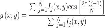1

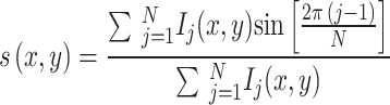2

The phasor plot is a 2D histogram of all the values g and s, corresponding to the pixels of the image. Background pixels are excluded from the phasor plot by setting an intensity threshold. A smoothing step is applied to g(x, y) and s(x, y) images using a 3 × 3 nearest neighbors weighted average filter.

The phasor plot shows the following two types of dotted reference lines: (i) phasor trajectories corresponding to Gaussian spectra of fixed bandwidth (FWHM = 10 nm and FWHM = 100 nm) and center wavelength varying from λ₁ to λ₄ in steps of 5 nm; (ii) phasor trajectories corresponding to Gaussian spectra of fixed center wavelength (λ₁, λ₂, λ₃, λ₄) and bandwidth varying from FWHM = 0 to FWHM = 400 nm in steps of 20 nm.

The phase of the phasor at each pixel is calculated as:

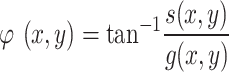3

With values between 0 and 2π. The phase wavelength image is calculated as:

4

So that φ = 0 correspond to λ_φ = λ₁ and φ = 2π(1–1/N) correspond to λ_φ = λ_N. In the specific case N = 4 the phase wavelength image is:

5

and the phase values φ = 0, π/2, π, 3/2 π correspond to the phase wavelengths λ₁, λ₂, λ₃, λ₄.

For the analysis shown in Fig. 3e, regions of interests (ROI) corresponding to different subcellular regions were defined in ImageJ using the intensity and the phase wavelength image. The ROI were used to extract the average value of phase wavelength in each ROI.

Fig. 3.

4C-spectral phasor imaging of ACDAN in live cells. (a) Representative 4-channels image of ACDAN in HeLa cell and (b) corresponding average fluorescence intensity in the 4 channels covering the range between 410 and 610 nm. (c) spectral phasor plot: the elongated phasor plot indicates the presence of multiple spectral signatures, corresponding to ACDAN emission in different cellular environments. (d) Intensity image obtained as the sum of the intensity in the 4 channels (top) and phase wavelength image (bottom). (e) Analysis of phase wavelength for different subcellular structures. Phase wavelengths values range from 490 to 510 nm. The analyzed subcellular regions are: nuclei, nuclear invaginations, vesicles identified for their bright intensity, cytoplasm, plasma membrane, vesicles identified as ‘blue’ in the phase wavelength image. Data represent mean ± s.d. of at least 10 different ROI.

The linear decomposition of the intensity into 2 components is done by expressing the phasor P(x, y) as the combination of two phasors P₁ and P₂²⁹. The phasors P₁ and P₂ can be selected by clicking directly on the phasor plot or calculated as corresponding to specific image regions. The fraction of intensity associated to component 1 is calculated as:

6

To limit values of fraction to values included between 0 and 1, the values of are filtered through a non-linear, logistic function of the form: , with , as described previously²⁹. The value of f₂ is calculated as: . Then the image corresponding to component k is calculated as:

7

i.e. is obtained by multiplying the fraction and the sum of the stack.

Results

Spectral phasor imaging using 4 channels of a commercial laser scanning microscope

The method’s scheme is reported in Fig. 1a–d. The images are acquired in a Leica SP8 confocal microscope using 4 contiguous, non-overlapping spectral detection bands. The 4 spectral windows sample pixel-to-pixel variations of emission spectra. The data are analyzed using the spectral phasor approach, which yields a phasor in the (g, s) plane for each pixel. Pixel-to-pixel variations of emission spectra are detected as shifts in the position of the phasors. The value of phase at each pixel (angular coordinate of the phasor) is converted into a value of wavelength to generate a phase wavelength image.

Fig. 1.

Spectral phasor using 4 channels of a commercial laser scanning microscope. (a–d) Schematic of the 4 C-spectral phasor method: (a) 4-color images are acquired using a commercial laser scanning microscope; (b) Emission spectra variations are sampled across four spectral detection windows; (c) For each pixel, a phasor in the (g, s) plane is computed, where phasor position shifts reflect pixel-to-pixel emission spectra variations; (d) a phase wavelength image () is calculated converting the value of phase into a value of wavelength. (e–g) Simulated data used for reference line generation. The spectral bandwidth of each detection channel is set to 50 nm. (e, top) Simulated Gaussian spectra with a narrow bandwidth (FWHM = 10 nm) and peak wavelength increasing from the value λ₁ (indicated by the arrow) in steps of 5 nm. (e, middle) Phasor plot of the simulated spectra. The red values (λ₁, λ₂, λ₃, λ₄) represent the center wavelengths of the 4 detection windows. Each red dot corresponds to a single spectrum. The narrow spectra are not uniformly sampled by the spectral windows, producing the polygonal trajectory. (e, bottom) Plot showing the phase value of the phasor versus the simulated peak wavelength for the 4C- and for the full spectral phasor. (f, top) Simulated Gaussian spectra with a broader bandwidth (FWHM = 100 nm) and peak wavelength increasing from the value λ₁ (indicated by the arrow) in steps of 5 nm. (f, middle) Phasor plot of the simulated spectra. Each red dot corresponds to a single spectrum. The broad spectra are more uniformly sampled, resulting in a curved trajectory, where each dot represents a 5 nm shift in peak wavelength. (f, bottom) Plot showing the phase value of the phasor versus the simulated peak wavelength for the 4C- and for the full spectral phasor. (g, top) Simulated Gaussian spectra of fixed center wavelengths (λ₁, λ₂, λ₃, λ₄) and bandwidths increasing from 0 to the value 400 nm in steps of 20 nm. (g, middle) Phasor plot of the simulated spectra. Each red dot corresponds to a single spectrum. These simulated spectra produce radial-like phasor trajectories.

Simulated data are useful to highlight the effect of using only 4 spectral windows on the spectral phasor plot²⁵ and to draw visual reference lines (Fig. 1e–g). In these simulations, we calculated how emission spectra of Gaussian shape and varying peak wavelength and bandwidth would be detected by 4 contiguous spectral windows and then calculated the corresponding position in the 4 C-spectral phasor. Each red dot corresponds to a single spectrum. The spectral bandwidth of each detection channel is set to be 50 nm. Gaussian spectra of narrow bandwidth (FWHM = 10 nm) and peak wavelength increasing in 5-nm steps are not uniformly sampled by the spectral windows and produce the polygonal trajectory shown in Fig. 1e (middle). Compared to the full spectral phasor (calculated using a large number of spectral channels, 150 in these simulations), the phase value increases stepwise versus the peak wavelength (Fig. 1e, bottom). This shows that the 4 C-spectral phasor is not sensitive to spectral shifts when the width of the spectra is narrower than the detection bandwidth. In contrast, Gaussian spectra of larger bandwidth (FWHM = 100 nm) are more uniformly sampled by the spectral windows and produce the curved trajectory shown in Fig. 1f (middle), where each dot represents a shift of 5 nm of the peak-wavelength. In this case, the phase value increases monotonically as a function of the simulated peak wavelength, similarly to the full spectral phasor (Fig. 1f, bottom). This shows that the 4 C-spectral phasor is sensitive to spectral shifts when the width of the spectra is larger than the detection bandwidth. Gaussian spectra of fixed center wavelength (λ₁, λ₂, λ₃, λ₄) and bandwidth varying from 0 to 400 nm in steps of 20 nm, produce radial-like phasor trajectories (Fig. 1g, middle). These radial-like trajectories are deformed when the peak wavelength is λ₁ or λ₄ because part of the emission spectrum falls outside the detection windows.

As a preliminary step, we performed spectral imaging of 2 fluorophores in solution: ANS in a water solution containing BSA (ANS-BSA, expected emission peak ~ 480 nm, expected FWHM ~ 90 nm) (Fig. 2a,b) and Rhodamine 110 in water (R110, expected emission peak ~ 520 nm, expected FWHM ~ 40 nm) (Fig. 2c,d). The data shows that the phasors of ANS-BSA and R110 are located at different angular positions in the phasor plot (mean phase wavelengths values λ_φ(ANS-BSA) = 505 nm and λ_φ(R110) = 543 nm), as expected. The different radial position (or, equivalently, different modulation value) is due to the different emission spectrum width of the two fluorophores. Linear combinations of the two dataset (indicated as ‘linear mixing’) produce phasors located along the straight line connecting the phasors of the pure species, confirming that the well-known linear combinations properties of the phasor³⁰ are preserved even though the reference trajectories are deformed towards the borders of the spectral range (Fig. 2e).

Fig. 2.

4-channels spectral imaging of fluorophores in solution. (a) Representative spectral imaging data of ANS in a water solution containing BSA and (b) corresponding average fluorescence intensity in the 4 channels. (c) Representative spectral imaging data of Rhodamine 110 in water and (d) corresponding average fluorescence intensity in the 4 channels. (e) The phasor plot showing different angular position for ANS-BSA and R110. The red values (435, 485, 535, 585) represent the center wavelengths of the 4 detection windows in nm. Linear combinations of the two datasets (‘linear mixing’) result in phasors positioned along the straight line connecting the phasors of the pure species. (f) The precision of the phase wavelength value, determined as the standard deviation of λ_φ across all pixels in the image for the ANS-BSA sample, plotted as a function of photon counts in the channel with maximum intensity. The red dashed line is a fit of the data to the equation Y = A (N_counts)^B, which yields B = − 0.50 and A = 20 nm.

The noise contained in the experimental data is propagated into the noise in the coordinates g and s of the phasor¹¹. The precision in the value of phase wavelength, determined as the standard deviation of the λ_φ values in all the pixels of the image, is reported on Fig. 2f for the sample of ANS-BSA, as a function of the photon counts in the channel of maximum intensity. As expected for Poisson or shot noise, the error scales as the inverse square root of the number of photon counts N_counts, σ = σ₀ (N_counts)^−1/2 (Fig. 2f), where σ₀ is a constant that represents the error on the phase wavelength when the number of photon counts is 1. In the conditions of the experiment, σ₀ = 20 nm, so that the value of the error σ is in the order of ~ 1 nm when the photon counts per pixel are ~ 300 (Fig. 2f).

Spectral imaging of the environment-sensitive probe ACDAN in live cells

Next, to demonstrate the applicability of the method, we performed spectral imaging of the environment-sensitive probe ACDAN in live HeLa cells. ACDAN is a member of the so-called DAN probes, a group of solvatochromic dyes developed to study macromolecular organizations of different kinds. Due to the methylene group substitution at the carbonyl group, this probe is soluble in water. It has been used as a molecular marker for studying crowding in vitro and in vivo^15,31–34. ACDAN spectrum shifts to green due to changes in environmental dielectric properties and the occurrence of dipolar relaxation. Inside cells, the responsible molecule for producing dipolar relaxation is water. ACDAN can sense the dipolar relaxation of a few water molecules around its moieties, and the energy lost during relaxation is reflected by lifetime and spectral changes.

A representative dataset is reported on Fig. 3a. ACDAN is excited at 405 nm, and the emission is detected in 4 channels covering the range between 410 and 610 nm (Fig. 3b). The average signal in the channel of maximum intensity (~ 150 a.u.) corresponds to an equivalent number of photon counts in the order of 280. The phasor plot is elongated (Fig. 3c), indicating the presence in the image of different spectral signatures corresponding to the emission of ACDAN in different environments. We identify several subcellular regions, with phase wavelengths ranging from 490 to 510 nm (Fig. 3d,e). A type of vesicles (identifiable as ‘blue’ in the phase wavelength image) has the most blue-shifted spectrum. These vesicles are probably lipid-containing vesicles, corresponding to the non-relaxed emission of ACDAN. The plasma membrane (identifiable as green color in the phase wavelength image) corresponds to about 495 nm. Then we identify cytoplasmic regions and nuclear invaginations at about 505 nm. This spectral region also includes vesicles identified as ‘bright’ in the intensity image. The brightness of these vesicles might be due to a higher ACDAN quantum yield or a higher ACDAN concentration. Finally, the nucleus is characterized by the lowest intensity and the most red-shifted spectrum, with a phase wavelength of about 510 nm.

Spectral imaging of the environment-sensitive probe nile red in live cells and organoids

Then, we performed spectral imaging of another environment-sensitive fluorophore, Nile Red. Nile Red is a hydrophobic dye that exhibits changes in its fluorescence based on the lipid content in its local environment, rather than directly binding to the lipids themselves. It is highly solvatochromic, meaning its emitted fluorescent light wavelength varies depending on the solvent, especially its polarity^35,36. As a result, this dye can be used as an indicator of local polarity, such as on the surface of nanoparticles³⁷. Nile Red is rapidly internalized from the plasma membrane of live cells and label also the cellular interior. Recently, variants of Nile Red have been developed for different applications^38,39.

First, we performed spectral imaging of Nile Red in live HeLa cells. A representative dataset is reported on Fig. 4a,b. Nile Red is excited at 488 nm and the emission was detected in 4 channels covering the spectral range between 525 and 725 nm. The average signal in the channel of maximum intensity (~ 160 a.u.) corresponds to an equivalent number of photon counts in the order of 300. We find similar and distinctive features with respect to ACDAN. The phasor is clearly elongated (Fig. 4c), indicating the presence of pixel-to-pixel spectral variations in the image¹⁷. Also in this case, we recognize the internal membrane, the plasma membrane, and the nucleus, as regions of increasing spectral red shift. However, in the case of Nile Red, the strongest signal comes from lipid vesicles which exhibit also the most blue-shifted spectral emission. Indeed, Nile Red is often used as a marker of lipid droplets^40,41. The spectral variations can be exploited to decompose the fluorescence signal of Nile Red into 2 components, indicated here as Nile Red 1 (corresponding to the less relaxed spectral emission) and Nile Red 2 (corresponding to the more relaxed spectral emission). Combined with Hoechst (which is excited at the different wavelength of 405 nm), this provides 3 color imaging with only 2 dyes (Fig. 4d).

Fig. 4.

4C-spectral phasor imaging of Nile Red in live cells and live intestinal organoids. (a) Intensity image of Nile Red in live HeLa cells. Scale bar 10 μm. (b) Phase wavelength image of Nile Red in live HeLa cells. (c) The elongated phasor plot reveals pixel-to-pixel spectral variations, distinguishing the internal membrane, the plasma membrane, and the nucleus as regions of increasing spectral redshift. (d) Spectral variations allow the decomposition of the fluorescence signal into two components: Nile Red 1, corresponding to the less relaxed spectral emission, and Nile Red 2, corresponding to the more relaxed spectral emission. Combined with Hoechst staining, this approach enables three-color imaging using only two dyes. (e) Intensity image of a live organoid labeled with Nile Red. Scale bar 20 μm. (f) Phase wavelength image of a live organoid labeled with Nile Red. (g) Decomposition of Nile Red in 2 components provides a 3-color image, with Hoechst in one channel, lipid vesicles in another channel and internal membranes in the other. Scale bar 20 μm. In the zoom-in, scale bar is 5 μm. (h) 3-color imaging performed on the same type of organoids using a commercial labeling reagent (ORGANELLE-ID-RGB), which contains a mixture of 3 dyes targeting nuclei, mitochondria, and lysosomes. Scale bar 20 μm. In the zoom-in, scale bar is 5 μm. (i) Average fluorescence intensity as a function of the 4 channels covering the spectral range between 525 and 725 nm, for the sample of Nile Red in HeLa cells. (j) Average fluorescence intensity as a function of the 4 channels covering the spectral range between 525 and 725 nm, for the sample of Nile Red in organoids.

As an example of application in a more complex system, we tested the same experimental approach on live intestinal organoids (Fig. 4e–h). Intestinal organoid models are raising increasing interest due to their superior ability to mimic cell-type composition and complex tissue organization in vitro^27,42–45compared to more conventional intestinal cell lines such as CaCo-2⁴⁶. An example of organoid labeled with Nile Red is reported on Fig. 4e,f. The 4 C-spectral phasor analysis has a similar pattern observed in live cells. Also in this case, decomposition in 2 components provides a 2-color image with the lipid vesicles in one channel and internal membranes in the other. In combination with Hoechst this approach provides 3 color imaging with only 2 dyes (Fig. 4g). For comparison, we performed 3 color imaging of the same type of organoids using a commercial labeling reagent containing a mixture of 3 dyes (ORGANELLE-ID-RGB) targeting nuclei, mitochondria and lysosomes (Fig. 4h).

Spectral unmixing of green and yellow fluorescent proteins

To demonstrate applicability of the method to spectral unmixing of fluorescent proteins, we performed 4-channel imaging of HEK293T cells expressing mEmerald-actin and YFP-CAAX, where CAAX is a peptide motif for prenylation and subsequent targeting to the inner leaflet of the plasma membrane⁴⁷. Compared to ACDAN or Nile Red, the emission spectra of the proteins are narrower, and the Stokes shift smaller. The two fluorescent proteins are excited at 488 nm and their emission was detected in 4 channels covering the range between 495 and 615 nm, with a spectral detection window of 30 nm for each channel.

The phasors corresponding to cells expressing only one of the two proteins are shown in Fig. 5a,b. The average phase wavelength corresponding to mEmerald-actin (515 nm) is shifted of about ~ 15 nm with respect to the average phase wavelength corresponding to EYFP-CAAX (527 nm), in keeping with an expected peak shift of ~ 20 nm. The phasor corresponding to cells co-transfected with mEmerald-actin and EYFP-CAAX is shown in Fig. 5c. The phasor is clearly elongated, in keeping with the presence of two different fluorescent species in the image, and located along the line connecting the phasors of the pure species. The phase wavelength image allows identifying cells with different spectral fingerprints: for instance a cell with predominant expression of EYFP-CAAX (indicated by a star) or a cell with predominant expression of mEmerald-actin (indicated by an arrowhead) (Fig. 5e). Phasor decomposition provides spectrally unmixed images corresponding to the two fluorescent proteins (Fig. 5f).

Fig. 5.

4C-spectral phasor unmixing of green and yellow fluorescent proteins expressed in HEK293T cells. (a) 4-channel imaging of HEK293T cells expressing only mEmerald-actin and corresponding phasor plot. (b) 4-channel imaging of HEK293T cells expressing only EYFP-tagged CAAX (EYFP-CAAX) and corresponding phasor plot. (c)  4-channel imaging of HEK293T cells co-expressing mEmerald-actin and EYFP-tagged CAAX (EYFP-CAAX) and corresponding phasor plot. The elongated phasor plot reflects the presence of two distinct fluorescent species in the image. (d)  Emission detected in 4 channels covering the range between 495 and 615 nm, with a spectral detection window of 30 nm for each channel. (e) The phase wavelength image reveals cells with different spectral fingerprints, such as a cell predominantly expressing EYFP-CAAX (indicated by a star) or a cell predominantly expressing mEmerald-actin (indicated by an arrowhead). (f) Phasor decomposition provides spectrally unmixed images corresponding to the two fluorescent proteins.

We note that similar results could also be obtained using other linear unmixing algorithms². Here, we have focused on the generation of the spectral phasor which provides an unbiased visualization of spectral imaging data in the phasor plot. The phasor plot visualization is useful to interpret the spectral information content in the spectral image prior to any other type of analysis.

Discussion

We have demonstrated that spectral analysis can be performed on a commercial laser scanning microscope not equipped with a spectral detector, just using simultaneous acquisition in 4 different detector channels and spectral phasor analysis. There are 3 main advantages in the proposed approach. First of all, it is compatible with any confocal microscope equipped with 4 detectors. In particular, we have exploited the capability of the Leica detection system to change almost freely the spectral detection bands of the 4 channels in such a way to sample the emission spectra of the fluorophores. Indeed, we have used 50 nm bands for ACDAN and Nile Red and 30 nm for the fluorescent proteins mEmerald and EYFP. The second important point is that the temporal resolution of this approach is the same of the confocal microscope, since the 4 channels are recorded simultaneously. This makes the method a powerful alternative to the relatively slow lambda scan mode, especially for live cell imaging applications. Finally, the method is more photon-effective compared to the lambda scan mode, since photons from all parts of the emission spectrum are detected and not wasted. In contrast, as shown by the simulated data in Fig. 1, the 4C-spectral phasor is not sensitive if the width of the spectra is narrower than the detection bandwidth and/or if the spectra are peaked at the border of the detection range.

In terms of representative applications, we have demonstrated that the 4 C-spectral phasor method can be used in live samples stained with environment-sensitive dyes and is able detect spectral shifts of few nanometers between different subcellular regions. Labeling with environment-sensitive dyes can be useful to map the biophysical and biochemical properties of cell environment, or simply to identify multiple subcellular targets with the use of a lower number of dyes. As another representative application, we have demonstrated unmixing of fluorescent proteins with spectra overlapping in the green-yellow region of the visible spectrum. We have tested the method on 2 different commercial microscopes: Leica SP8 and Leica STELLARIS8. In particular, in the Leica SP8 setup we had to use different types of detectors (i.e. photomultiplier and hybrid), so we have adjusted the gain to get approximately the same yield in the four channels.

In summary, we described a method to perform spectral analysis in commercial microscopes that are not equipped with a spectral detector. The method can be used to perform fast spectral analysis in solutions, live cells and live organoids. This tool will increase the portfolio of advanced fluorescence spectroscopy methods that can be performed on commercial microscopes, thanks to dedicated software^48–52. We believe that this new tool will be useful to researchers having access to commercial confocal microscopes and will foster the use of advanced fluorescence spectroscopy methods in their applications.

Author contributions

L.L., M.G. and L.M. designed the study. A.P., E.L., A.A., A.C., S.S. prepared samples. L.L., E.L., A.A., A.C., P.B. collected data. L.L. wrote software. E.L., P.B. and L.L. performed data analysis. All authors analyzed and discussed results. L.L., E.L., L.M., A.C., A.A. wrote manuscript. All authors critically reviewed the manuscript.

Data availability

Data sets generated during the current study are available from the corresponding author on reasonable request.

Declarations

Competing interests

The authors declare no competing interests.

Software availability

A user-friendly, stand-alone version of the 4 C-spectral phasor software generated in Matlab is available at https://github.com/llanzano/4CSpectralPhasor.

References

- 1.Garini, Y., Young, I. T. & McNamara, G. Spectral imaging: principles and applications. Cytometry Part. A. 69A, 735–747 (2006). [DOI] [PubMed] [Google Scholar]
- 2.Zimmermann, T., Rietdorf, J. & Pepperkok, R. Spectral imaging and its applications in live cell microscopy. FEBS Lett.546, 87–92 (2003). [DOI] [PubMed] [Google Scholar]
- 3.Sezgin, E., Waithe, D., Bernardino de la Serna, J. & Eggeling, C. Spectral imaging to measure heterogeneity in membrane lipid packing. ChemPhysChem16, 1387–1394 (2015). [DOI] [PMC free article] [PubMed] [Google Scholar]
- 4.Gao, L. & Smith, R. T. Optical hyperspectral imaging in microscopy and spectroscopy—a review of data acquisition. J. Biophoton. 8, 441–456 (2015). [DOI] [PMC free article] [PubMed] [Google Scholar]
- 5.Mukherjee, T. et al. Live-cell imaging of the nucleolus and mapping mitochondrial viscosity with a dual function fluorescent probe. Org. Biomol. Chem.19, 3389–3395 (2021). [DOI] [PubMed] [Google Scholar]
- 6.Tosto, R. et al. A spectroscopic study on the amyloid-β interaction with clicked peptide‐porphyrin conjugates: a vision toward the detection of Aβ peptides in aqueous solution. ChemBioChem. 25, (2024). [DOI] [PMC free article] [PubMed]
- 7.Zucker, R. M., Rigby, P., Clements, I., Salmon, W. & Chua, M. Reliability of confocal microscopy spectral imaging systems: use of multispectral beads. Cytometry Part. A. 71A, 174–189 (2007). [DOI] [PubMed] [Google Scholar]
- 8.Haraguchi, T., Shimi, T., Koujin, T., Hashiguchi, N. & Hiraoka, Y. Spectral imaging fluorescence microscopy. Genes Cells. 7, 881–887 (2002). [DOI] [PubMed] [Google Scholar]
- 9.Lochocki, B. et al. Multimodal, label-free fluorescence and Raman imaging of amyloid deposits in snap-frozen alzheimer’s disease human brain tissue. Commun. Biol.4, 474 (2021). [DOI] [PMC free article] [PubMed] [Google Scholar]
- 10.Meleppat, R. K. et al. In situ morphologic and spectral characterization of retinal pigment epithelium organelles in mice using multicolor confocal fluorescence imaging. Investig. Opthalmol. Visual Sci.61, 1 (2020). [DOI] [PMC free article] [PubMed] [Google Scholar]
- 11.Clayton, A. H. A., Hanley, Q. S. & Verveer, P. J. Graphical representation and multicomponent analysis of single-frequency fluorescence lifetime imaging microscopy data. J. Microsc. 213, 1–5 (2004). [DOI] [PubMed] [Google Scholar]
- 12.Digman, M. A., Caiolfa, V. R., Zamai, M. & Gratton, E. The phasor approach to fluorescence lifetime imaging analysis. Biophys. J.94, L14–L16 (2008). [DOI] [PMC free article] [PubMed] [Google Scholar]
- 13.Cutrale, F. et al. Hyperspectral phasor analysis enables multiplexed 5D in vivo imaging. Nat. Methods. 14, 149–152 (2017). [DOI] [PubMed] [Google Scholar]
- 14.Ranjit, S., Malacrida, L., Jameson, D. M. & Gratton, E. Fit-free analysis of fluorescence lifetime imaging data using the phasor approach. Nat. Protoc.13, 1979–2004 (2018). [DOI] [PubMed] [Google Scholar]
- 15.Vorontsova, I. et al. In vivo macromolecular crowding is differentially modulated by Aquaporin 0 in zebrafish lens: insights from a nanoenvironment sensor and spectral imaging. Sci Adv8, (2022). [DOI] [PMC free article] [PubMed]
- 16.Hedde, P. N., Cinco, R., Malacrida, L., Kamaid, A. & Gratton, E. Phasor-based hyperspectral snapshot microscopy allows fast imaging of live, three-dimensional tissues for biomedical applications. Commun. Biol.4, 721 (2021). [DOI] [PMC free article] [PubMed] [Google Scholar]
- 17.Bianchetti, G., Di Giacinto, F., De Spirito, M. & Maulucci, G. Machine-learning assisted confocal imaging of intracellular sites of triglycerides and cholesteryl esters formation and storage. Anal. Chim. Acta. 1121, 57–66 (2020). [DOI] [PubMed] [Google Scholar]
- 18.Fu, D. & Xie, X. S. Reliable cell segmentation based on spectral phasor analysis of hyperspectral stimulated Raman scattering imaging data. Anal. Chem.86, 4115–4119 (2014). [DOI] [PubMed] [Google Scholar]
- 19.Yao, Z. et al. Multiplexed bioluminescence microscopy via phasor analysis. Nat. Methods. 19, 893–898 (2022). [DOI] [PubMed] [Google Scholar]
- 20.Malacrida, L. et al. Spectral phasor analysis of LAURDAN fluorescence in live A549 lung cells to study the hydration and time evolution of intracellular lamellar body-like structures. Biochim. Et Biophys. Acta (BBA) Biomembr.1858, 2625–2635 (2016). [DOI] [PMC free article] [PubMed] [Google Scholar]
- 21.Lanzanò, L. et al. Encoding and decoding spatio-temporal information for super-resolution microscopy. Nat. Commun.6, 6701 (2015). [DOI] [PMC free article] [PubMed] [Google Scholar]
- 22.Sarmento, M. J. et al. Exploiting the tunability of stimulated emission depletion microscopy for super-resolution imaging of nuclear structures. Nat. Commun.9, 3415 (2018). [DOI] [PMC free article] [PubMed] [Google Scholar]
- 23.Cainero, I. et al. Chromatin investigation in the nucleus using a phasor approach to structured illumination microscopy. Biophys. J.120, 2566–2576 (2021). [DOI] [PMC free article] [PubMed] [Google Scholar]
- 24.D’Amico, M. et al. A phasor-based approach to improve optical sectioning in any confocal microscope with a tunable pinhole. Microsc. Res. Tech.85, 3207–3216 (2022). [DOI] [PMC free article] [PubMed] [Google Scholar]
- 25.Fereidouni, F., Bader, A. N. & Gerritsen, H. C. Spectral phasor analysis allows rapid and reliable unmixing of fluorescence microscopy spectral images. Opt. Express. 20, 12729 (2012). [DOI] [PubMed] [Google Scholar]
- 26.Andrews, L. M., Jones, M. R., Digman, M. A. & Gratton, E. Spectral phasor analysis of pyronin Y labeled RNA microenvironments in living cells. Biomed. Opt. Express. 4, 171 (2013). [DOI] [PMC free article] [PubMed] [Google Scholar]
- 27.Sato, T. et al. Long-term expansion of epithelial organoids from human colon, adenoma, adenocarcinoma, and barrett’s epithelium. Gastroenterology141, 1762–1772 (2011). [DOI] [PubMed] [Google Scholar]
- 28.Pelicci, S., Tortarolo, G., Vicidomini, G., Diaspro, A. & Lanzanò, L. Improving SPLIT-STED super-resolution imaging with tunable depletion and excitation power. J. Phys. D Appl. Phys.53, 234003 (2020). [Google Scholar]
- 29.Cainero, I. et al. Measuring nanoscale distances by structured illumination microscopy and image Cross-Correlation spectroscopy (SIM-ICCS). Sensors21, 2010 (2021). [DOI] [PMC free article] [PubMed] [Google Scholar]
- 30.Torrado, B., Malacrida, L. & Ranjit, S. Linear combination properties of the phasor space in fluorescence imaging. Sensors22, 999 (2022). [DOI] [PMC free article] [PubMed] [Google Scholar]
- 31.Mangiarotti, A. et al. Biomolecular condensates modulate membrane lipid packing and hydration. Nat. Commun.14, 6081 (2023). [DOI] [PMC free article] [PubMed] [Google Scholar]
- 32.Otaiza-González, S. et al. The innards of the cell: studies of water dipolar relaxation using the ACDAN fluorescent probe. Methods Appl. Fluoresc. 10, 044010 (2022). [DOI] [PubMed] [Google Scholar]
- 33.Thoke, H. S., Thorsteinsson, S., Stock, R. P., Bagatolli, L. A. & Olsen, L. F. The dynamics of intracellular water constrains glycolytic oscillations in Saccharomyces cerevisiae. Sci. Rep.7, 16250 (2017). [DOI] [PMC free article] [PubMed] [Google Scholar]
- 34.Begarani, F. et al. Capturing Metabolism-Dependent solvent dynamics in the lumen of a trafficking lysosome. ACS Nano. 10.1021/acsnano.8b07682 (2019). [DOI] [PubMed]
- 35.Demchenko, A. P., Mély, Y., Duportail, G. & Klymchenko, A. S. Monitoring biophysical properties of lipid membranes by environment-sensitive fluorescent probes. Biophys. J.96, 3461–3470 (2009). [DOI] [PMC free article] [PubMed] [Google Scholar]
- 36.Mukherjee, S., Raghuraman, H. & Chattopadhyay, A. Membrane localization and dynamics of nile red: effect of cholesterol. Biochim. Et Biophys. Acta (BBA) Biomembr.1768, 59–66 (2007). [DOI] [PubMed] [Google Scholar]
- 37.Boumelhem, B. B. et al. Intracellular flow cytometric lipid analysis—a multiparametric system to assess distinct lipid classes in live cells. J. Cell. Sci135, (2022). [DOI] [PubMed]
- 38.Danylchuk, D. I., Moon, S., Xu, K. & Klymchenko, A. S. Switchable solvatochromic probes for Live-Cell Super‐resolution imaging of plasma membrane organization. Angew. Chem.131, 15062–15066 (2019). [DOI] [PubMed] [Google Scholar]
- 39.Lauritsen, L. et al. Ratiometric fluorescence nanoscopy and lifetime imaging of novel nile red analogs for analysis of membrane packing in living cells. Sci. Rep.14, 13748 (2024). [DOI] [PMC free article] [PubMed] [Google Scholar]
- 40.Greenspan, P., Mayer, E. P. & Fowler, S. D. Nile red: a selective fluorescent stain for intracellular lipid droplets. J. Cell. Biol.100, 965–973 (1985). [DOI] [PMC free article] [PubMed] [Google Scholar]
- 41.Diaz, G., Melis, M., Batetta, B., Angius, F. & Falchi, A. M. Hydrophobic characterization of intracellular lipids in situ by nile red red/yellow emission ratio. Micron39, 819–824 (2008). [DOI] [PubMed] [Google Scholar]
- 42.Nikolaev, M. et al. Homeostatic mini-intestines through scaffold-guided organoid morphogenesis. Nature585, 574–578 (2020). [DOI] [PubMed] [Google Scholar]
- 43.Fujii, M. et al. Human intestinal organoids maintain self-renewal capacity and cellular diversity in niche-inspired culture condition. Cell. Stem Cell.23, 787–793e6 (2018). [DOI] [PubMed] [Google Scholar]
- 44.Almeqdadi, M., Mana, M. D., Roper, J. & Yilmaz, Ö. H. Gut organoids: mini-tissues in culture to study intestinal physiology and disease. Am. J. Physiol.-Cell Physiol.317, C405–C419 (2019). [DOI] [PMC free article] [PubMed] [Google Scholar]
- 45.Liberali, P. & Schier, A. F. The evolution of developmental biology through conceptual and technological revolutions. Cell187, 3461–3495 (2024). [DOI] [PubMed] [Google Scholar]
- 46.Giral, H. et al. NHE3 regulatory factor 1 (NHERF1) modulates intestinal Sodium-dependent phosphate transporter (NaPi-2b) expression in apical microvilli. J. Biol. Chem.287, 35047–35056 (2012). [DOI] [PMC free article] [PubMed] [Google Scholar]
- 47.Clarke, S. Protein isoprenylation and methylation at carboxyl-terminal cysteine residues. Annu. Rev. Biochem.61, 355–386 (1992). [DOI] [PubMed]
- 48.BRown, C. M. et al. Raster image correlation spectroscopy (RICS) for measuring fast protein dynamics and concentrations with a commercial laser scanning confocal microscope. J. Microsc. 229, 78–91 (2008). [DOI] [PMC free article] [PubMed] [Google Scholar]
- 49.Dalal, R. B., Digman, M. A., Horwitz, A. F., Vetri, V. & Gratton, E. Determination of particle number and brightness using a laser scanning confocal microscope operating in the analog mode. Microsc. Res. Tech.71, 69–81 (2008). [DOI] [PubMed] [Google Scholar]
- 50.Moens, P. D. J., Gratton, E. & Salvemini, I. L. Fluorescence correlation spectroscopy, raster image correlation spectroscopy, and number and brightness on a commercial confocal laser scanning microscope with analog detectors (Nikon C1). Microsc. Res. Tech.74, 377–388 (2011). [DOI] [PMC free article] [PubMed] [Google Scholar]
- 51.Hendrix, J., Dekens, T., Schrimpf, W. & Lamb, D. C. Arbitrary-region raster image correlation spectroscopy. Biophys. J.111, 1785–1796 (2016). [DOI] [PMC free article] [PubMed] [Google Scholar]
- 52.Longo, E., Scalisi, S. & Lanzanò, L. Segmented fluorescence correlation spectroscopy (FCS) on a commercial laser scanning microscope. Sci. Rep.14, 17555 (2024). [DOI] [PMC free article] [PubMed] [Google Scholar]
Associated Data
This section collects any data citations, data availability statements, or supplementary materials included in this article.
Data Availability Statement