Deep-Learning to Map a Benchmark Dataset of Non-amputee Ambulation for Controlling an Open Source Bionic Leg

Abstract

Powered lower-limb prosthetic devices may be becoming a promising option for amputation patients. Although various methods have been proposed to produce gait trajectories similar to those of non-disabled individuals, implementing these control methods is still challenging. It remains unclear whether these methods provide appropriate, safe, and intuitive locomotion as intended. This paper proposes the direct mapping of the voluntary movement of a residual limb (i.e., thigh) to the desired impedance parameters for amputated limbs (i.e., knee and ankle). The proposed model was learned from the gait trajectories of intact limb individuals from a publicly available biomechanics dataset, and was applied to control the prosthetic leg without post-tuning the network. Thus, the proposed method does not require training time with individuals with amputation nor configuration time for its use, and it provides a closely resembling gait trajectory of the intact limb. For preliminary testing, three able-bodied subjects participated in bypass tests. The proposed model accomplished intuitive and reliable level-ground walking at three different step lengths: self-selected, long-, and short-step lengths. The results indicate that intact benchmark data with different sensor configurations can be directly used to train the model to control prosthetic legs.

I. Introduction

MILLIONS of people live with lower-limb amputation, and even when using state-of-the-art microprocessor-controlled passive prostheses, they have limited mobility and functional deficits [1], [2]. Bionic legs—devices that are powered and appropriately controlled—are a promising option to restore more function compared to passive prostheses, as they are capable of doing mechanical work and restoring a gait that more closely resembles that of intact limb individuals [3].

The control of bionic legs is commonly achieved using a three-level hierarchical controller. The high-level controller in-terprets human intentions and predicts the desired ambulation modes, such as level-ground walking or ascending/descending stairs. The mid-level controller generates the resulting gait trajectory parameters for the desired leg behavior. Finally, the low-level controller generates motor commands with feedback loops to control a specific parameter derived by the mid-level controller, such as position, velocity, torque, or impedance.

A variety of methods have been proposed to create mid-level controllers. For example, neuromuscular model control [4] mimics the underlying dynamics of the human neuromuscular system driven by virtual muscles. Phase-based control [5] parameterizes the gait cycle by a human-inspired phase variable, such as the thigh phase angle. Another common mid-level control approach uses an impedance-inspired controller where a number of impedance parameters are implemented within a finite-state machine. Using this approach, the parameters are carefully tuned, usually by hand. However, parameter tuning is a time-consuming and subjective process that relies on the experiences of therapists and prosthetists [6]. Thus, more recently, machine learning [7] and deep learning [8] techniques have been proposed for more intuitive and efficient tuning. Regardless of which mid-level control approach is used, implementation is still challenging, and it remains unclear which method works best or generalizes best across various activities. Individuals with amputation interact with their devices and the surrounding environment using their residual limbs, which are attached to the device through a socket. For example, individuals with unilateral transfemoral amputation (i.e., above-knee amputation) wear the socket on their thigh. They can voluntarily move their residual limb to change their thigh angle, making it a useful signal to help control the device (using the previously mentioned phase-based control approach as an example). The interaction between the user and environment can be sensed and contextualized by sensors (e.g., a load cell) and the current operational state of the device. For example, a load cell can measure the forces and moments created when the user shifts their weight onto or off the device by adjusting their intact hip joint and their non-amputated side. These voluntary control signals and resulting sensor recordings are powerful tools from which controllers can be created.

Deep neural networks (DNNs) are a rapidly evolving field of research and have been used in a variety of applications in the fields of the exoskeleton and prosthetic devices. DNNs are layered structures with various learnable parameters and have a powerful capability to learn non-linear input-output mappings. For example, convolutional neural networks and long short-term memory (LSTM) networks were used to estimate the human gait phase and used a generated hip torque to control a robotic hip exoskeleton [9]. Multi-stream LSTM dueling models have been used to predict the arm trajectory based on electromyography (EMG) data and inertial measurement unit data to control an upper limb exoskeleton [10]. Our research group has used DNNs to augment sensor data to learn robust representations of movement intention for powered leg prostheses [11] and improve classification performance in the presence of noise for EMG-based control of upper-limb prosthetic limbs [12].

In this paper, we propose DNN-based direct mapping between the voluntary movement of residual limbs and impedance parameters to generate the desired movement of the bionic leg. We trained the proposed model using data collected from a publicly available benchmark dataset measured from intact limb individuals. Then, the DNN model collected thigh angle and vertical load using the sensors available on the device and generated knee and ankle commands for a low-level controller in real-time. In terms of joint angle prediction, Gaussian process regression-based methods have been proposed. Thigh angle and angular velocity were used to predict knee angle [13]. Muscle activities were analyzed using EMG [14], ultrasound imaging [15], and their sensor fusion [16]. However, validation of the real-time control of prosthetics is yet to be performed.

The proposed method reduces the training time and configuration time required to use a prosthetic leg by eliminating the mid-level controller while providing impedance parameters for a gait trajectory closely resembling that of intact limb individuals. The proposed system was demonstrated to control powered knee and ankle with intact-limb subjects using a bypass adaptor. We hypothesized that the DNN could (i) find the relationship between voluntary movement (i.e., thigh angle and vertical load) and movement of joints that required control and (ii) generate a reliable and safe gait trajectory without post-tuning the system.

II. Methods

A. Open Source Benchmark Dataset

We used an open-source dataset of lower-limb biomechanics [17] to learn the gait trajectory of intact limb individuals. These data contain several mechanical sensor data and EMG data recorded from 22 intact limb subjects performing several ambulation modes, including stair ascent, ramp ascent, and level-ground walking. For this work, we used only data from walking on the treadmill, as we required data from continuous gait cycles with a ground reaction force to train the proposed system. The treadmill dataset contains data from walking at speeds that range from 0.5 to 1.85 m/s. From this dataset, we used the motion capture data (thigh (hip), knee, and ankle angles), the force plate data (vertical load), and five EMG data channel recordings (gluteus medius, vastus medialis, biceps femoris, gastrocnemius, and tibialis anterior).

B. Open Source Bionic Leg

The proposed method was evaluated using a self-contained open-source bionic leg (OSL). The OSL includes a powered knee and ankle, in which joints are actuated along the sagittal plane. The actuation at each joint is powered by brushless DC motors with a closed-loop controller (Dephy Inc., Cambridge, Mass.) powered by a 36 V lithium-polymer battery back. The knee uses a three-stage belt-drive transmission, and the ankle uses a two-stage belt-drive transmission in series with a single-stage kinematic linkage. The OSL also includes several sensors that can be used to monitor the state of the device. The OSL has a total mass of ∼4 kg. Additional details for the hardware, available sensors, and the built-in controller can be found in [18].

C. Control of the OSL

We used an impedance controller to generate torques for the knee and ankle based on the following equation:

$${\tau }_i=-k_i\left({\theta }_i-{\theta }_i^{eq}\right)-b{\dot{\theta }}_i$$ (1)

where i represents the knee or ankle joint, τ represents the joint torque, θ and $\dot{\theta }$ represent the joint angle and velocity, respectively, and k, b, and θ^eq denote the stiffness, damping coefficient, and equilibrium angle, respectively. The sign conventions for the knee joint angles were that knee flexion was positive and knee extension was negative. In the case of the ankle, dorsiflexion was positive, and plantar flexion was negative. The proposed DNN method generates these impedance parameters for the OSL knee and ankle by training the model using only the benchmark dataset.

D. DNN System

The proposed DNN system aims to predict the control parameters for the prosthetic legs from a benchmark dataset and then control the leg in real-time. In other words, the DNN system should collect sensor data from prosthetic legs and generate impedance parameters periodically at a fixed rate, without delaying or disturbing the routine functionalities of the prosthetic leg. We chose the vertical load and thigh angle as input data to map the powered knee and ankle impedance parameters. The vertical load provides information regarding two distinct phases: stance and swing. In addition, the thigh angle can be voluntarily and intuitively controlled by the residual limbs of individuals with transfemoral amputations. The benchmark dataset needs to be transformed to the OSL prior to mapping the desired impedance parameters using DNNs.

1). Data Conversion:

The benchmark dataset and the OSL use different sensor coordinate systems. For example, in the case of the benchmark dataset, knee flexion is a negative value as opposed to the OSL. Fig. 1 shows the exemplary benchmark data (AB10, part of treadmill_07_01) and its transformed data for the OSL. The vertical load (Fig. 1(a)) was divided by the user weight to normalize it (Fig. 1(b)). The directions of the thigh and knee angles were changed (Fig. 1(c)-Fig. 1(d)). The sensor value ranges for the knee and ankle were also adjusted (Fig. 1(d)) as follows:

$$\begin{gathered} {\theta }_{knee}=\max \left\{0,{\theta }_{knee}^{subject}-{\theta }_{knee}^{25}\right\} \\ {\theta }_{ankle}={\theta }_{ankle}^{subject}-{\theta }_{ankle}^{70} \end{gathered}$$ (2)

where ${\theta }_{knee}^{subject}$ and ${\theta }_{ankle}^{subject}$ represent the knee and ankle angles from each subject, respectively, and ${\theta }_i^n$ denotes the nth percentile of angles from all subjects. These percentile values were heuristically determined for the purposes of accommodating the alignment of the device when attached to the bypass prosthesis and matching the sensor ranges between the device and the benchmark dataset.

Fig. 1.

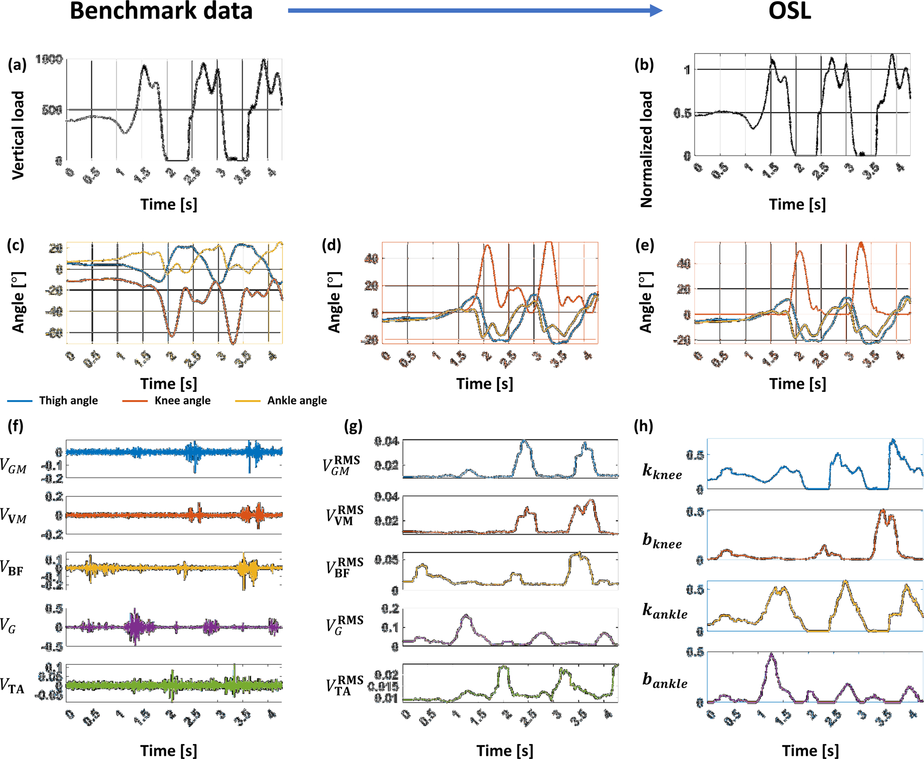
Conversion of the benchmark data to the OSL data through exemplary data (AB10, part of treadmill_07_01). The vertical load measured by force plate (a) was normalized by user weight (b). In the case of the joint angles (c), the direction of the thigh and knee angles was changed to compensate for the difference in the sensor coordinate system, and the bias was removed from the knee and ankle angles (d). In addition, we added a constraint for the knee to prevent knee flexion in mid-stance (e). In the case of the stiffness and damping coefficient, RMS envelopes (g) of five EMG data (f) were utilized to generate synthetic stiffness and damping coefficient (h).

The benchmark dataset includes stance-phase knee flexion up to 20 degrees, as shown in Fig. 1(d). In preliminary testing, this knee flexion in mid-stance felt uncomfortable to testers; thus, we added a constraint for the knee (Fig. 1(e)) as follows:

$${{\theta }^{\prime }}_{knee}={\theta }_{knee}\times {\left(1-F_z\right)}^2$$ (3)

where F_z denotes the normalized vertical load.

For the stiffness and damping coefficients, EMG data from five muscles (Fig. 1(f)) were used to generate synthetic stiffness and damping coefficients for the knee and ankle. The gluteus medius (V_GM ) contributes to walking stability during thigh abduction, vastus medialis (V_{V M} ) contributes to knee extension, biceps femoris (V_BF ) contributes to knee flexion, gastrocnemius (V_G) contributes to plantar flexion, and tibialis anterior (V_TA) contributes to dorsiflexion; these muscles provide the primary force driving the corresponding actions [19]. To generate the stiffness and damping coefficients, the root mean square (RMS) envelope of the EMG data is first extracted (Fig. 1(g)). The RMS envelope at time t represents the RMS value from t to t + 200 ms. Here, no method has been utilized to correct or remove artifacts from EMG data before the RMS envelope. Then, the synthetic stiffness and damping coefficient (Fig. 1(h)) were obtained as follows:

$$\begin{gathered} k_{knee}=F_z\left(V_{GM}^{RMS}+V_{VM}^{RMS}+V_{BF}^{RMS}\right) \\ {b}_{knee}=V_{VM}^{RMS}\times V_{BF}^{RMS} \\ {k}_{ankle}=F_z\left(V_{GM}^{RMS}+V_G^{RMS}+V_{TA}^{RMS}\right) \\ {b}_{ankle}=V_G^{RMS}\times V_{TA}^{RMS} \end{gathered}$$ (4)

where V^RMS represents RMS envelopes of the EMG data. Finally, the synthetic stiffness and damping coefficient were extracted, and their values were normalized and bounded between 0 and 1 as follows:

$${p^{\prime }}_i=\frac{p_i-p_i^5}{p_i^{95}-p_i^5}$$ (5)

where p_i and ${p^{\prime }}_i$ represent impedance parameter and its normalized value respectively, and $p_i^n$ represents nth percentile of the parameter from all subjects. This relationship between the EMG data and impedance parameters was heuristically determined. The details are provided in Discussion.

Fig. 2 displays the gait trajectories and corresponding impedance parameters that were ultimately extracted from the benchmark dataset.

Fig. 2.

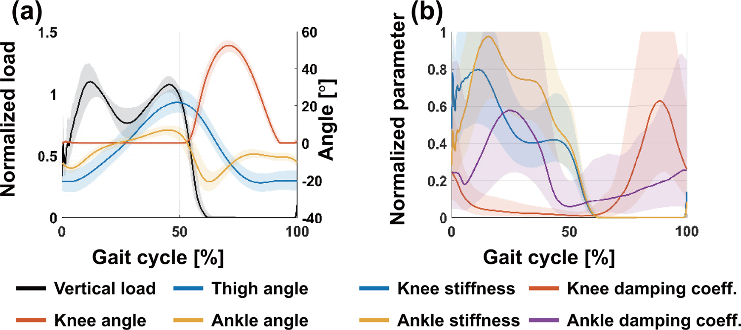
Gait trajectory (a) and corresponding stiffness and damping coefficient (b) were extracted from 22 non-disabled subjects. All plots show 75th and 25th percentiles in lighter bands.

The proposed system parsed sensor data every 5 ms (i.e., 200 Hz) from the OSL. For the benchmark dataset, the joint angles (i.e., motion capture data), the vertical load (i.e., force plate data), and the EMG data have a sampling frequency of 200 Hz, 1 kHz, and 1 kHz, respectively. Therefore, the vertical load and synthetic stiffness/damping coefficient were downsampled to 200 Hz to match sampling frequencies.

2). Network Configuration:

An overview of the proposed system architecture is presented in Fig. 3. Two independent networks were used to extract impedance parameters. The first DNN extracts the equilibrium angle for the knee and ankle (${\theta }_{knee}^{eq}$ and ${\theta }_{ankle}^{eq}$) from the vertical load and thigh angle (F_z and θ_thigh), and the second DNN extracts the stiffness (k_knee and k_ankle) and damping coefficient (b_knee and b_ankle) from the vertical load and thigh, knee, and ankle angles (F_z, θ_thigh, θ_knee, and θ_ankle).

Fig. 3.

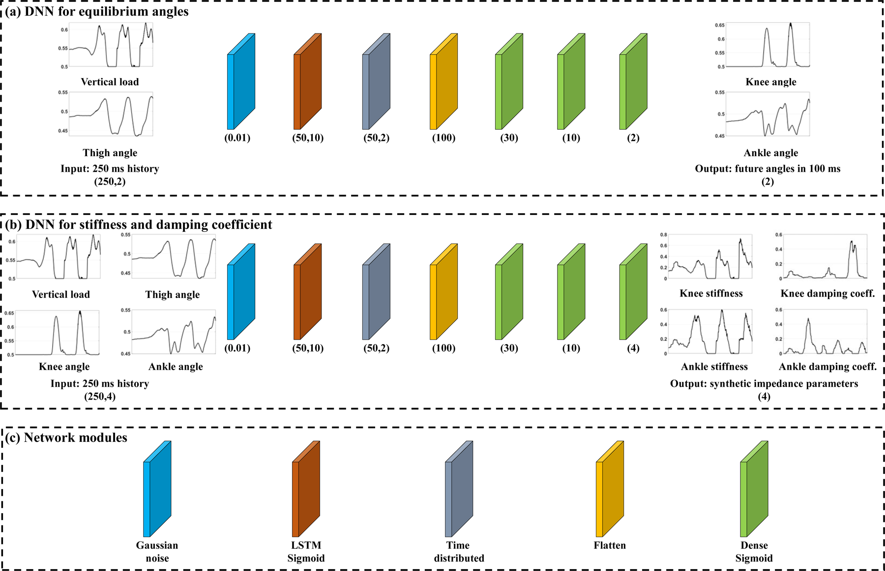
Architecture of the proposed system. In the case of the equilibrium angle (a), the model takes the history of the vertical load and thigh angle as the inputs. In the case of the stiffness and damping coefficient (b), the model takes the history of the vertical load, thigh, knee, and ankle angles. (c) The network modules represent the function of layers. The number in the brackets in a Gaussian noise layer represents the standard deviation of the noise distribution. The number in the brackets in the other modules represents the number of units in the layers (e.g., Dense (N) represents the Dense layer with N units.

All these values were normalized to values between 0 to 1 for application to the DNN system. The synthetic stiffness and damping coefficient already range between 0 and 1. In the case of the vertical load and joint angles, we normalized data as follows:

$$\begin{gathered} v_n=0.1\frac{v}{g_v}+0.5 \\ {g}_v=\left\{\begin{array}{cc}1,& \text{if}\hspace{0.17em}\hspace{0.17em}v=F_z\\ 36,& \text{otherwise}\end{array}\right. \end{gathered}$$ (6)

where v and v_n denotes the data (i.e., F_z, θ_thigh, θ_knee, or θ_ankle) and its normalized value, and g_v denotes the gain.

The network modules include the Gaussian noise, LSTM sigmoid, time distributed, flattening, and dense sigmoid modules (Fig. 3(c)). The sigmoid is utilized as an activation function in all cases because the range of input and output data used for the DNN is between 0 and 1. The overall execution time for the two DNNs is about 7 ms, which we found was sufficient to control the leg in real-time.

a). DNN for equilibrium angles:

the input for this network (Fig. 3(a)) is the 250 ms history of the thigh angle and the vertical load (i.e., F_z and θ_thigh [t − 250 ms, t] at time t). The outputs of this network are the knee and ankle angles 100 ms in the future (i.e., ${\theta }_{knee}^{pred}$ and ${\theta }_{ankle}^{pred}\left[t+100\text{ms}\right]$). In the case of the ankle, the leg should provide power to the user to initiate leg swing (i.e., push-off). Therefore, the sign-converted value of the output ankle was used as the equilibrium ankle angle $\left(\text{i}.\text{e}.,\hspace{0.17em}\hspace{0.17em}{\theta }_{ankle}^{eq}\hspace{0.17em}=\hspace{0.17em}-{\theta }_{ankle}^{pred}\right)$. The input layer is followed by a Gaussian noise layer (σ = 0.01). This module corrupts the input data in training sessions and improves the robustness of the network. Then, the LSTM layer follows to extract temporal information from the data. After flattening, a sequence of dense layers is connected to the output layer. The hyperparameters for the network were heuristically chosen, and the network has 3,904 total parameters. The network was trained for 50 epochs (a batch size of 256, ADAM with a learning rate of 0.001, and the mean squared error (MSE) as the loss function). At each epoch, the data were shuffled and split into training and validation data in a ratio of 7:3.

b). DNN for stiffness and damping coefficient:

the input for this network (Fig. 3(b)) is the 250 ms history of the vertical load, and thigh, knee, and ankle angles (i.e., F_z, θ_thigh, θ_knee, and θ_ankle [t − 250 ms, t] at time t). The outputs of this network are the synthetic stiffness and damping coefficient extracted in Section II-D1 at time t. Because the range of these outputs is from 0 to 1, we scaled the outputs to a range of generic impedance parameters [6], as shown in Table I.

TABLE I.

Range of stiffness and damping coefficient.

	Impedance parameter
Joint	Stiffness (Nm/deg)	Damping coefficient (Nm·s/deg)
Knee	3–5	0.05–0.5
Ankle	3–8	0.05–0.15

This network has the same structure as the network for equilibrium angles except for the input and output layers. This network has 4,006 total parameters. The network was trained with the following learning configuration: 50 epochs, a batch size of 256, RMSprop with a learning rate of 0.001, and MSE as the loss function). At each epoch, the data were shuffled and split into training and validation data in a ratio of 7:3.

3). DNN Processor:

Pairs of sensor data (e.g., network inputs) and impedance parameters (e.g., network outputs) were used to train the DNN models using TensorFlow (v. 2.7.0, Google) in Python 3.8 on a laptop (ROG Strix G17, ASUS). The trained DNN models were deployed to a smartphone running Android 12 (Galaxy Z Flip 3, Samsung). A bidirectional translation module (Pyboard D-Series SF6W) accepted commands from the smartphone over USB serial communication and transmitted them to the OSL via CAN and vice versa. First, the smartphone parsed the sensor data and generated impedance parameters every 5 ms and 15 ms, respectively. Then, the impedance parameters were transmitted to the OSL every 25 ms due to the limitations of the translation board. The system diagram for the hardware used to control the OSL is shown in Fig. 4.

Fig. 4.

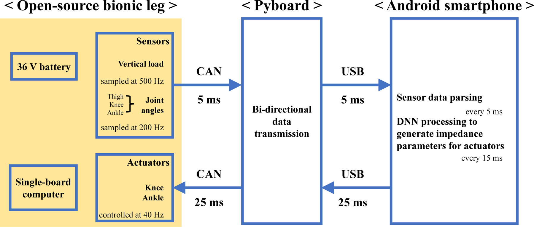
System configuration. Details of the OSL can be found in [18]. The Pyboard acted as a bidirectional translation module between the Android smartphone and OSL; it is connected to the OSL and the smartphone, respectively, by CAN and USB. The smartphone parses sensor data and generates impedance parameters every 5 ms and 15 ms, respectively. The generated impedance parameters are transmitted to the OSL and control the leg every 25 ms.

E. Experimental Protocol and Data Analysis

We quantified performance through an offline analysis of model fit and through real-time ambulation by non-amputees who walked with the OSL using a bypass adapter.

To quantify model fitting, the trained DNN models were applied to the benchmark dataset, and the Pearson correlation was calculated as follows:

$$\text{corr}\left(z_b,z_d\right)=\frac{1}{N-1}\sum _{i=1}^N\left(\frac{z_b^i-{\overline{z}}_d}{{\sigma }_{z_b}}\right)\left(\frac{z_d^i-{\overline{z}}_d}{{\sigma }_{z_d}}\right)$$ (7)

where z represents the synthetic impedance parameters (i.e., k, b, or θ^eq) obtained from ith benchmark data point $\left(z_b^i\right)$, and its estimated value $\left(z_d^i\right)$ using the DNNs. ${\overline{z}}_b$ and ${\overline{z}}_d$ denote the mean of z_b and z_d, respectively, and σ_z denotes the standard deviation of z.

For bypass testing, three individuals (AB1, AB2, and AB3) participated in a real-time ambulation experiment approved by the Northwestern University Institutional Review Board. The subjects performed level-ground walking with self-selected, long-, and short-step lengths with the parallel bars; 5 repetitions of each step length for each subject were performed. Next, we computed the root mean square difference (RMSD) between median joint trajectories (i.e., thigh, knee, and ankle) for the gait cycle: those from the benchmark dataset and those obtained from the bypass tests.

III. Results

A. Benchmark Data Fitting

Fig. 5 shows the trajectories of synthetic impedance parameters in the gait cycle from the benchmark dataset used for model training and their fitted data with the proposed model. The correlation for knee stiffness, ankle stiffness, knee damping coefficient, ankle damping coefficient, knee equilibrium angle, and ankle equilibrium angle was 0.89, 0.91, 0.78, 0.63, 0.98, and 0.89, respectively.

Fig. 5.

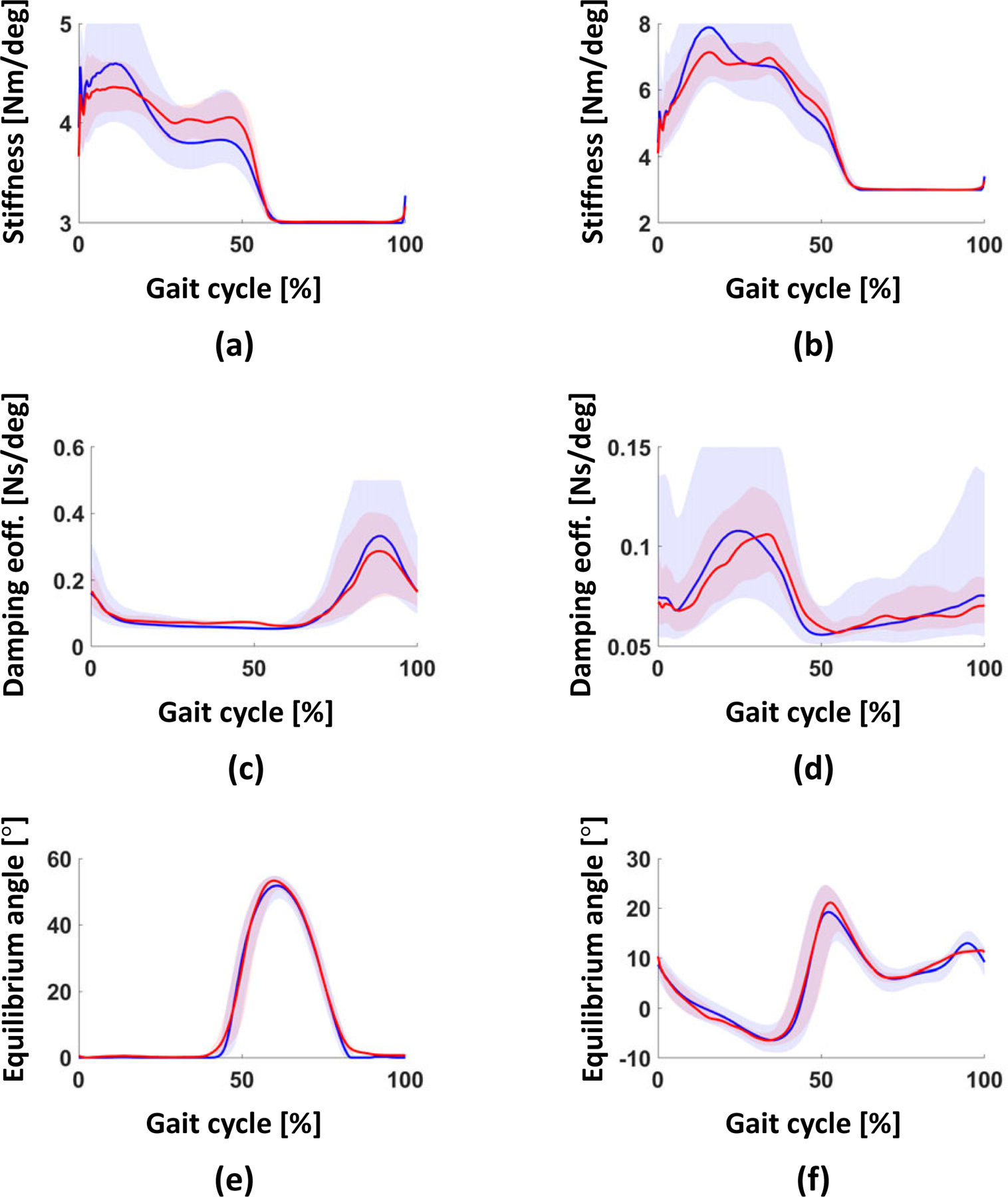
Comparison of synthetic impedance parameters from the benchmark data (blue lines) and their fitted data (red lines). The correlation was 0.89, 0.91, 0.78, 0.63, 0.98, and 0.89 for knee stiffness (a), ankle stiffness (b), knee damping coefficient (c), ankle damping coefficient (d), knee equilibrium angle (e), and ankle equilibrium angle (f), respectively. All plots show 75th and 25th percentiles in lighter bands.

B. Bypass Testing

Joint trajectories (i.e., thigh, knee, and ankle) from the benchmark dataset and bypass testing data in the gait cycle are shown in Fig. 6. All bypass testing subjects could ambulate within the level-ground walking mode with different step lengths; trajectories of the powered knee (Fig. 6(f)-(h)) and ankle (Fig. 6(j)-(l)) showed similar trajectories to those from the benchmark data (Fig. 6(e) and (i)). RMSDs between benchmark data and bypass testing data are shown in Table II.

Fig. 6.

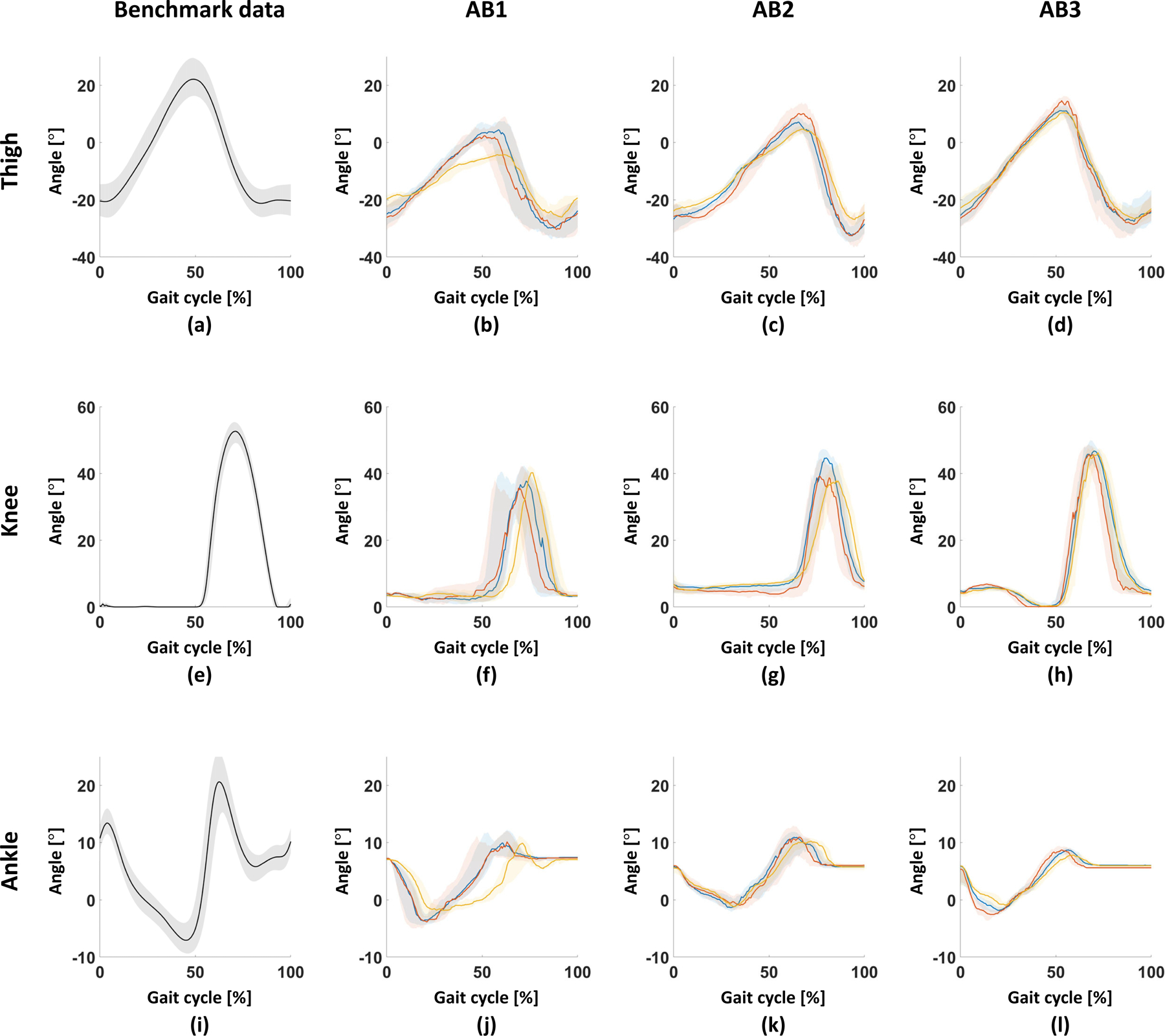
Joint trajectories in the gait cycle. From top to bottom, thigh, knee, ankle angles. From left to right, benchmark data, AB1, AB2, AB3. Knee and ankle angles of benchmark data ((e) and (i)) represent equilibrium angles. Blue, red, and yellow lines in bypass data (from the second column to the fourth column) represent trajectories at self-selected, long-, and short-steps, respectively. All plots show 75th and 25th percentiles in lighter bands.

TABLE II.

RMSD of joint angles with respect to the benchmark data.

RMSD [deg]		Subject
		AB1	AB2	AB3
Joint	Thigh	11.53	14.71	6.84
	Knee	9.59	15.33	6.44
	Ankle	5.79	5.41	7.17

There was a large difference in the range of thigh angle between benchmark data and bypass data, which might be induced by differences in sensor configuration, angular bias, or characteristics of subjects. In the case of the knee, RMSD increased as RMSD of thigh angle increased. On the other hand, in the case of the ankle, the differences were smaller than in the knee.

IV. Discussion

The proposed system learns a direct mapping from the sensor data on the prosthetic leg and modeled impedance parameters for the low-level controller to restore locomotion. Notably, the model was trained using gait trajectory from a benchmark dataset and did not use data from any of the subjects who ultimately ambulated with the OSL.

One of the challenges of this approach is converting the benchmark dataset to the domain expected by the OSL, which expects different sensor configurations (e.g., types of sensors, sensor coordinates, and data resolution). To compensate for the differences, we normalized the vertical load, removed the angle bias of the knee and ankle, and prevented knee flexion in the mid-stance by multiplying the knee angle by (1 − F_z)² before training. Although there was a large difference in thigh angle, we did not modify the thigh angle to minimize the modification in the input data for the DNN. These conversion parameters were heuristically chosen based on preliminary experiments. It is unclear to what extent these transformations would be necessary if a better domain adaptation strategy were used.

The ankle should provide powered push-off in the late stance phase of gait. In other words, the ankle should hit the ground at the end of the stance phase. However, the ankle usually tends to be dorsiflexed in the stance phase, so we commanded a sign-converted ankle angle $\left(\text{i}.\text{e}.,\hspace{0.17em}\hspace{0.17em}{\theta }_{ankle}^{eq}\hspace{0.17em}=\hspace{0.17em}-{\theta }_{ankle}^{pred}\right)$ to the leg as the equilibrium angle. Although this approach provided power to push-off, the resulting trajectory of the powered ankle was different from the actual human ankle trajectory (see Fig. 2 and Fig. 6). Therefore, a different mapping strategy could be considered to create more normal joint trajectories.

The stiffness and damping coefficients are important parameters to generate a reliable gait trajectory. We first attempted to simply impose constant stiffness and damping coefficients within the stance and swing phase of gait. However, subjects noted that ambulating with this style of control felt unrealistic and inconvenient; knee extension was too fast during the swing phase. One possible solution can be to impose constant parameters for each phase. However, we wanted to generate continuous impedance parameters by utilizing the benchmark dataset for more natural motion. Although several model-based methods have been proposed to predict joint stiffness [20], [21], we combined EMG data to generate synthetic stiffness and damping coefficients from benchmark data to simplify the relationship in accordance with the following criteria: stiffness should be proportional to user weight to support the leg in the stance phase; damping coefficient should be high when the joint is interacting with the ground (e.g., knee before and after the heel strike, or ankle before and after the midstance). Although EMG data can represent muscle stiffness, our synthetic parameters should not be considered ground truth and may differ from actual stiffness and damping coefficient. Ideally, the real impedance values for these joints (e.g., work of [22]) would be available for all joints and multiple activities. These may provide even better performances.

For the equilibrium angles, the ankle fitting performed more poorly than the knee. The ankle is relatively farther away from the thigh than the knee, and movement of the ankle might be highly related to not only thigh angle but also knee angle; these factors might have affected the performance. In the case of the stiffness and damping coefficient, the ankle damping coefficient showed poor-fitting performance because it has significant variation, as shown in Fig. 5(d). Nonetheless, the model achieved a good overall correlation with the median value.

Performance depends upon the DNN configuration. The Gaussian noise layer was critical in the proposed system. Without the Gaussian noise layer, oscillation increased in the swing phase of the OSL. Input signal (i.e., vertical load and thigh angle) corruption using the Gaussian noise layer may stabilize the leg by compensating for the difference in sensor configuration between the benchmark dataset and the OSL. The increase in the number of epochs seemingly increases stability, but we didn’t notice a significant difference. In this study, a 250 ms history of thigh angle and vertical load (i.e., the length of historical input data) was used to predict knee and ankle angles 100 ms in the future (i.e., the length of time in the future) as equilibrium angles. These parameters have a significant effect on performance. Regarding the length of historical input data, the longer the history used, the lower the sensitivity. For an even slightly longer history (i.e., 300 ms), difficulty in performing slow and short-step walking was encountered, although the LSTM layer was implemented in the networks. On the other hand, a short history, such as 50 ms, resulted in a jerky motion, especially in the swing phase. The length of time in the future determines the differences between current and equilibrium angles. If the differences are small (e.g., 50 ms in the future), the motor generates a small torque according to (1). Thus, the leg generates slower motion than the user intended; it may remain stiff in the worst case. On the other hand, a longer time length in the future results in faster leg motion due to the large torque generated. Meanwhile, stability is reduced. For example, in the transition from the stance phase to the swing phase, bypass subjects felt the leg moving too slowly for a prediction of 50 ms in the future; they felt that the knee was bent early in mid-stance for a prediction of 150 ms in the future.

Bypass testing results indicate that the proposed model successfully generated impedance parameters for gait in different step lengths. In addition, bypass subjects commonly noted that short-step walking performed very well. This is encouraged feedback because lower-limb amputation patients tend to walk with shorter step lengths than non-disabled individuals [23]. Future research will include testing with transfemoral amputation patients to demonstrate the proposed method. In addition, a more detailed analysis in terms of naturalness and symmetricity between sound and prosthetic sides will be performed.

Although the benchmark dataset we used contains various ambulation modes, including stair ascent/descent and ramp ascent/descent, we used only treadmill data and demonstrated level-ground walking since data, not from the treadmill, provides only partial vertical load during gait. We believe that the proposed model can cover the various ambulation modes with an additional dataset, and it will be performed as future work.

Our study had several limitations in terms of quantitative analysis. First, although all bypass subjects who participated in this study could walk at different speeds and different step lengths, the results were not quantitated. Additional tests, such as walking on the treadmill at different speeds consistent with the benchmark data, should be needed for the generalizability of the proposed method. To guarantee the safety and reliability of the proposed system, we performed a T-handle test prior to the bypass test (see supplementary video); the T-handle test refers to a test in which a T-shaped handle is attached to the OSL, and locomotion is mimicked by hand. We investigated whether the system could provide sufficient support during a stance, as well as avoid unstable leg oscillation and any jerky motion (e.g., sudden knee drop in the stance phase). No such problems were observed. However, this qualitative evaluation may not be sufficient because safety remains a primary concern. Future research will include a quantitative evaluation of safety under well-organized conditions.

V. Conclusion

In this study, we proposed the benchmark data-derived DNN model to control prosthetic legs. The proposed DNN successfully generated impedance parameters for level-ground walking trained using synthetic impedance parameters from non-disabled limb trajectories.

The high correlation between synthetic impedance parameters and their fitted parameters with benchmark data confirmed hypothesis (i). The proposed DNN accomplished comfortable and reliable locomotion without post-tuning the system for three bypass subjects, confirming the hypothesis (ii).

References

- [1].Moxey P, Gogalniceanu P, Hinchliffe R, Loftus I, Jones K, Thompson M, and Holt P, “Lower extremity amputations—a review of global variability in incidence,” Diabetic Medicine, vol. 28, no. 10, pp. 1144–1153, 2011. [DOI] [PubMed] [Google Scholar]
- [2].McDonald CL, Westcott-McCoy S, Weaver MR, Haagsma J, and Kartin D, “Global prevalence of traumatic non-fatal limb amputation,” Prosthetics and orthotics international, p. 0309364620972258, 2021. [DOI] [PubMed] [Google Scholar]
- [3].Goldfarb M, Lawson BE, and Shultz AH, “Realizing the promise of robotic leg prostheses,” Science translational medicine, vol. 5, no. 210, pp. 210ps15–210ps15, 2013. [DOI] [PubMed] [Google Scholar]
- [4].Thatte N and Geyer H, “Toward balance recovery with leg prostheses using neuromuscular model control,” IEEE Transactions on Biomedical Engineering, vol. 63, no. 5, pp. 904–913, 2015. [DOI] [PMC free article] [PubMed] [Google Scholar]
- [5].Villarreal DJ, Poonawala HA, and Gregg RD, “A robust parameterization of human gait patterns across phase-shifting perturbations,” IEEE Transactions on Neural Systems and Rehabilitation Engineering, vol. 25, no. 3, pp. 265–278, 2016. [DOI] [PMC free article] [PubMed] [Google Scholar]
- [6].Simon AM, Ingraham KA, Fey NP, Finucane SB, Lipschutz RD, Young AJ, and Hargrove LJ, “Configuring a powered knee and ankle prosthesis for transfemoral amputees within five specific ambulation modes,” PloS one, vol. 9, no. 6, p. e99387, 2014. [DOI] [PMC free article] [PubMed] [Google Scholar]
- [7].Huang H, Crouch DL, Liu M, Sawicki GS, and Wang D, “A cyber expert system for auto-tuning powered prosthesis impedance control parameters,” Annals of biomedical engineering, vol. 44, no. 5, pp. 1613–1624, 2016. [DOI] [PubMed] [Google Scholar]
- [8].Wen Y, Si J, Brandt A, Gao X, and Huang HH, “Online reinforcement learning control for the personalization of a robotic knee prosthesis,” IEEE transactions on cybernetics, vol. 50, no. 6, pp. 2346–2356, 2019. [DOI] [PubMed] [Google Scholar]
- [9].Kang I, Molinaro DD, Duggal S, Chen Y, Kunapuli P, and Young AJ, “Real-time gait phase estimation for robotic hip exoskeleton control during multimodal locomotion,” IEEE Robotics and Automation Letters, vol. 6, no. 2, pp. 3491–3497, 2021. [DOI] [PMC free article] [PubMed] [Google Scholar]
- [10].Ren J-L, Chien Y-H, Chia E-Y, Fu L-C, and Lai J-S, “Deep learning based motion prediction for exoskeleton robot control in upper limb rehabilitation,” in 2019 International Conference on Robotics and Automation (ICRA). IEEE, 2019, pp. 5076–5082. [Google Scholar]
- [11].Hu B, Simon AM, and Hargrove L, “Deep generative models with data augmentation to learn robust representations of movement intention for powered leg prostheses,” IEEE Transactions on Medical Robotics and Bionics, vol. 1, no. 4, pp. 267–278, 2019. [DOI] [PMC free article] [PubMed] [Google Scholar]
- [12].Teh Y and Hargrove LJ, “Using latent representations of muscle activation patterns to mitigate myoelectric interface noise,” in 2021 10th International IEEE/EMBS Conference on Neural Engineering (NER). IEEE, 2021, pp. 1148–1151. [Google Scholar]
- [13].Eslamy M, Oswald F, and Schilling AF, “Estimation of knee angles based on thigh motion: A functional approach and implications for high-level controlling of active prosthetic knees,” IEEE Control Systems Magazine, vol. 40, no. 3, pp. 49–61, 2020. [Google Scholar]
- [14].Liang J, Shi Z, Zhu F, Chen W, Chen X, and Li Y, “Gaussian process autoregression for joint angle prediction based on semg signals,” Frontiers in Public Health, vol. 9, p. 567,2021. [DOI] [PMC free article] [PubMed] [Google Scholar]
- [15].Jahanandish MH, Fey NP, and Hoyt K, “Lower limb motion estimation using ultrasound imaging: A framework for assistive device control,” IEEE journal of biomedical and health informatics, vol. 23, no. 6, pp. 2505–2514, 2019. [DOI] [PMC free article] [PubMed] [Google Scholar]
- [16].Rabe KG and Fey NP, “Evaluating electromyography and sonomyography sensor fusion to estimate lower-limb kinematics using gaussian process regression,” Frontiers in Robotics and AI, vol. 9, 2022. [DOI] [PMC free article] [PubMed] [Google Scholar]
- [17].Camargo J, Ramanathan A, Flanagan W, and Young A, “A comprehensive, open-source dataset of lower limb biomechanics in multiple conditions of stairs, ramps, and level-ground ambulation and transitions,” Journal of Biomechanics, vol. 119, p. 110320, 2021. [DOI] [PubMed] [Google Scholar]
- [18].Azocar AF, Mooney LM, Duval J-F, Simon AM, Hargrove LJ, and Rouse EJ, “Design and clinical implementation of an open-source bionic leg,” Nature biomedical engineering, vol. 4, no. 10, pp. 941–953, 2020. [DOI] [PMC free article] [PubMed] [Google Scholar]
- [19].Marieb E, Brady P, Wilhelm P, and Mallatt J, Human Anatomy, Global Edition, 9th ed. London, England: Pearson Education, aug 2019. [Google Scholar]
- [20].Sartori M, Maculan M, Pizzolato C, Reggiani M, and Farina D, “Modeling and simulating the neuromuscular mechanisms regulating ankle and knee joint stiffness during human locomotion,” Journal of neurophysiology, vol. 114, no. 4, pp. 2509–2527, 2015. [DOI] [PMC free article] [PubMed] [Google Scholar]
- [21].Misgeld BJ, Zhang T, Luken MJ, and Leonhardt S, “Model-based estimation of ankle joint stiffness,” Sensors, vol. 17, no. 4, p. 713, 2017. [DOI] [PMC free article] [PubMed] [Google Scholar]
- [22].Lee H, Rouse EJ, and Krebs HI, “Summary of human ankle mechanical impedance during walking,” IEEE journal of translational engineering in health and medicine, vol. 4, pp. 1–7, 2016. [DOI] [PMC free article] [PubMed] [Google Scholar]
- [23].Su P, Gard SA, Lipschutz RD, and Kuiken TA, “Gait characteristics of persons with bilateral transtibial amputations,” Journal of rehabilitation research and development, vol. 44, no. 4, p. 491, 2007. [DOI] [PubMed] [Google Scholar]
Associated Data
This section collects any data citations, data availability statements, or supplementary materials included in this article.