BALSA: Bayesian algorithm for local sequence alignment

Abstract

The Smith–Waterman algorithm yields a single alignment, which, albeit optimal, can be strongly affected by the choice of the scoring matrix and the gap penalties. Additionally, the scores obtained are dependent upon the lengths of the aligned sequences, requiring a post-analysis conversion. To overcome some of these shortcomings, we developed a Bayesian algorithm for local sequence alignment (BALSA), that takes into account the uncertainty associated with all unknown variables by incorporating in its forward sums a series of scoring matrices, gap parameters and all possible alignments. The algorithm can return both the joint and the marginal optimal alignments, samples of alignments drawn from the posterior distribution and the posterior probabilities of gap penalties and scoring matrices. Furthermore, it automatically adjusts for variations in sequence lengths. BALSA was compared with SSEARCH, to date the best performing dynamic programming algorithm in the detection of structural neighbors. Using the SCOP databases PDB40D-B and PDB90D-B, BALSA detected 19.8 and 41.3% of remote homologs whereas SSEARCH detected 18.4 and 38% at an error rate of 1% errors per query over the databases, respectively.

INTRODUCTION

Biopolymer sequence comparison methods are the most commonly used tools in bioinformatics. Popular sequence alignment algorithms include SSEARCH, an optimal dynamic programming algorithm, and FASTA and BLAST, two fast heuristic algorithms. Among the three, SSEARCH has been demonstrated on several occasions to find the most homologs in a protein database search (1,2). Local dynamic programming and heuristic methods were significant advances in biological sequence analyses. However, these algorithms require the specification of a scoring matrix and a set of gap penalties, and return only a single alignment and an associated score that must be adjusted for the lengths of the sequences. Bayesian statistics provides a means to relax these requirements and to achieve an automatic length adjustment. Furthermore, since all required sums can be completed using a modified dynamic programming method, exact inferences on all variables are available.

Optimization algorithms

Local alignment is typically the method of choice for aligning a pair of biopolymers; obtaining the best common subsequence is usually more advantageous to detect distantly related proteins than an alignment end to end, globally (3–5). In an effort to overcome the issue of specifying gap penalties, Sankoff (6) developed a constrained optimization algorithm that produces the optimal alignment subject to the constraint that there are no more than k aligned blocks, extending the concept of local alignment; the portions of the sequences that are not included in the aligned blocks are completely ignored. However, the specification of the number of aligned blocks, or equivalently the number of gaps, brings up a similar issue as with traditional alignment algorithms.

Bayesian algorithms

There is one case in which Bayesian inference methods have been used to develop a sequence alignment algorithm, the ‘Bayes Block Aligner’. The ‘Bayes Block Aligner’ is a local alignment algorithm based on Sankoff’s method, which returns the posterior distribution of all alignments considering all the selected gapping and scoring matrices, weighing each in proportion to its posterior probability based on the data. The ‘Bayes Block Aligner’ outperformed the optimized SSEARCH on VAST pdb25, pdb35 and pdb45 alignments (7). Subsequently, Liu and Lawrence (8) described a Bayesian approach for global sequence alignment. In this work, we show how to formulate a Bayesian local sequence alignment algorithm (BALSA).

Bayesian inference

A more complete overview of Bayesian statistics in respect to bioinformatics was given by Liu and Lawrence (8); below is a brief summary. Let θ denote the set of unknown parameters, such as the gap penalties, and let y_obs denote the observed data, such as the sequence data. The likelihood function is defined as the probability of the observed data given the unknown parameters: L(θ; y_obs) = P(y_obs │ θ). Thus, the joint probability distribution of θ and y_obs is defined as:

Joint = likelihood*prior

P(y_obs, θ) = L(θ; y_obs)P(θ) = P(y_obs │ θ)P(θ)

The Bayesian inference is made by obtaining and inspecting the posterior distributions of the unknown quantities of interest, where the posterior distributions are obtained from Bayes theorem, i.e. P(θ │ y_obs) = P(y_obs, θ) / P(y_obs), where P(y_obs) is computed by integrating over θ in the joint distribution (9). Suppose the unknown parameter is of n dimensions, i.e. θ = (θ₁, ..., θ_n). Those parameter components that are not of immediate interest but necessary to the model need to be integrated out from the joint distribution so as to provide a proper inference on the unknown variable of interest, for example θ₁:

P(θ₁ │ y_obs) = [∫···∫ P(y_obs │ θ₁, ..., θ_n) P(θ₁, ..., θ_n)dθ₂···dθ_n] /

[∫···∫ P(y_obs │ θ₁, ..., θ_n) P(θ₁, ..., θ_n) dθ₁···dθ_n]

Lastly, the appropriateness of the model must be evaluated. From this step, improvements in the model may be suggested and the process repeated.

MATERIALS AND METHODS

The premise behind our Bayesian analysis is that all quantities related to the alignment task are treated as random variables, observed data, missing data and unknown parameters alike. For a pair of sequences, the observed data are R⁽¹⁾ = {R₁⁽¹⁾ ...R_I⁽¹⁾} and R⁽²⁾ = {R₁⁽²⁾ ...R_J⁽²⁾}. Let A be a matrix that characterizes an alignment whose (i, j)-entry is defined as:

Thus, two natural constraints have to be satisfied: A_ij ≤ 1 and A_ij ≤ 1. We use Θ to denote a set of matrices analogous to scoring matrices such as BLOSUM (10) or PAM (11), where Θ(r¹, r²) is defined as the joint distribution of a pair of aligned residues, Θ(r¹, H) and Θ(H, r²), the marginal distributions. Typical scoring matrices correspond to the logarithm of residue interactions:

log= log Θ(r_i¹, ) – log Θ(r_i¹, H) – log Θ(H, )

Lastly, Λ = (λ_o, λ_e) is a set of predefined gap odds ratios comparable with traditional gap penalties where the penalty for opening and extending a gap is log(λ_o) and log(λ_e), respectively (7,8,12). Although the scoring matrices and gap penalties utilized in the algorithm are odds ratios, as BALSA will calculate the sums of probability ratios, they will be given throughout the paper in the traditional manner; scoring matrices expressed as BLOSUMs and gap penalties in halfbits in order to keep consistency with the earlier evaluation on SSEARCH.

Joint, likelihood and priors

Most sequence alignment methods can be viewed as optimizing an objective function, some of which can be viewed as a log-likelihood (2,8). This requires the user to set specific parameter values, Θ^ο and Λ^ο, in order to find the optimal alignment, A*, over all possible alignments. Mathematically this is equivalent to computing:

{log P(P(R⁽¹⁾, R⁽²⁾ │ A, Θ^ο) + log P(A │ Λ)^ο}

The Bayesian procedure avoids prefixed Θ and Λ by allowing for an integration over a range of possible gap penalty values and scoring matrices. More precisely, the full joint distribution, Joint = likelihood*priors, can be defined as:

P(R⁽¹⁾, R⁽²⁾, A, Θ, Λ) = P(R⁽¹⁾, R⁽²⁾ │ A, Θ)P(A │ Λ)P(Θ, Λ)

where we can write

log P(R⁽¹⁾, R⁽²⁾ │ A, Θ) =log Θ(r_i¹, H) +log Θ(H, )

+a_ij log

Prior probability distributions can be used to incorporate previous knowledge about the parameters. Since we lack quantifiable information in this case, uniform priors are employed. That is, all scoring matrix and gap penalty pairs, (Θ, Λ), are equally likely a priori, i.e. P(Θ, Λ) = 1 / N_{Θ, Λ}, where N_{Θ, Λ} is the number of scoring matrix gap penalty pairs in the chosen series. Let P(A │ Λ) be the probability of any allowable path A prior to seeing the sequence data. Then, we have:

P(A │ λ_o, λ_e) =

where k_g(A) is the total number and l_g(A) is the length of the gaps in A (8). The summation in the denominator is over all possible alignments A′ in the two sequences beginning at any point and ending at any point under the constraint that the alignment must start before it ends.

Posteriors

The unknown variable A can be removed from the joint distribution by summing over all alignments as follows:

P(R⁽¹⁾, R⁽²⁾ │ Θ, Λ) =(R⁽¹⁾, R⁽²⁾ │ A, Θ)P(A │ λ_o, λ_e)

= 1

Then by the Bayes rule, the desired posterior distribution of the gap parameters and the scoring matrix can be obtained:

P(Θ, Λ │ R⁽¹⁾, R⁽²⁾) = 2

Similarly, the posterior distribution for an alignment A* can be expressed mathematically as:

P(A* │ R⁽¹⁾, R⁽²⁾) = 3

Given that the number of possible alignments for even small biopolymer sequences is immense, it is not feasible to calculate this distribution in a brute force manner, but equation 3 can be calculated for any given path and a representative sample of alignments can be drawn using a sampling backtrace algorithm. Furthermore, the denominator of equation 2 gives the marginal probability of the data, the so-called Bayes factor (9), which can be used to judge whether the two sequences should be aligned or treated independently.

Algorithm

The Bayesian model must capture the idea of local alignment, i.e. aligning the related subsequences and ignoring the unrelated sections of the sequence on the ends. The summation over all alignments needs to take into account all alignments that begin at any point and end at any point in the two sequences while adhering to the constraint that an alignment may not end before it has begun. In this section we describe how this summation over all alignments can be achieved via a recursive algorithm.

Recursive algorithm

Completing the sums in the numerator of equation 1. At each step of the algorithm, the partial sum up to residues i and j in sequences 1 and 2, respectively, contains five components: match residues r_i⁽¹⁾ and r_j⁽²⁾, insertion in sequence 1, deletion in sequence 1, start alignment at r_i⁽¹⁾ and r_j⁽²⁾, and end alignment at r_i⁽¹⁾ and r_j⁽²⁾. In addition, the assumption that a deletion may not be followed by an insertion and vice versa is made in order to only take into account distinct alignments. Typically in sequence alignment models the interaction term is used instead of the joint probability term, Θ(r_i⁽¹⁾, r_j⁽²⁾). Thus, Θ(r_i⁽¹⁾, r_j⁽²⁾) can be replaced by Ψ(r_i⁽¹⁾, r_j⁽²⁾) and Θ(r_i⁽¹⁾, H) and Θ(H, r_j⁽²⁾) replaced by 1. The algorithm can be written as follows:

(i) A match at r_i⁽¹⁾ and r_j⁽²⁾ can follow a match, insertion, deletion or new alignment from partial sums with indices (i – 1, j – 1):

Pm(i, j) = {Pm(i – 1, j – 1) + Pi(i – 1, j – 1) + Pd(i – 1, j – 1)

+ Pn(i – 1, j – 1)}Ψ (r_i⁽¹⁾, r_j⁽²⁾)

(ii) An insertion in sequence 1 can only follow partial sums with indices (i – 1, j). In addition, an insertion may not follow a deletion. If the last move was an insertion, then a gap is being extended, λ_e. On the other hand, if the last move was a match, either continued or the beginning of a new alignment, a new gap is being introduced, λ_o:

Pi(i, j) = λ_ePi(i – 1, j) + λ_o{Pm(i – 1, j) + Pn (i – 1, j)}

(iii) Accordingly, the same follows for a deletion:

Pd(i, j) = λ_ePd(i, j – 1) + λ_o{Pm(i, j – 1) + Pn(i, j – 1)}

(iv) Starting an alignment at r_i⁽¹⁾ and r_j⁽²⁾ is matching those two residues as if they are the first two residues in the sequences:

Pn(i, j) = Ψ(r_i⁽¹⁾, r_j⁽²⁾)

(v) The partial sum of ending at r_i⁽¹⁾ and r_j⁽²⁾ is the sum of all possible paths beginning anywhere prior to r_i⁽¹⁾ and r_j⁽²⁾ and ending at r_i⁽¹⁾ and r_j⁽²⁾:

Pe(i, j) = Pm(i, j) + Pi(i, j) + Pd(i, j) + Pn(i, j)

(vi) Finally, the partial sum of all alignments beginning at any point prior to r_i⁽¹⁾ and r_j⁽²⁾ is the sum of all possible paths ending at any point prior to and including r_i⁽¹⁾ and r_j⁽²⁾:

P(i, j) =Pe(k, l)

Thus, at the end of the recursion, we have:

P(R⁽¹⁾, R⁽²⁾, │ A, Θ)λ_o^kg(A)λ_e^{lg(A) – kg(A)}

= P(I, J)Θ(R⁽¹⁾, H)Θ(H, R⁽²⁾)

The initial conditions are: Pm(i, 0), Pi(i, 0), Pd(i, 0), Pn(i, 0) and Pe(i, 0) = 0 ∀i and Pm(0, j), Pi(0, j), Pd(0, j), Pn(0, j) and Pe(0, j) = 0 ∀j.

Completing the sums in the denominator of equation 1. This can be computed in a similar manner as the recursive algorithm above:

Nm(i, j) =  Nm(i – 1, j – 1) + Ni(i – 1, j – 1) + Nd(i – 1, j – 1) +

Nn(i – 1, j – 1)

Ni(i, j) = λ_eNi(i – 1, j) + λ_o{Nm(i – 1, j) + Nn(i – 1, j)}

Nd(i, j) = λ_e Nd(i, j – 1) + λ_o{Nm(i, j – 1) + Nn(i, j – 1)}

Nn(i, j) = 1

Ne(i, j) = Nm(i, j) + Ni(i, j) + Nd(i, j) + Nn(i, j)

N(i, j) =Ne(k, l)

The initial conditions are the same as for the recursive algorithm for the numerator. From the above summations, the exact posterior distribution for Θ and Λ can be calculated according to equation 2.

Backward recursive sampling algorithm

The backward recursive algorithm for sampling alignments from their exact posterior distribution is comparable with the algorithm used by the ‘Bayes Aligner’ to obtain the posterior alignment distribution (7). Sampling an alignment can be broken down into three steps:

(i) The parameters Θ and Λ are sampled from their exact posterior distribution, P(Θ, Λ │ R⁽¹⁾, R⁽²⁾), obtained from the forward algorithm.

(ii) Conditioning on Θ and Λ, an endpoint from which to start the backtrace is sampled. In local dynamic programming algorithms, this is simply the maximum of the matrix obtained from the forward sum, but in Bayesian methods, this is a sample from all the possible end points. Thus, the end point (k, l) from which to begin the backward recursion is chosen from all Pe(i, j): i = 1, ..., I; j = 2, ..., J. From the sampled endpoint (k, l) the next move is sampled from four choices, matching, inserting, deleting or beginning the alignment at (k, l), according to the probabilities, Pm(k, l) / Pe(k, l), Pi(k, l) / Pe(k, l), Pd(k, l) / Pe(k, l) and Pn(k, l) / Pe(k, l), respectively.

(iii) Afterwards, each choice now depends on the previous one:

(a) If the last choice was a match, Pm(k, l), r_k⁽¹⁾ and r_l⁽²⁾ are matched and (k, l) becomes (k – 1, l– 1). One proceeds by taking one of the four choices, match, insert, delete or begin alignment, according to the probabilities, Pm(k, l) / Pe(k, l), Pi(k, l) / Pe(k, l), Pd(k, l) / Pe(k, l) and Pn(k, l) / Pe(k, l), respectively.

(b) If the last choice was an insert, a gap is inserted into sequence 1 and (k, l) becomes (k – 1, l). An insert may be preceded by three of the four choices, match, insert or begin alignment. The next choice is sampled from the probabilities, Pm(k, l) / [Pm(k, l) + Pi(k, l) + Pn(k, l)], Pi(k, l) / [Pm(k, l) + Pi(k, l) + Pn(k, l)] and Pd(k, l) / [Pm(k, l) + Pi(k, l) + Pn(k, l)].

(c) Similarly, if the last choice was a delete, (k, l) becomes (k, l – 1). The next choice is sampled from the probabilities, Pm(k, l) / [Pm(k, l) + Pd(k, l) + Pn(k, l)], Pd(k, l) / [Pm(k, l) + Pd(k, l) + Pn(k, l)] and Pn(k, l) / [Pm(k, l) + Pd(k, l) + Pn(k, l)].

(d) If the last choice was to begin a new alignment, r_k⁽¹⁾ and r_l⁽²⁾ are matched. Since this is the beginning of the alignment, similar to that 0 being the best choice in a local dynamic programming backward algorithm, all upstream residues are ignored and the sample is completed.

Availability

The software for BALSA is available at http://www.wadsworth.org/resnres/bioinfo/

RESULTS

The performance of sequence alignment algorithms has been evaluated and compared on several occasions. The two most extensive comparisons were by Pearson and Lipman (13) and Brenner et al. (1). Brenner et al. used SCOP, a database of proteins of known structure and function, to compare FASTA (13), BLAST (14) and SSEARCH. They found SSEARCH with optimally chosen gap penalties and E()-values to outperform the others, correctly identifying the most remote homologs in the database. Pearson and Lipman’s comparison was similar, but based on superfamilies in the Protein Information Resource. Again SSEARCH was found to outperform the other procedures.

In order to keep consistency with earlier evaluations, the same databases used by Brenner et al. (1), PDB40D-B and PDB90D-B, were employed in the evaluation of our alignment procedure, BALSA. PDB40D-B and PDB90D-B include only domains <40 and <90% identical to any of the others and contain 1323 and 2079 domains, respectively. In an all-versus-all comparison there are 1 749 006 ordered pairs of which ∼9044 (0.5%) are structurally related for PDB40D-B. PDB90D-B consists of 4 320 162 ordered pairs of which 53 988 (∼1.2%) are distantly related (1). The analysis of our algorithm is broken down into two parts, evaluation and performance. First, we will address the dynamic programming issues including the setting of parameters and length adjustments of optimal scores. Subsequently, its ability to detect remote protein homologs is compared with SSEARCH with E()-values. The selection of scoring matrices and gap penalties to be utilized by BALSA was determined by taking the set of 10 combinations of scoring matrices and gap penalties previously identified by Brenner to find the most structural homologs on the SCOP database (15). The examination of all 10 of these showed little improvement in coverage by the addition of matrices beyond the following four; BLOSUM matrix/gap opening penalty/gap extension penalty: 45/–12/–1, 50/–12/–2, 62/–10/–1 and 62/–12/–1. The set that was found to perform best on SSEARCH was BLOSUM 45/–12/–1. Brenner et al. used it in a previous comparison of SSEARCH to FASTA and BLAST on PDB40D-B and PDB90D-B (1).

Addressing dynamic programming issues

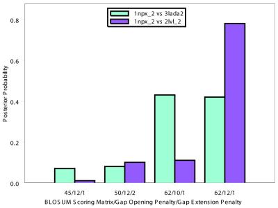
Preselection of scoring matrices and gap parameters. In the majority of cases we found that the posterior distribution over the BLOSUM series of scoring matrices was close to uniform. However, in 21.4% of cases, the probability for one or several of these gap/matrix combinations deviated from the uniform, >2-fold, in at least one set. For example, as Figure 1 demonstrates, very different posterior distributions were obtained for the protein 1npx_2, NADH peroxidase, with two of its homologs, 3lada2 and 1lvl_2, both dihydrolipoamide dehydrogenases. The large posterior probabilities for 1npx_2 versus 3lada2 for the second and third scoring-gap pairs demonstrate that these score-gap pairs yield much larger scores from the algorithm, likewise for 1npx_2 versus 2lvl_2 given the fourth scoring-gap pair. Furthermore, if only the third set of matrix/gap pairs are used, 1npx_2 versus 2lvl_2 does not obtain a score large enough to be detected as a homologous pair but 1npx_2 versus 3lada2 does at a 1% errors per query (EPQ). The first and second matrix/gap pairs do not detect either homologous pair and the fourth detects both. Effects of such variations on detection of homologs are given in the Evaluation method section below.

Figure 1.

BALSA allows multiple matrices and gap parameters to be input, returning the posterior distribution over all selected parameters, P(Θ, Λ │ R⁽¹⁾, R⁽²⁾). Four matrix gap parameter pairs, BLOSUM matrix/λ_o/λ_e, were chosen based on their performance on sample data: (i) 45/–12/–1, (ii) 50/–12/–2, (iii) 62/–10/–1 and (iv) 62/–12/–1. This histogram of the exact posterior distribution probabilities demonstrates that the selection of scoring matrix and gap parameters is highly dependent upon the given sequences.

Length dependence. A major development in optimal local sequence alignment was the development of probabilistic scoring schemes to take into account the dependence of score on the lengths of the two sequences. This usually involves fitting a curve to the distribution of the scores of the true negatives in a database versus the log product of the sequence lengths. This allows the significance of a given alignment to be expressed in terms of a P-value or E()-value (2,16–19). For example, SSEARCH raw scores obtained 10.5% coverage at a 1% EPQ whereas SSEARCH with E()-values yielded 18.4% at the same cut-off. BALSA includes terms that adjust for variations in sequence length. Specifically, the denominator of the likelihood function

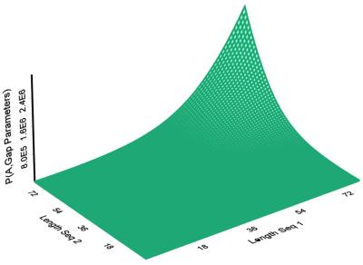
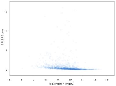
is only dependent upon the lengths of the two sequences, not the amino acid sequences. As seen in Figure 2, the sum over all alignments grows larger as the lengths of the two sequences increase. Figure 3 indicates that there is little dependence of the score on sequence length. To examine this adjustment more quantitatively, a least-squares line was fit to BALSA score as a function of the lengths of the sequences. The analysis was performed on the Score versus the two independent variables, Length1 and Length2, and likewise the Score versus log(Length1*Length2). The analysis returned correlation coefficients of 0.008699 and 0.01431, respectively.

Figure 2.

The denominator of the likelihood,

, does not depend on amino acid sequences of the proteins. The plot of the denominator versus a pair of sequences increases as their lengths increase, inherently correcting for sequence length with the algorithm.

Figure 3.

The plot of the score from BALSA versus log(Length1*Length2) returns a correlation coefficient of 0.01431 from the least-squares analysis. This demonstrates that there is little dependence of score on the lengths of sequences 1 and 2, respectively.

Comparison with SSEARCH

Evaluation method. An all-versus-all comparison of the database was conducted using BALSA, the results were sorted in descending order, and a cut-off was drawn at which the number of related sequences above the threshold was acceptable with a given error rate (number of false positives). The various thresholds and related errors were evaluated by utilizing coverage versus error plots as in Brenner et al. (1). The coverage corresponds to the fraction of homologs detected at a specified error rate (EPQ), which is the number of non-homologs above the cut-off divided by the total number of query sequences.

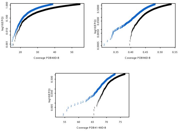
BALSA versus SSEARCH. In previous studies SSEARCH with E()-values detected 18.4 and 38% of homologous pairs at a 1% EPQ on PDB40D-B and PDB90D-B with parameters found to be optimal, BLOSUM 45 and gap penalties –12 and –1 (1,15). BALSA, with the set of four matrix/gap penalty pairs previously defined, obtained 19.8 and 41.3% of all relationships at the same error rate for the two respective databases. In evaluating the non-overlapping sequences between the two databases (sequences with between 41 and 90% sequence identity) an even larger increase in detecting homologous pairs was noted; 60% for SSEARCH to 67.2% for BALSA at a 1% EPQ. In fact, as seen in Figure 4, BALSA outperformed SSEARCH at all EPQ levels for all three databases. In evaluating the individual contribution of each of the matrix/gap penalty pairs, we found that most of the gain was from one pair. The coverage was increased by 0.3% from one to four matrices and 0.03% from two to four matrices for the PDB40D-B databases, less for PDB41-90D-B and PDB90D-B. The optimal single set of parameters used by SSEARCH are BLOSUM 45/–12/–1 and they produce coverages of 18.4, 38 and 60% at a 1% EPQ for PDB40D-B, PDB90D-B and PDB41-90D-B, respectively. The application of the same parameters to BALSA resulted in an increase to 19.2, 41.5 and 67.0% at the same error rate on the three databases. The single set parameters that found the highest coverage for BALSA are BLOSUM 62/–12/–1, finding 19.5, 41.2 and 67% at a 1% EPQ for the respective databases.

Figure 4.

Coverage versus EPQ plots of BALSA with the four given matrix gap parameter pairs and SSEARCH with optimal gap parameters and E()-values. BALSA obtained a larger coverage, detection of more homologous pairs, than SSEARCH at all EPQ levels for PDB40D-B, PDB90D-B and PDB41-90D-B.

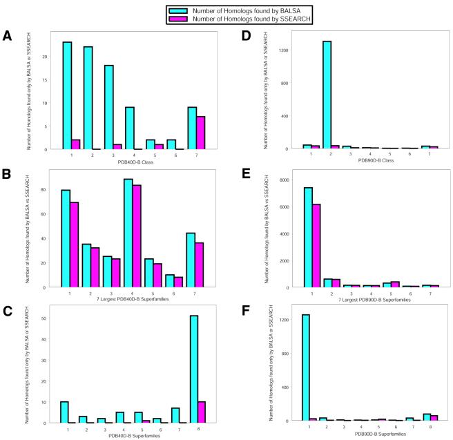
The SCOP database is broken down into classes, folds, superfamilies, families and domains. PDB40D-B and PDB90D-B consist of seven classes, 346 folds and 474 superfamilies. The number of proteins per class ranges substantially from 27 to 318 proteins, as does the number of structural homologs per class, 49–1797, for PDB40D-B. There are 33–620 proteins and between 89 and 19 529 homologs per class for PDB90D-B. To address potential biases that could arise from these substantial differences, we examined the number of structural neighbors found by each algorithm for each of the seven classes and the seven largest superfamilies, the level at which homology is defined, using the standard scoring scheme, BALSA 45/–12/–1. To examine the differences of behavior by class we examined the structural neighbors returned by one algorithm but not the other. BALSA finds 74 more structural neighbors than SSEARCH. Of the total number of homologs returned by each algorithm, 85 are unique to BALSA and 11 are unique to SSEARCH. As shown in Figure 5A, BALSA gains are in all classes with its smallest proportionate gain in class 7. We also examined the number of hits at the superfamily level. We found that 45.2% of the homologs for PDB40D-B fell into the seven superfamilies that have the largest numbers of homologs. Both algorithms found proportionately fewer structural neighbors than expected (35.5% for BALSA and 34.5% for SSEARCH) in these seven superfamilies. The specific number of the structural homologs found by each algorithm in these largest seven superfamilies are shown in Figure 5B. BALSA again finds more homologs than SSEARCH in all seven superfamilies. A comparison of structural neighbors unique to each algorithm was completed but is sparse. Only 34 of the 85 homologous pairs found by BALSA and one of the 11 homologous pairs unique to SSERACH fall into one of these seven largest superfamilies. As shown in Figure 5C, BALSA finds more homologs in each superfamily, with its advantage reasonably distributed over the seven largest superfamilies. As seen in the eighth category, the remaining superfamilies, the majority of the gain observed by BALSA is not in the largest seven superfamilies. In addition, the overall proportion of homologs identified uniquely by BALSA within the seven largest superfamilies (40%) is somewhat lower than the proportion in PDB40D-B (45.2%). The removal of the seven largest superfamilies from the analysis resulted in an increase in coverage for both algorithms, 18.4–25.1% for SSEARCH and 19.2–27.0% for BALSA, raising the improvement of BALSA over SSEARCH from 0.8 to 1.9%. An equivalent analysis was completed for PDB90D-B: the comparison of the number of homologs found by each algorithm for each class and the largest seven superfamilies. For proteins detected by only one of the algorithms, BALSA finds 1312 more structural neighbors than SSEARCH. There are 1412 structural neighbors identified only by BALSA and 100 detected only by SSEARCH, and most of BALSAs gain is concentrated in class two, Figure 5D. As before, we restrict the view to the seven superfamilies that contain the most homologous pairs. 78.7% of the total homologs found by BALSA fall into one of the seven largest superfamilies, 76.9% for SSEARCH, in comparison with 76.1% for PDB90D-B. The specific number of homologs that fall into each of these superfamilies is shown in Figure 5E. In this case, unlike our results for PDB40D-B, the vast majority of the homologous pairs identified by BALSA, and to a somewhat lesser extent by SSEARCH, is concentrated in one superfamily, the immunoglobulins. Figure 5F shows more specifically that BALSA gains are concentrated in this one superfamily. The large proportion of homologs in the superfamily of immunoglobulins found only by BALSA explains the excess improvement for proteins with >40% sequence identity. If these excess homologs found by BALSA in the superfamily of immunoglobulins are subtracted from the overall number of hits for BALSA, BALSA observes an increase that is 0.33% larger than that shown for PDB40D-B. Unlike PDB40D-B, the removal of the seven largest superfamilies from the analysis resulted in a decrease in coverage for both algorithms, 38–35.2% for SSEARCH and 41.5–36.8% for BALSA, reducing the improvement of BALSA over SSEARCH from 3.5 to 1.6%.

Figure 5.

The comparison of BALSA and SSEARCH at the class and superfamily levels was performed using the optimal set of parameters for SSEARCH, BLOSUM 45 with a gap opening penalty of –12 and gap extension penalty of –1. (A) The number of homologs in each class found only by BALSA or SSEARCH for PDB40D-B. These seven classes are defined as: (1) all α proteins, (2) all β proteins, (3) α / β proteins, (4) α + β proteins, (5) multi-domain proteins, (6) membrane and cell surface proteins and (7) small proteins. There are 226, 318, 322, 246, 37, 27 and 147 proteins, and 610, 1797, 1351, 314, 49, 112 and 289 structural homologs defined for each class, respectively. BALSA finds 85 structural neighbors not detected by SSEARCH and SSEARCH finds 11 not identified by BALSA. This refined view shows the levels at which classes are contributing to the increase of BALSA over SSEARCH. It does not appear that any class is contributing more substantially than would be expected in the database. The most striking feature is that over half of the extra homologs for SSEARCH belong to the seventh class, small proteins. (B) The number of homologous pairs that belong to the seven largest superfamilies, the level at which homology is defined, for the two algorithms on PDB40D-B. For PDB40D-B, 45.2% of homologous pairs in the database belong to one of these superfamilies: (1) immunoglobulins (18.1%); (2) NAP (P)-binding Rossman-fold domains (7.8%); (3) trans glycosidases (5.6%); (4) trypsin-like serine proteases (4.2%); (5) FAD/NAP (P)-binding domain (3.8%); (6) cupredoxins (3.0%); and (7) globin-like (2.7%). Since a large majority of the structural neighbors belong to seven of the 474 superfamilies in PDB40D-B, this figure gives a more detailed view of potential bias in the database that may have yielded the increase in coverage observed by BALSA. In the case of PDB40D-B, BALSA detects slightly more homologs in each of these seven superfamilies than SSEARCH, but not more than would be expected in the database. (C) The number of homologous pairs identified by only BALSA or SSEARCH for each of the seven largest superfamilies and the remaining 467 superfamilies, the eighth category. This refined view at the superfamily level does not give useful information for SSEARCH since only one of the 11 unique homologs belong to one of these seven superfamilies. In the case of BALSA, 34 of the 85 unique homologs, 40.0%, is less than the proportion in PDB40D-B, 45.2%. Additionally, no single superfamily has a substantially larger proportion of these 34 structural neighbors than would be expected in the database. Additionally, as seen in the eighth category, the largest gain is in the proteins that do not belong to the largest seven superfamilies. (D) The number of homologs in each class found only by BALSA or SSEARCH for PDB90D-B. The classes are defined as identical to (A). PDB90D-B has 348, 620, 428, 362, 46, 33 and 242 proteins, and 2211, 19529, 3089, 936, 89, 183 and 952 structural homologs defined for each class, respectively. BALSA finds 1412 homologous pairs not identified by SSEARCH and SSEARCH finds 100 not detected by BALSA. For PDB90D-B, the majority of the homologs unique to BALSA fall into the second class. (E) The number of homologous pairs that belong to the seven largest superfamilies for the two algorithms on PDB90D-B. These seven superfamilies made up 76.1% of all homologous pairs in the database: (1) immunoglobulins (57.8%); (2) trypsin-like serine proteases (4.4%); (3) viral coal and capsid proteins (4.2%); (4) NAP (P)-binding Rossman-fold domains (3.5%); (5) globin-like (2.8%); (6) trans glycosidases (2.0%); and (7) EF-hand (1.4%). Unlike (B), we do see a substantial difference between BALSA and SSEARCH in the first superfamily, the immunoglobulins. The immunoglobulins make up 57.8% of the homologs in PDB90D-B and 66.0% of the homologs found by BALSA belong to this superfamily. (F) The number of homologous pairs detected only by BALSA or SSEARCH for each of the seven largest superfamilies and the remaining superfamilies. For BALSA, 1335 of the 1412 unique homologs belong to one of these superfamilies and 43 of the 100 for SSEARCH. The difference seen in (D) is more evident, a large proportion of the homologs unique to BALSA, 88.8%, do belong to one single superfamily, the immunoglobulins. Thus, the majority of the increase of coverage for BALSA on PDB90D-B beyond that shown for PDB40D-B is due to the detection of structural neighbors that belong to the immunoglobulins superfamily.

Assessing significance

Sequence alignment algorithms generally have two primary foci, structural and functional prediction and large database query. Our primary focus is on the utilization of BALSA as a structure prediction tool and therefore employs a database of proteins of known structure, PDB40D-B. Application of alignment algorithm for searching of large databases traditionally involves the assessment of statistical significance. Historically, assessing statistical significance requires dynamic programming and heuristic methods to perform a length-normalization step because the raw scores produced are correlated with the length of the sequences aligned. In the case of BALSA there is no significant correlation between BALSA scores and sequence length so such an exercise is not necessary. Traditional procedures attempt to estimate the EPQ using E()-values, but Bayesian methods calculate the Bayesian analog to a P-value as a function of the score. The score is the probability ratio of seeing the two sequences together versus independently, as calculated in equation 1, and summed over the chosen series of parameters. Thus, the score is written as:

Score =

In the SCOP database the number of homologs is known and the prior odds ratio of a homolog versus not is: P(H) / P() = 6.8 / 1323. The posterior odds of a homolog can be calculated exactly:

Unlike the P-value, which gives the level of significance at which the null hypothesis (the two sequences are not homologous) could have been rejected, here we calculate the ratio of probabilities that the two sequences are homologous compared with not homologous after examining the sequences, the posterior odds. This ratio can be converted to the probability of identifying a non-homolog as a function of the score:

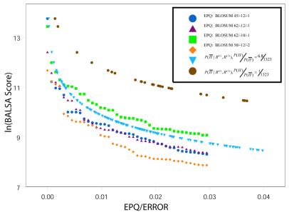
Figure 6 shows the natural log of the BALSA score versus the associated EPQ and posterior probability, P(│ R⁽¹⁾, R⁽²⁾). As shown in Figure 6, P(│ R⁽¹⁾, R⁽²⁾) fits centrally in the individual EPQ graphs for the four scoring matrix and gap penalty combinations. Application of this equation to a database of arbitrary size in which all protein structures are not known requires a prior odds. The specification of this prior generally depends on the application in a manner similar to the selection of a cut-off E()-value. A common and usually conservative assumption is that there is one structural neighbor in the database for each query. Under this assumption the prior odds ratio P(H) / P() becomes 1 / 1323. As shown in Figure 6, this a priori assumption yields a more conservative estimate than the true prior and the EPQ for all parameter combinations.

Figure 6.

The natural log of the BALSA score versus the associated EPQ given the four scoring matrix and gap penalty pairs, P(│ R⁽¹⁾, R⁽²⁾) under the true probability ratio of a homolog versus not, P(H) / P() = 6.8 / 1323, and the a priori assumption P(H) / P() = 1 / 1323. The probability of a non-homolog given the two sequences, P(│ R⁽¹⁾, R⁽²⁾), obtained from the Bayes factor under the true probability ratio is a good estimate of the EPQ independent of the parameters. P(│ R⁽¹⁾, R⁽²⁾) under the a priori assumption is a conservative estimate for the true EPQ and posterior probability obtained from the true prior odds ratio.

Alignment output

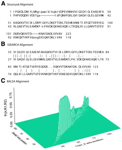
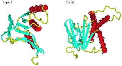
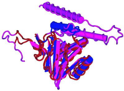
Optimal alignment algorithms return a single alignment, one of an enormous number of possible alignments. For example, the probability of the optimal alignment (see Fig. 9B) obtained with the parameters used by Brenner (1), BLOSUM 45/–12/–1, is 4e–09. The structural alignment (see Fig. 9A) is less likely, 6e–15. Given the parameters used in this analysis, BLOSUM 62/–12/–1, the structural and optimal alignments have probability 1.4e–06 and 6.94e–14, respectively. Instead of a single alignment, BALSA returns the posterior alignment distribution obtained as described in the Backward Recursive Sampling Algorithm. The following example demonstrates how accounting for all alignments in the forward sum can improve coverage. The two proteins depicted in Figure 7 are 1npx_2, NADH peroxidase, and 3lada2, dihydrolipoamide dehydrogenase, with their structural alignment shown in Figure 8. These two proteins are homologs based on structural analysis, but are not reported by SSEARCH, even at large EPQ, but are detected by BALSA as remote homologs. The reason behind this is more clearly seen in Figure 9, the structural and optimal alignments, and the alignment distribution.

Figure 9.

The structural alignment in (A) indicates that nearly all of the alignment between 1npx_2 and 3lada2 is conserved with two gaps. The SSEARCH optimal alignment (B) does not report the alignment of the first 34 residues of inpx_2 and 26 residues of 3lada2 and incorrectly reports the remaining gap. This first section missed is a loop and thus is also missed by the alignment distribution of BALSA (C). The alignment distribution clearly follows a similar pattern to that of the optimal but distinctly shows that there are many alignments similar to the optimal with comparative scores.

Figure 7.

Tertiary structures of 1npx_2 and 3lada2, both multi-domain proteins consisting of multiple α helices and β sheets.

Figure 8.

The structural alignment of NADH peroxidase, 1npx_2, and dihydrolipoamide dehydrogenase, 3lada2.

As indicated earlier, these structural and optimal alignments have extremely low probabilities for both the SSEARCH and BALSA parameters, but there is an interesting comparison between the three alignments. Both BALSA and SSEARCH miss the loop at the beginning of the structural alignment, but if the loop is ignored, then the structural, optimal and distribution alignments begin and end at the same amino acid residues, 35 for 1npx_2 and 27 for 3lada2. The structural and optimal alignments are identical up to residues 65 and 57 for 1npx_2 and 3lada2, respectively. This portion of the alignment has the most sequence identity and is reflected in the BALSA alignment distribution as one large peak. From this point until residues 104 and 95 for the two respective proteins there is only one difference between the structural and optimal alignments, but there is very little sequence identity. This portion of the alignment distribution has many small peaks demonstrating that there are many ways to align this portion with similar probability, but this portion is typically aligned. The most interesting finding comes from the last portion up to residue 120 for 1npx_2 and 111 for 3lada2. The structural and optimal alignments are clearly different and the alignment distribution shows two distinct peaks with significant probability, separating the alignment distribution into optimal- and structural-like alignments. To examine how sums over all alignments may have captured this structural relationship, we drew a sample of 100 000 alignments. Each sampled alignment was directly compared with the structural and optimal alignments by counting the number of aligned pairs in common. The sampled alignment was categorized as structural or optimal, based on which of the two alignments it better matched, yielding 43.9% structural- and 56.1% optimal-like alignments.

DISCUSSION

In this study, we demonstrated how the Bayesian method can be used to address some of the requirements and adjustments associated with the local dynamic programming alignment algorithms. The BALSA algorithm takes into account the uncertainty associated with scoring matrices, gap parameters and alignments by including them all in the joint distribution of the data and the parameters. In our analysis, four score-matrix/gap-penalty pairs were used and in 21.4% of the cases the posterior distribution of the pair deviated considerably from the uniform prior. We also found that no adjustment for length was necessary as there was little relationship between the BALSA score and the sequence length. BALSA outperformed SSEARCH with E()-values on all three databases, increasing coverage from 18.4 to 19.8%, 38 to 41.3%, and 60 to 67.2% at 1% EPQ for PDB40D-B, PDB90D-B and PDB41-90D-B, respectively. The majority of this improvement stems from averaging over all alignments and to a lesser extent from the use of multiple parameter combinations. Additionally, the posterior odds appear to be a useful criterion for assessing the evidence in an alignment of a structural homolog. Figure 9 demonstrates that although portions of the alignment with low sequence similarity give a low score, the summation of all such low-scoring alignments may contribute considerably to the overall score. Additionally, we see here that ∼44% of the sampled alignments are structural like, warranting further investigation into the structural accuracy of the BALSA alignment distribution in comparison with the SSEARCH optimal alignment.

This analysis focused on utilizing Bayesian statistics to address the primary issues of dynamic programming algorithms for local sequence alignment, but it still retains the issue of selecting scoring matrices and gap parameters. This study was restricted to a set of fixed gap/score parameters and methods to overcome this requirement are being examined. Equation 1, L(Θ, Λ) = P(R⁽¹⁾, R⁽²⁾ │ Θ, Λ), is the probability of the data given the parameters and can thus be viewed as the likelihood, yielding a method for obtaining sequence-specific estimatesand. Direct search techniques are being investigated to find these estimates. Additionally, BALSA sums over all possible single subsequence pairs of the two sequences, but does not take into account the possibility of having multiple subsequence pairs between the two sequences. The extension of the local alignment model to take into account multiple local conserved regions in pairwise alignments would yield a super-local alignment procedure.

As is typical of alignment methods, there is a trade-off between speed and accuracy. For comparison of run time on an algorithmic basis it is imperative to use as similar code as possible since code implementation can affect results. Thus, we compared BALSA with the Smith–Waterman algorithm using a minimally modified version of the BALSA code. Given one set of parameters (i.e. a specific set of scoring matrix and gap penalties), the BALSA required 1.3 times more computation time, 13.75 h for BALSA and 10.5 h for Smith–Waterman, on a 1 GHz Pentium III processor for a full all-versus-all comparison of the PDB40D-B database. Given k sets of parameters, BALSA will be slower than SSEARCH by a factor of 1.3k. However, since we found little gain beyond one or two sets of parameters, local Bayesian alignment procedures promise to offer improved potential to identify structural neighbors with little cost in computational requirements.

REFERENCES

- 1.Brenner S., Chothia,C. and Hubbard,T.J.P. (1998) Assessing sequence comparison methods with reliable structurally identified distant evolutionary relationships. Proc. Natl Acad. Sci. USA, 95, 6073–6078. [DOI] [PMC free article] [PubMed] [Google Scholar]
- 2.Pearson W.R. (1995) Comparison of methods for searching protein sequence databases. Protein Sci., 4, 1145–1160. [DOI] [PMC free article] [PubMed] [Google Scholar]
- 3.Smith T.F. and Waterman,M.S. (1981) Identification of common molecular subsequences. J. Mol. Biol., 147, 195–197. [DOI] [PubMed] [Google Scholar]
- 4.Needleman S.B. and Wunsch,C.D. (1970) a general method applicable to the search for similarities in the amino acid sequence of two proteins. J. Mol. Biol., 48, 443–453. [DOI] [PubMed] [Google Scholar]
- 5.Bucher P. and Hofmann,K. (1996) A sequence similarity search algorithm based on a probabilistic interpretation of an alignment scoring system. Proc. Int. Conf. Intell. Syst. Mol. Biol., 44, 44–51. [PubMed] [Google Scholar]
- 6.Sankoff D. (1972) Matching sequences under deletion/insertion constraints. Proc. Natl Acad. Sci. USA, 69, 4–6. [DOI] [PMC free article] [PubMed] [Google Scholar]
- 7.Zhu J., Liu,J.S. and Lawrence,C.E. (1998) Bayesian adaptive sequence alignment algorithms. Bioinformatics, 14, 25–39. [DOI] [PubMed] [Google Scholar]
- 8.Liu J.S. and Lawrence,C.E. (1999) Bayesian inference on biopolymer models. Bioinformatics, 15, 38–52. [DOI] [PubMed] [Google Scholar]
- 9.Gelman A., Carlin,J.B., Stern,H.S., Lyall,A. and Rubin,D.B. (1995) In Chatfield,C. and Zidek,J.V. (eds), Bayesian Data Analysis. Chapman Hall, New York.
- 10.Henikoff S. and Henikoff,J.G. (1992) Amino acid substitution matrices from protein blocks. Proc. Natl Acad. Sci. USA, 89, 10915–10919. [DOI] [PMC free article] [PubMed] [Google Scholar]
- 11.Dayhoff M.E., Eck,R.V. and Park,C.M. (1972) In Foundation,N.B.R. (ed.), Atlas of Protein Sequence and Structure. National Biomedical Research Foundation, Washington, DC, Vol. 5, pp. 89–99.
- 12.Dubin R., Eddy,S., Krogh,A. and Mitchison,G. (1998) Biological Sequence Analysis: Probabilistic Models of Proteins and Nucleic Acids. Cambridge University Press, Cambridge, UK.
- 13.Pearson W.R. and Lipman,D.J. (1988) Improved tools for biological sequence comparison. Proc. Natl Acad. Sci. USA, 85, 2444–2448. [DOI] [PMC free article] [PubMed] [Google Scholar]
- 14.Altschul S.F., Gish,W., Miller,W., Myers,E.W. and Lipman,D.J. (1990) Basic local alignment tool. J. Mol. Biol., 215, 403–410. [DOI] [PubMed] [Google Scholar]
- 15.Brenner S. (1996) Molecular Propinquity. University of Cambridge, Cambridge, UK.
- 16.Karlin S. and Altschul,S.F. (1990) Methods for assessing the statistical significance of molecular sequence features by using general scoring schemes. Proc. Natl Acad. Sci. USA, 87, 2264–2268. [DOI] [PMC free article] [PubMed] [Google Scholar]
- 17.Karlin S. and Altschul,S.F. (1993) Applications and statistics for multiple high-scoring segments in molecular sequences. Proc. Natl Acad. Sci. USA, 90, 5873–5877. [DOI] [PMC free article] [PubMed] [Google Scholar]
- 18.Pearson W.R. (1998) Empirical statistical estimates for sequence similarity searches. J. Mol. Biol., 276, 71–84. [DOI] [PubMed] [Google Scholar]
- 19.Levitt M. and Gerstein,M. (1998) A unified statistical framework for sequence comparison and structure comparison. Proc. Natl Acad. Sci. USA, 95, 5913–5920. [DOI] [PMC free article] [PubMed] [Google Scholar]