Cue: a deep learning framework for structural variant discovery and genotyping

Abstract

Structural variants (SV) are a major driver of genetic diversity and disease in the human genome and their discovery is imperative to advances in precision medicine. Existing SV callers rely on hand-engineered features and heuristics to model SVs, which cannot scale to the vast diversity of SVs nor fully harness the information available in sequencing datasets. Here we propose an extensible deep learning framework, Cue, to call and genotype SVs, which can learn complex SV abstractions directly from the data. At a high level, Cue converts alignments to images that encode SV-informative signals and uses a stacked hourglass convolutional neural network to predict the type, genotype, and genomic locus of the SVs captured in each image. We show that Cue outperforms the state of the art in the detection of several classes of SVs on synthetic and real short-read data and that it can be easily extended to other sequencing platforms while achieving competitive performance.

Introduction

Structural variants (SVs) are the exceptionally diverse set of all genome alterations larger than 50 base pairs. SVs encompass mutations, such as deletions, insertions, inversions, duplications, translocations, and any complex combination thereof, that can reach megabases in size. As a result, SVs account for more base-pair differences across individuals than all other variant types combined [1] and are a key driver of the genetic diversity and disease of the human genome. To date, SVs have been linked to a wide spectrum of disorders, such as cancer, autism, Huntington’s disease, Alzheimer’s, and schizophrenia [2, 3]. Although fundamental to our understanding of human genetics and advances in precision medicine, general SV discovery still remains a largely unsolved problem. This is due both to the limitations of current sequencing technologies, and, more importantly, to the challenges of effectively leveraging all the information available in the data to model and predict SVs in software, while at the same time generalizing to the wide range of SV types and sizes.

Numerous tools have been developed to date to call SVs [4, 5, 6, 7, 8, 9]. These methods typically extract hand-crafted features from the alignment of sequencing data to the reference genome to model both the properties of the sequencing platforms (e.g. molecule lengths and sequencing errors) and the types of SV events (e.g. mapping patterns associated with each type of SV). In whole-genome short-read sequencing, read alignment signals that are commonly used to model SVs include: read depth (the number of reads that map to a genome region), discordant read pairs (pairs of reads from the same fragment whose mapping deviates in distance or orientation from how a contiguous fragment should map), and split reads (reads that have several partial alignments to the reference) [10]. These signals are usually combined into a sophisticated statistical model or a heuristic rule-based pipeline to predict different SV classes and SV breakpoints. As a result, existing tools heavily rely on developer expertise and are tightly coupled to the properties of the sequencing data and the artifacts of preceding analysis steps (e.g. the alignment algorithm). However, given the sheer vastness of the SV landscape and the complexity of SV-informative signals, expert-driven SV detection is inherently intractable, especially for complex SVs, rendering us blind to major classes of genetic drivers of disease.

Deep learning offers the ability to learn complex abstractions directly from large labeled datasets without expert guidance and is hence a promising avenue for general SV discovery. Recently, DeepVariant [11] pioneered the use of deep learning for SNP and small indel calling. At its core, DeepVariant uses a convolutional neural network to classify read pileup images constructed around candidate variant sites into three possible diploid genotypes. This strategy has also been recently applied to the analysis of SVs, primarily for SV genotyping and filtering [12, 13, 14] and deletion detection [15]. However, while a great fit for capturing small events (that can fully fit within some standardized image size), read pileup images are not well suited for detecting complex types and larger sizes of SVs due to the loss of relevant cross-breakpoint information and the added complexity needed to reconstruct one SV call from multiple separate images. Moreover, since SVs are often nested or tightly clustered, and hence multiple SVs can appear in the same image, SV detection cannot be robustly formulated as an image classification task. This motivates the need to develop methodology designed specifically for the problem of general SV discovery using deep learning.

In this work, we propose an extensible framework, Cue, for SV calling and genotyping, which can effectively leverage deep learning to automatically discover the underlying salient features of different SVs, including complex and somatic subclonal SVs. In particular, we formulate SV discovery as a multi-class keypoint localization task, where keypoints correspond to breakpoints of different SV type in multi-channel images. We generate input images for this task by juxtaposing two genome intervals, which can capture both SV breakpoints regardless of SV size, and simultaneously represent multiple read alignment signals as separate image channels. To perform keypoint localization, our approach employs confidence map regression using a stacked hourglass network [16, 17] trained to predict pixels that correspond to SV breakpoints, allowing for multiple clustered SVs of any type to be present in the same image.

To date, we have trained Cue to detect and genotype deletions (DEL), tandem duplications (DUP), inversions (INV), inverted duplications (INVDUP), and inversions flanked by deletions (INVDEL) larger than 5kbp; the latter two are examples of complex SVs, which have been linked to several genomic disorders [8]. To investigate the feasibility of our approach for the analysis of cancer datasets, we have also trained Cue to detect lower-frequency subclonal DELs, DUPs, and INVs. Since high-quality labeled SV callsets in real genomes are still scarce, we have trained our current models entirely on SVs modeled in silico. We show that Cue outperforms state-of-the-art methods in simulation and in the HG002 GIAB benchmark [18]. To further analyze Cue’s performance on real data, we compared its results to short-read and long-read methods on the CHM1 and CHM13 genome mix using short-read Illumina [19] and long-read PacBio [20] datasets. We show that Cue achieved the highest concordance with long-read methods for DELs, while lower concordance was generally observed across technologies for the INV and DUP callsets. Finally, we show a proof-of-concept extension of Cue to long-read and linked-read sequencing platforms. We remark that the variant types, sequencing technologies, and training data we worked with to date are an initial set: our framework can naturally be extended to support more complex variants, additional technologies, and even combinations of technologies, which we will pursue in subsequent framework releases. The implementation of the Cue platform and the pretrained models are freely available under the MIT license at https://github.com/PopicLab/cue.

Results

Overview of the Cue framework.

At a high-level, Cue operates in three steps: (1) read alignments are converted into images that capture multiple alignment signals across two genome intervals, (2) a trained neural network is used to generate Gaussian response confidence maps for each image, which encode the location, type, and genotype of the SVs in this image, and (3) the high-confidence SV predictions are refined and mapped back from image to genome coordinates.

To encode multiple alignment properties, we construct an $n$-channel image from alignments to two genome intervals, where $n$ is the number of extracted alignment signal types. The $x$-axis and $y$-axis of this image correspond to the two genome intervals, such that a pixel maps to some range of base pairs (a locus) in each interval, and the pixel value in each channel encodes the corresponding signal extracted from the reads that map to both pixel loci (see Fig. 1a). Such images capture both the local and long-range genome structure information and can uniquely characterize the type, genotype, and genomic breakpoints of an SV. Note that the pixel corresponding to the start of the SV on the $x$-axis and the end of the SV on the $y$-axis simultaneously encodes both breakpoints (we refer to such pixels as breakpoint keypoints). Therefore, by juxtaposing intervals that are close-by and distant on the genome, we can depict breakpoints of both small and large SVs in the same image. Using a streaming sliding-window approach to scan the genome, we produce candidate genome interval pairs and the corresponding images on the fly.

Fig. 1.

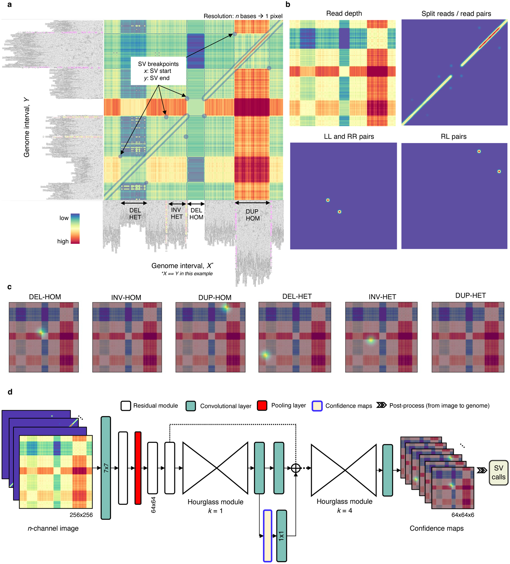
Overview of the Cue framework. a. Conversion of sequence alignments to images. Alignments from a 150kbp synthetic genome interval (visualized in IGV [34]) are shown on the $x$-axis and $y$-axis of the resulting image (displaying the overlay of several signal channels), annotated with four different SVs in this interval. The four highlighted pixel keypoints in the image correspond to the breakpoints of each SV (given by their start coordinate on the $x$-axis and their end coordinate on the $y$-axis). b. SV image channels representing different signals. Given two loci: the read-depth channel shows the difference in depth between the loci; the split-read/read-pairs channel shows the number of split reads or read pairs mapping to both loci; the LL and RR pairs channel shows the number of read pairs mapping in the LL or RR orientation – such pairs are indicative of an inversion; and the RL pairs channel shows the number of read pairs mapping in the RL orientation (where the second read in the pair maps to an earlier position of the reference) – such pairs are indicative of a duplication. c. SV breakpoint confidence maps predicted by the network given the image in A for homozygous (HOM) and heterozygous (HET) DELs, INVs, and DUPs. For simplicity only the read-depth channel is shown as the background. The bright kernels in each map represent a high confidence that the breakpoints of an SV of that specific type and genotype occur at that location, e.g. each pixel in the DEL-HOM map encodes its probability to be a homozygous deletion keypoint. d. The architecture of the stacked hourglass network used in Cue. It takes an $n$-channel image as input and generates a confidence map for each supported SV type and genotype. The predicted confidence maps are then post-processed to produce the final SV callset.

We encode the following alignment signals from short reads: read depth, split reads, read pairs, and the discordant read-pair orientations – namely, left-left (LL), right-right (RR), and right-left (RL). We use different functions to represent these signals (or their combination) in each corresponding channel as described in the Methods section. For example, the read-depth signal is computed as the difference in depth between two loci. Fig. 1b shows several image channels, visualized as heatmaps, generated from read alignments to a genome interval. We stack the resulting channels into an $n$-channel image and use it as input to our deep learning model.

Since the resulting images can contain multiple SVs of different type and size, as well as partially visible SVs, we formulate SV detection as a multi-class keypoint localization task, wherein the objective is to detect the image coordinates corresponding to the two breakpoints of each SV (i.e. the breakpoint keypoints), categorized by SV type and genotype. We solve this task using confidence map regression by training our network to predict a set of confidence maps for each image, such that each map corresponds to an SV type and genotype combination supported by the model (e.g. heterozygous deletion or homozygous inversion) and encodes the location of the breakpoints of all SVs of this type in the input image. Fig. 1c shows the set of six predicted confidence maps, used to detect deletions, inversions, and duplications (split by genotype).

To generate accurate confidence maps, our neural network needs to leverage features at both local and global scale to learn the structural complexity of SV signatures and multi-SV interplay patterns. To this end, Cue uses a fourth-order stacked hourglass convolutional neural network (HN) based on [16, 17], which can consolidate information at multiple scales by repeated bottom-up (pooling) and top-down (upsampling) processing and intermediate supervision. Fig. 1d depicts the high-level network architecture of the HN model used by Cue. The network takes an $n$-channel image as input and outputs a set of confidence maps, encoding the breakpoint keypoints of all SVs in the image. The mean squared error or L2 loss is commonly used to measure the distance between the predicted and the ground truth confidence maps. However, confidence maps encoding a few keypoints using Gaussian kernels mostly consist of background pixels (of value zero), which creates a severe imbalance between foreground and background classes. To address this imbalance, we use focal L2 loss adapted from [21], which allows us to scale down the contribution of easy background and easy foreground pixels when training Cue (see Methods).

Finally, given the confidence maps regressed by the network, we produce the set of output SV calls as follows: (1) we detect all local peaks in each confidence map, (2) refine the keypoint positions, and (3) convert the refined keypoints to genome space to obtain the genome SV breakpoint coordinates. Note that the type and genotype of each SV are directly given by the respective confidence map indices. In addition, non-maximum suppression (NMS) filtering of lower-confidence conflicting calls is performed in both image (2D) and genome (1D) space. Details about each step of the Cue framework are provided in the Methods section.

DEL, DUP, and INV discovery from short-read synthetic data.

To benchmark Cue in single event detection, we simulated a human genome using SURVIVOR [22] based on the GRCh38 reference with a total of 13,504 SVs of size 5–250kbp, with the following breakdown by type: 4,500 DELs, 4,461 tandem DUPs, and 4,543 INVs. Since SURVIVOR places SVs at random positions along the genome, we simulated a large number of SVs, such that some SVs are placed into difficult regions of the genome (e.g. segmental duplications) and clustered near each other.

We compare the performance of Cue in calling and genotyping the simulated events above to four popular state-of-the-art SV callers: Manta [4], LUMPY [6], DELLY [5], and SvABA [7]. Fig. 2a shows the precision, recall, and F1 score of each method at 30x genome coverage computed using the benchmarking tool Truvari [23] (see Supplementary Note 1 for more details on evaluation metrics and Supplementary Notes 4–5 for tool execution details). As shown in Fig. 2a and Extended Data Fig. 1a, Cue consistently achieves the highest scores in the three reported metrics when calling SVs, leading by 1–15% in F1 score and 2–13% in recall. Manta and LUMPY achieve equally high precision across all SV types, with a 2–8% loss in recall. When genotyping SVs, Cue achieves the highest scores in all the metrics on average across all SV types, with a gain in F1 of 5–56%. The biggest increase in F1 score is seen for genotyping DUPs, where Cue leads by 16–45%. On the other hand, Manta and LUMPY outperform Cue by 2–3% in F1 when genotyping INVs, respectively. The Recall-Precision curves in Extended Data Fig. 1b, additionally show the performance profile (i.e. the precision vs recall trade off) of each tool under different SV quality thresholds. To examine the performance of each tool further, Fig. 2b breaks down false negative (FN) calls by size, type, and genome context. We used the RepeatMasker [24] and segmental duplication tracks from the UCSC genome browser [25] to assign SVs to the following four genome context types (as defined in [26]): segmental duplication (SD), simple repeat (SR), repeat masked (RM; all other repeats excluding SD and SR), and unique. We can see that tool performance can vary significantly depending on each SV feature. For example, most tools miss events of smaller size that fall into SD and SR regions of the genome. Cue misses the fewest events in such regions – for example, 195 vs 436 (second lowest) SD events missed by Cue and LUMPY, respectively.

Fig. 2.

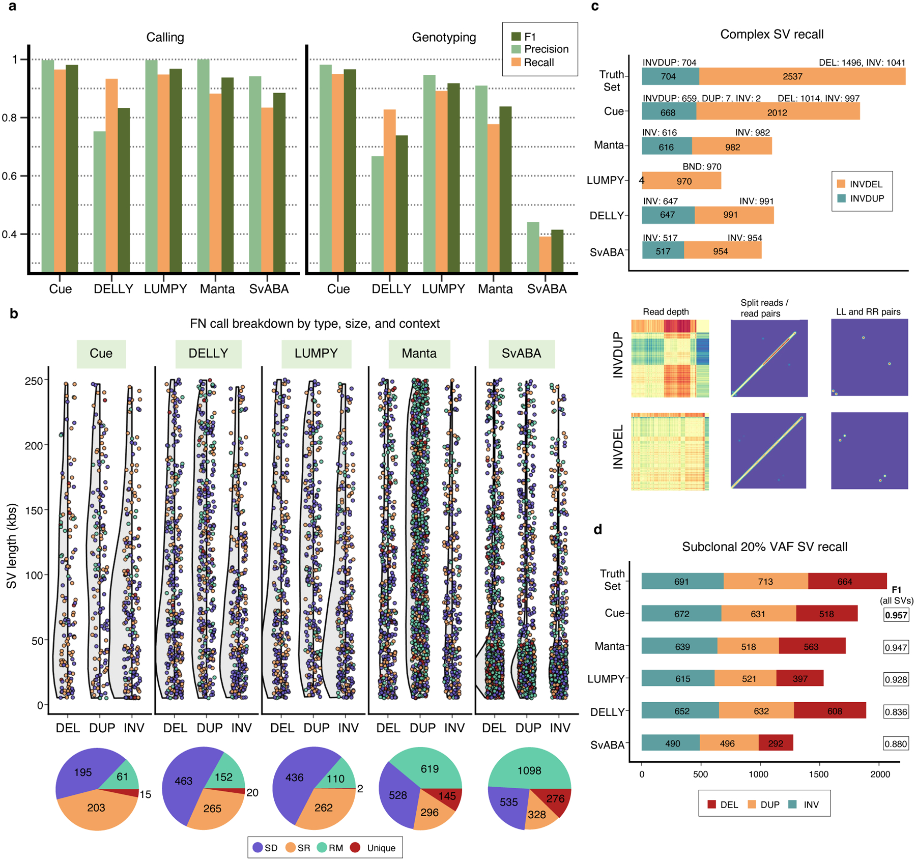
Performance evaluation on synthetic data. a. Precision, recall, and F1 score in DEL, DUP, and INV calling and genotyping at 30x genome coverage. b. FN calls broken down by size, SV type, and genome context. The following number of simulated SVs were assigned to each genome context: SD=1,131(8.3%), SR=786 (5.8%), RM=8,722 (64.6%), and unique=2,865 (21.2%). c. Recall of two complex SV types (INVDUP and INVDEL) at 60x genome coverage. Bottom: Cue image channels for an example of each event type found only by Cue. d. Recall of subclonal somatic SVs broken down by type at 60x genome coverage. All panels: paired-end Illumina short reads were simulated from the corresponding synthetic genome using DWGSIM [35] and mapped with BWA-MEM [36].

Finally, to evaluate Cue’s ability to generalize across sequencing depths, we generated datasets with a coverage of 10x, 15x, 30x, 45x, and 60x for chr1 of this genome. As seen in Extended Data Fig. 2, Cue produces consistently high-accuracy calls (F1 score of 99%) for depths in the range of 15x-60x. At 10x, Cue’s performance drops to an F1 score of 85%. Since the current model was trained only on a mix of high-coverage images (namely, 30x and 60x), a drop in performance at low depths is expected. Cue can be adapted to low-coverage samples by training the model directly on such examples.

Complex SV discovery from short-read synthetic data.

Since our deep learning framework is designed to detect the breakpoints of any number of SVs in the same image, it can be naturally used to detect clustered and complex SVs. To that end, we trained Cue to detect the following two complex SV types: deletion-flanked inversions (INVDEL) and inverted duplications (INVDUP). We represented INVDUPs in Cue as a separate SV type, while detecting INVDELs as three separate SVs (two DELs and one INV). For this benchmark, we simulated a human genome using SURVIVOR with 7,240 SVs of size 5–250kbp in total, of which 1,041 were INVDELs and 704 were INVDUPs. When simulating INVDELs, SURVIVOR chooses the size of the DEL to be a fraction of the size of the INV, resulting in only 1,496 DELs above the 5kbp threshold. We configured Truvari to count a variant as a true positive regardless of its reported type so as not to penalize tools that do not specifically detect or label complex subtypes. Fig. 2c shows the recall of complex SVs broken down by type. Cue discovered a significantly higher number of complex events in this benchmark; in particular, it found 79% of INVDELs, which is >40% greater than the next best result (39% found by DELLY), and 95% of INVDUPs. Of the discovered INVDUPs, Cue labeled over 98.7% events correctly as INVDUPs (with 7 events called as DUPs and 2 events as INV). Manta, SvABA, and DELLY reported all recovered INVDUPs as INVs and LUMPY detected only 4 INVDUP events reported as a DEL, INV, and two breakends (BNDs). For INVDELs, Manta, SvABA, and DELLY did not call any flanking deletions, while LUMPY called all matching events as BNDs. Supplementary Table 1 additionally shows the percentage of recalled variants with a correct genotype for each tool. Cue assigned the correct genotype to >96% of all discovered events. Finally, since Cue reports INVDUPs directly, we could evaluate its precision and found that Cue reports only 1 false positive INVDUP for the entire callset, achieving near-perfect precision for calling INVDUPs in this benchmark.

Subclonal SV discovery from short-read synthetic data.

Somatic SV discovery in cancer genomes is complicated by tumor heterogeneity, wherein some SVs may be present only in certain tumor subclones corresponding to a fraction of the reads in the dataset. As a result, such SVs will have lower variant frequencies (VAFs) and can be challenging to distinguish from noise using manually-designed heuristics. Here we investigate the ability of our method to automatically learn to detect lower VAF subclonal SVs, which will produce fainter signals in our images.

In order to generate WGS data with subclonal SVs, we first simulated two human genome haplotypes using SURVIVOR based on the GRCh38 reference. We then inserted three additional copies of one of the haplotypes and simulated a 60x paired-end short-read dataset from this genome. This resulted in a 20% VAF for SVs from the single-copy haplotype. We used half of the chromosomes of this genome to train Cue, and the other half for evaluation. The evaluation SV callset had a total of 6,266 SVs, with 2,068 subclonal SVs. Fig. 2d shows subclonal SV recall results broken down by SV type, as well as the F1 score achieved by each method on the full evaluation dataset. Cue recovered 97% of all subclonal SVs (96% of deletions, 96% of duplications, and 98% of inversions) while maintaining the highest F1 score. While DELLY recovered the most DEL and DUP events, it also achieved the lowest F1 score (12% lower than Cue) in this benchmark.

HG002 GIAB DEL benchmark.

To evaluate Cue on real data, we used the HG002 genome and its hg19 GIAB NIST Tier1 v.06 benchmarking callset [18] available from the Genome in a Bottle (GIAB) Consortium. This callset contains curated deletion and insertion calls obtained by consensus calling with multiple sequencing technologies; we used only calls from the high-confidence regions provided in this release, which span 2.51 Gbp of the genome. We obtained the 60x Illumina HiSeq reads from GIAB and evaluated Cue and other tools using this dataset. Fig. 3a shows the performance in SV calling obtained by the five methods computed using Truvari for DELs greater than 5kbp (a total of 138 events). In this benchmark, Cue outperformed other methods by 3–22% in F1 score. Manta achieved the highest precision (1% greater than Cue); however, its recall was 10% lower than Cue. On the other hand, LUMPY achieved the highest recall (2% greater than Cue) with a precision drop of 7% compared to Cue. Fig. 3b shows the false negative (FN), false positive (FP), and true positive (TP) DEL calls broken down by size and genome context, and Extended Data Fig. 3a–b show the FN and TP calls broken down by their frequency in the population (computed by matching the HG002 truthset to the gnomAD-SV [27] database using Truvari). The Recall-Precision curves in Extended Data Fig. 3c–d show that Cue achieves a strong balance between precision and recall as compared to other tools. We highlighted several events in Fig. 3b for which IGV plots and Cue-generated image channels are shown in Fig. 3c and Extended Data Fig. 4a–b. In particular: (1) is a TP LINE-1 (L1HS) deletion event detected only by Cue, (2) is a FP event called by DELLY, LUMPY, and Manta, and not called by Cue, and (3) is a FP event called by DELLY, LUMPY, Manta, and SvABA, and not called by Cue. We found that the mapping signature observed for the FP events (2) and (3), along with several variations, is commonly reported as a DEL by short-read SV callers. However, additional properties of this mapping signature reveal that it is often the result of either a dispersed DUP or a divergent reference repeat (defined as the presence of two inexact copies of a locus in the reference sequence) as illustrated in Extended Data Fig. 5. An in-depth analysis at the breakpoints of events (2) and (3) using PacBio CCS reads obtained from GIAB revealed event(2) to be a divergent repeat in the reference (see Supplementary Note 2), while event (3) to be induced by two dispersed DUPs and one inverted dispersed DUP (Extended Data Fig. 4c). Since Cue leverages the information across all the channels jointly, it makes accurate predictions for these events.

Fig. 3.

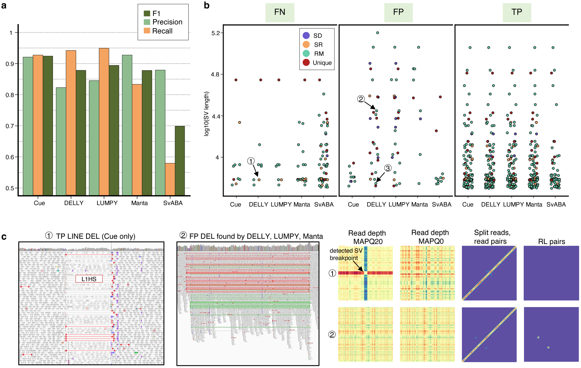
Performance evaluation on the HG002 GIAB DEL benchmark. a. Precision, recall, and F1 score in DEL calling. b. FN, FP, and TP calls broken down by size and genome context. (1)-(3) are FN and FP SV calls analyzed in panel c and Extended Data Fig. 4. c. IGV plots and Cue image channels for (1) TP LINE-1 deletion event detected only by Cue and (2) FP deletion call made by DELLY, LUMPY, and Manta. IGV shows RL read-pair alignments in green and read pairs with a discordantly large insert size in red. As we can see in the Cue-generated channels, the LINE-1 deletion signature of event (1) is well-captured in the high-MAPQ read-depth channel (which shows the drop in coverage consistent with a deletion or a repeat) and the split-read/read-pair channel (which shows the novel adjacency formed by discordant read pairs). The signatures in these two channels jointly, along with the absence of signal in the remaining channels, can uniquely characterize a deletion of a repeat element. On the other hand, while the split-read/read-pair channel alone at the site of FP event (2) can be consistent with a deletion, the presence of the RL signal and the absence of read-depth signal are not jointly consistent with a deletion. Long-read analysis found this event to be a divergent repeat as described in Extended Data Fig. 5 and Supplementary Note 2.

CHM1 and CHM13 diploid mix benchmark.

We further evaluated Cue using the haploid hydatidiform mole CHM1 and CHM13 cell line samples. We obtained the 40x Illumina WGS reads for each sample, merged the reads to create a diploid 80x mix in silico, and mapped the resulting dataset against the GRCh38 reference using BWA-MEM. Since a high-confidence truthset is not available for these two genomes, we used three callsets derived from PacBio CLR long reads for orthogonal validation. In particular, we used the published Huddleston et al. callset [20], along with Sniffles [8] and PBSV [9] calls obtained from the PacBio CHM1 and CHM13 long reads published by [20]. Fig. 4a is an upset plot depicting the agreement across all evaluated callsets for DEL events larger than 5kbp. Tool callset overlaps were computed using SURVIVOR (see the Supplementary Note 1 for details). All callers discovered the same 80 DEL events, with an additional 33 events found by everyone except SvABA. Of the short-read callers, DELLY and LUMPY produced the largest set of unique calls (264 and 105, respectively). Cue has produced 20 unique calls and Manta has produced only 9 unique calls. Since these events are likely to be FPs, we can estimate that DELLY and Manta achieved the lowest and highest precision, respectively, which is consistent with the HG002 benchmark. Next we looked at how many short-read calls were found by at least one long-read caller. As seen in Fig. 4b, the significant majority of Cue calls (172 out of 195) were found by at least one long-read method – the largest fraction of calls of all short-read methods. Supplementary Fig. 1 shows an example of a true LINE-1 DEL event found only by Cue and all the long-read methods. Next we manually examined the groups of events found by multiple short-read callers only. For example, 42 events were reported by all short-read callers except Cue. Even though tool consensus is high for these events, we found that a large fraction of them are likely FP calls caused by a dispersed DUP or a divergent repeat in the reference, similar to FP DEL calls found in HG002. For example, 12 of the 42 events had a DUP call reported by at least one of the four methods at the same locus. Fig 4c shows the IGV plots of two such DEL calls that are consistent with a divergent reference repeat. Examining the methodology and the reported SV evidence of each method, we found that the tools relied solely on the discordant read-pair signal to call these DELs. Although each method can use additional sources of evidence, no tool requires the concordance of multiple distinct evidence sources to make a call nor takes into account the presence of any conflicting evidence (e.g. the RL signal or the lack of change in read depth). This points to the difficulty of hand-engineering a model that can combine multiple, potentially discrepant, sources of evidence at the same location. Therefore, since existing short-read tools can call events using the same underlying assumption, their consensus often cannot be considered as a validation of shared events.

Fig. 4.

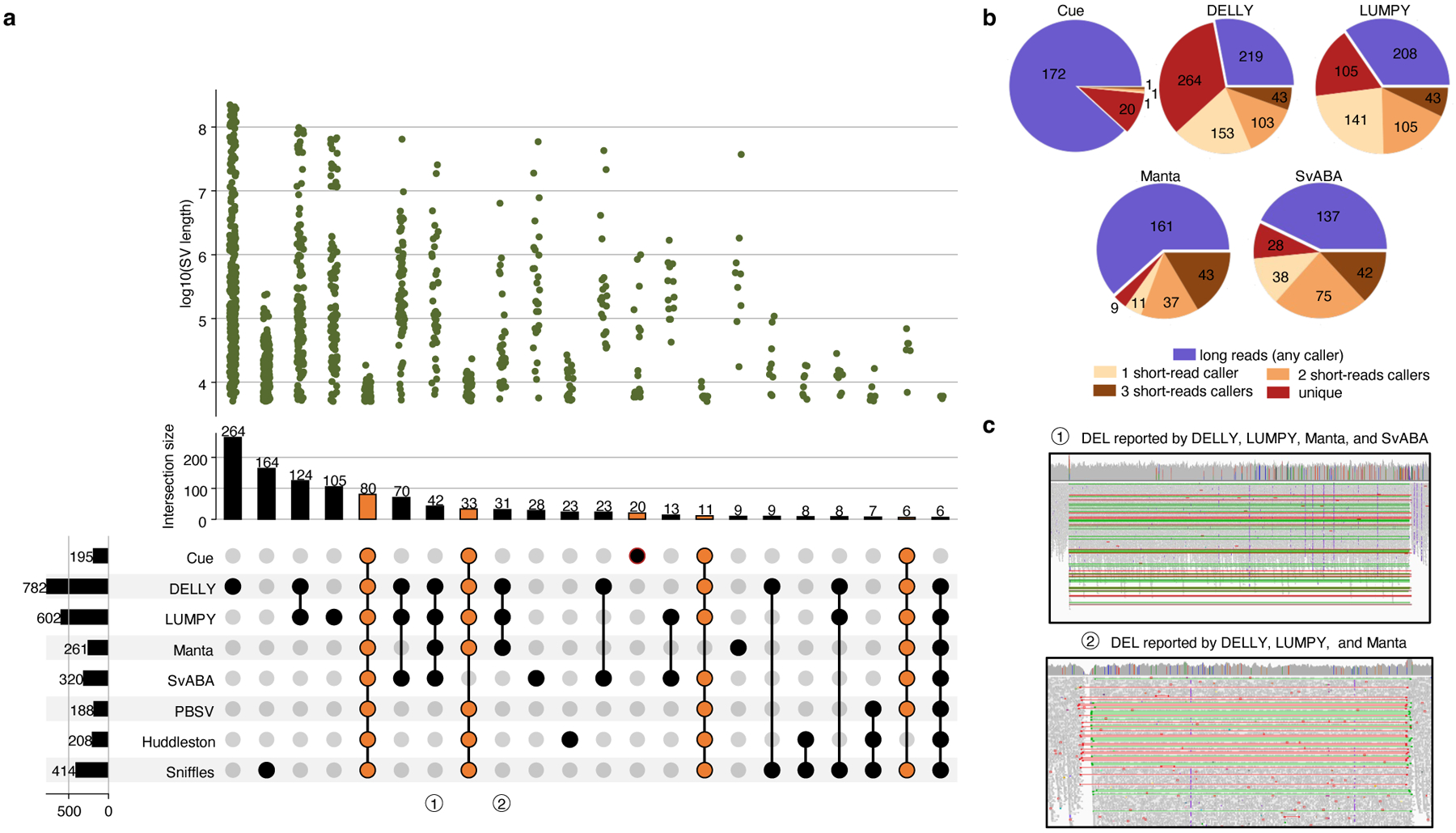
Performance evaluation of DEL calling on the CHM1+CHM13 benchmark. a. Upset plot depicting DEL callset overlaps of five short-read and three long-read callers (only sets larger than 5 events are displayed for conciseness). Overlaps that include Cue are highlighted in orange. b. Breakdown of DEL calls by consensus with long-read and short-read callers. c. IGV plots of (1) a DEL reported by all short-read callers except Cue and (2) a DEL reported by DELLY, LUMPY, and SvABA that are consistent with a divergent reference repeat.

We performed a similar analysis for DUP and INV events reported in Extended Data Fig. 6. As opposed to the DEL benchmark, the consensus across callers is considerably smaller for these event types. In particular, only one DUP and zero INVs were reported by all of the short and long-read callers. A considerable number of DUP events (namely, 42) were reported by all short-read callers except Cue. Since consensus for these calls was high, we manually examined them individually. We found that 18 out of the 42 events were found within centromeric satellite repeat regions, which are notoriously difficult to analyze using short reads. As shown in Supplementary Fig. 2, existing methods produce numerous overlapping DUP calls in such regions due to the abundance of RL pairs. Of the remaining calls, we found that 17 were also reported as DELs by some of the tools and were consistent with dispersed DUP or divergent repeat signatures. Overall these results point to the difficulty of calling DUPs and INVs using existing methods, and using orthogonal technologies for validation. More importantly, they reveal the need for a benchmarking dataset for such events (and especially complex SVs) that can be used to evaluate existing and future tools.

DEL, DUP, and INV discovery in the presence of decoy events.

Given the results on real data, where the presence of complex events (e.g. dispersed DUPs) often confounded the detection of single DEL, DUP, and INV events, we created a synthetic benchmark to investigate the performance of each tool in detecting these single events in the presence of other decoy events in the genome. In particular, we simulated a synthetic genome with 1,000 DELs, 1,000 DUPs, and 1,000 INVs in the range of 5–250kbp, as well as 1,000 translocations (TRAs), 1,000 dispersed duplications (dDUPs), and 1,000 inverted dispersed duplications (inv-dDUPs) to serve as decoys. We then simulated a 60x paired-end short-read dataset from this genome. Fig. 5a shows the IGV plots of the six types of simulated events. It can be seen that certain types of read-pair signals are shared across these event types; however, each event type corresponds to a unique combination of signals. Fig. 5b shows the precision, recall, and F1 scores of each method in DEL, DUP, and INV calling. While the recall of each method is still high, precision is significantly affected by the presence of decoy events that partially share paired-end evidence with DELs, DUPs, and INVs. Cue achieves substantially higher results in each metric in DEL and DUP calling in this benchmark, leading by 52–55% and 57–63% in precision, 4–13% and 2–10% in recall, and 45–49% and 41–48% in F1 score, respectively. In INV calling, LUMPY achieves the highest F1 score of 98%, with Cue achieving the second highest score of 93%, followed by Manta at 66%. This experiment shows that Cue is able to learn complex representations for simple SV types that automatically capture and reconcile multiple types of SV-informative signals.

Fig. 5.

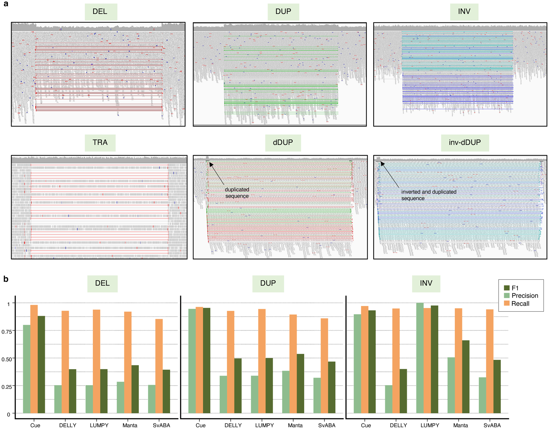
Performance evaluation on synthetic data in the presence of decoy events. a. IGV plots of DEL, DUP, INV, TRA, dDUP, and inv-dDUP events. b. Precision, recall, and F1 scores in DEL, DUP, and INV calling.

Extending Cue to long and linked read sequencing platforms.

To demonstrate that our approach can be extended to different sequencing platforms, we have also performed a preliminary evaluation of Cue on long-read and linked-read data. Fig. 6a and Supplementary Note 3 describe the inputs constructed for these platforms. We used the same synthetic genomes for evaluation and training and simulated long reads at 30x coverage using PBSIM2 [28] (aligned with minimap2 [29]) and linked reads at 60x coverage using LRSIM [30] (aligned with Longranger [31]).

Fig. 6.

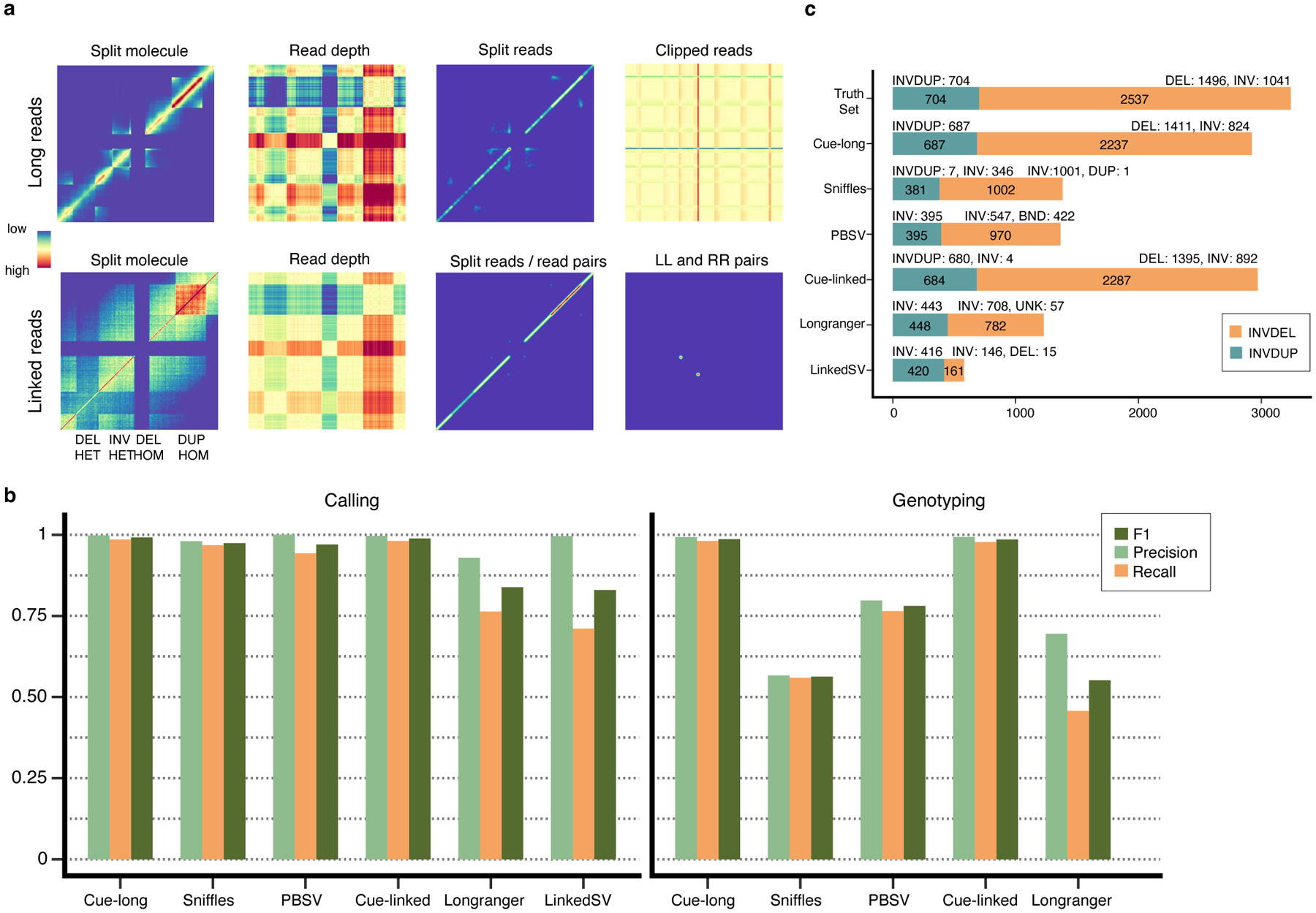
Extending Cue to long and linked read sequencing platforms. a. Image channels generated from synthetic PacBio CLR long reads and 10x Genomics linked reads, computed for an interval of the genome containing four different SVs (labeled along the $x$-axis; the same interval is assigned to both axes). b. Precision, recall, and F1 score in DEL, DUP, and INV calling and genotyping. LinkedSV does not output SV genotypes and is omitted. c. Recall of two complex SV types (INVDUP and INVDEL) using long and linked reads.

We compared the performance of Cue to state-of-the-art long-read SV callers, PBSV [9] and Sniffles [8], and to linked-read SV callers, Longranger [31] and LinkedSV [32]. We performed the evaluation on the two synthetic benchmarks described above for single-event (DEL, INV, and DUP) and complex-event (INVDUP and INVDEL) discovery. As shown in Fig. 6b, Cue achieved the highest scores in DEL, INV, and DUP calling. We see the biggest performance gap in comparison to linked-read methods, where Cue leads by 15% in F1 score. Note that state-of-the-art linked-read callers are also outperformed by existing short-read callers, suggesting that developing expert-driven software that fully leverages linked-read signals is particularly difficult. Cue achieves significantly higher genotyping accuracy with both long and linked reads as well.

Fig. 6c shows the recall of complex SVs broken down by type. As with short reads, Cue discovered a significantly higher number of complex events in this benchmark. In particular, it found 98% and 97% of INVDUPs using long reads and linked reads, respectively, while only 56% and 64% of these events were found by the leading tools, PBSV and Longranger, respectively. Cue labeled 100% of the detected events correctly as INVDUPs using long reads and 99% using linked reads. Existing methods reported most of the recovered INVDUPs as INVs. Only Sniffles was designed to detect INVDUPs specifically; however, of the recalled 381 (54%) SVs, it reported only 7 as actual INVDUPs, and the majority as INVs. Furthermore, Cue found 88% (with long reads) and 90% (with linked reads) of INVDELs, respectively, which is significantly greater than the next best result of 39% found by Sniffles. For INVDELs, existing methods missed most of the flanking deletions and discovered only a fraction of the inversions.

In conclusion, by applying modifications only to the image channels, our approach can be extended to other sequencing platforms, while matching or surpassing state-of-the-art methods that were manually tailored to those platforms. This combination of power and simplicity of deployment allows Cue to keep up with the rapid advances in sequencing technology and to deliver optimal performance on each platform.

Discussion

In this work we motivate the use of deep learning for structural variant discovery, which allows us to shift method development away from ad hoc hand-engineered pipelines to scalable and sustainable models that can learn complex patterns of variation directly from the data. We lay out how SV detection can be formulated as a deep learning computer vision task and propose an extensible framework, Cue, to call and genotype SVs of diverse size and type. We demonstrate state-of-the-art results in calling several SV classes from synthetic and real short-read datasets. For a proof of concept, we show how Cue can be adapted to PacBio CLR long reads and 10x Genomics linked reads and achieve state-of-the-art performance, especially in complex SV discovery. We will expand the framework in future work to formally support these additional sequencing platforms, a larger range of SV sizes (which can be achieved by changing the basepair-to-pixel resolution of our images), and more SV types (such as translocations, insertions, and other complex SVs).

A major requirement and challenge for data-driven SV discovery is the availability of large and well-balanced training datasets. While numerous callsets are available in publicly-available repositories, such as GIAB and HGSVC [33], high-confidence calls that can be used reliably for training are currently very scarce. To compensate for the lack of labeled real genomes, we have used in silico SV modeling for training. This approach can produce arbitrarily large well-balanced datasets; however, extensive modeling is required to capture the full repertoire of sequencing technology characteristics, SV types, and genome contexts observed in real data. We expect the model to struggle with event types it has never seen during training; therefore, including real data into the training dataset is critical both for performance and generalizability. To that end, we will retrain our model as our SV truthsets grow over time, while leaving our core framework untouched.

Methods

Multi-channel image generation.

Given a set of read alignments $A$ from an input BAM or CRAM file, a set of candidate genome interval pairs $G$ (with intervals of size $S$), and a set of $n$ predefined alignment signal scalar valued functions $F=\left\{f^1,f^2,\dots ,f^n\right\}$ (where $f^k:A\times {\mathbb{R}}^2\to \mathbb{R}$) mapping alignments extracted from two regions of the genome to a single value, we create an $n$-channel $w\times h$ image for each interval pair $\left(g_x,g_y\right)\in G$, where the $k$th image channel is obtained as follows. First we use the function $f^k\in F$ to compute a square matrix ${\mathbf{M}}^k$, such that ${\mathbf{M}}_{ij}^k=f^k(A,i,j)$. The dimension of ${\mathbf{M}}^k$ is $\frac{S}{B}\times \frac{S}{B}$, where $B$ represents the matrix resolution (or the number of genome base pairs that correspond to one entry in $\mathbf{M}$). The $i^{\text{th}}$ row in ${\mathbf{M}}^k$ corresponds to the genome region (or bin) $g_y[iB\dots (i+1\left)B\right)$, the $j^{th}$ column corresponds to the genome region $g_x[jB\dots (j+1\left)B\right)$, and the value ${\mathbf{M}}_{ij}^k$ is given by applying $f^k$ to alignments in regions $i$ and $j$ (denoted as the alignment subsets $A^i$ and $A^j$, respectively). We assign an alignment to a region if its midpoint position falls into the region. Post-construction, each matrix is down-sampled (using block summation) or up-sampled (using nearest neighbours) to size $w\times h$, depending on the configured values of $S,B,w$, and $h$, and its values are normalized to fall in the range [0, 1]. In the resulting image, genome positions from the interval $g_x$ are on the $x$-axis and those from $g_y$ are on the $y$-axis, respectively. Presented results were obtained with images of size $256\times 256$ pixels, $B$ of 750bp for SV discovery and $B$ of 200bp for SV refinement, and $S$ of 150kbp.

We define the following alignment signal functions (note: we denote the sets of a specific property taken from all elements in a given alignment set using subscript notation; for example, the set of all read names taken from the alignments in a subset $A^i$ is given by $A_{\mathit{\text{name}}}^i$.):

• The read-depth function

  $$\left|A^i\right|-\left|A^j\right|$$

  computes the difference in coverage in regions $i$ and $j$ normalized such that negative values fall in the range [0, 0.5), and positive values fall in the range (0.5, 1] (to distinguish between deletion and duplication events); we compute two channels using this function with (1) only MAPQ>20 alignments and (2) all alignments (including MAPQ=0).
• The split-read and read-pair function

  $$\left|A_{\mathit{\text{name}}}^i\cap A_{\mathit{\text{name}}}^j\right|$$

  computes the number of reads or read pairs mapping to both bin $i$ and $j$, where read pairs and split-read alignments are given the same name.
• The read-pair $\text{LL}$ and $\text{RR}$ orientation function

  $$\left|A_{\mathit{\text{name}},\{LL,RR\}}^i\cap A_{\mathit{\text{name}},\{LL,RR\}}^j\right|$$

  computes the number of read pairs that map to both bin $i$ and $j$ in the same orientation; these mappings are common with inversions.
• The read-pair $\text{RL}$ orientation function

  $$\left|A_{\mathit{\text{name}},RL}^i\cap A_{\mathit{\text{name}},RL}^j\right|$$

  computes the number of read pairs that map to both bin $i$ and $j$ in the RL orientation, where the second read in the pair maps to an earlier position on the reference; these mappings are common with duplications.
• The read-pair orientation ratio function

  $$\frac{\left|A_{\mathit{\text{name}}\{LL,RR\}}^i\cap A_{\mathit{\text{name}},\{LL,RR\}}^j\right|}{\text{min}\left(\left|A^i\right|,\left|A^j\right|\right)}$$

  computes the ratio in coverage by $\text{LL}$ and $\text{RR}$ read pairs versus read depth, which is indicative of the inversion genotype.

In order to boost the signal from discordant mappings, the normalized output of the read-pair orientation functions is also passed through a dilating maximum filter and a Gaussian filter.

To speed up computation, we build, in a single pass over the input BAM file, an index that allows us to quickly query several properties of the alignments mapped to individual genome bins. More specifically, we partition each chromosome into $B$-sized bins, and store the following sets of values extracted from the reads assigned to each bin: (1) number of $\mathit{\text{MAPQ}}\ge 20$ reads, (2) number of all reads, (3) read names, (4) read names of the $\text{LL}$ and $\text{RR}$ read-pairs, (5) reads names of the RL read-pairs. Each function can then be easily computed via index lookups (e.g. the split-read and read-pair function can be computed as the intersection of the read names stored in the corresponding two bins of the index). All images are generated on-the-fly in small batches in memory as we scan the genome and deallocated immediately after use (images are not pre-generated or stored on disk). The batch size is a configurable parameter that can be tuned to achieve the desired tradeoff of throughput and RAM consumption (e.g. larger batches can increase the GPU inference throughput while also increasing the memory consumption).

Interval pair selection.

We use the following strategy to generate $G$, the set of candidate interval pairs (for which images are constructed) that capture both small and large SV events on each chromosome. Let $L$ be the length of a chromosome sequence and $K$ be the step size of the sliding window. Then, for a given interval size $S$, we produce the set of interval pairs $G\in g\times g$ where $g=\left\{\right[x,x+S)\mid x=Kp,\forall p\in [0,(L-S)/K\left]\right\}$ is the set of all intervals of size $S$ that start at every $K^{th}$ position on the chromosome. We only add interval pairs $\left(g_x,g_y\right)$ to $G$ that have at least two discordant read pairs, such that one alignment of the read pair is contained in $g_x$ and the other alignment is contained in $g_y$, for every $g_x$ and $g_y$ in $g$. In our experiments, we set $K=50\mathrm{k}\mathrm{b}\mathrm{p}$ and $S=150\mathrm{k}\mathrm{b}\mathrm{p}$. We can find smaller events by reducing the size of the intervals, $S$, to enlarge them in the image. The number of interval pairs generated in our benchmarks was 61,296 for the $30x$ synthetic genome, 16,850 for HG002, and 30,119 for the CHM-mix dataset, respectively.

SV confidence map regression.

Given an $n$-channel image $I$ generated for the genome interval pair $\left(g_x,g_y\right)$, our neural network outputs a set of confidence maps $H=\left\{h_1,h_2,\dots ,h_T\right\}$ corresponding to the $T$ zygosity-aware SV types supported by the model. Each confidence map encodes the predicted location of the breakpoints of all the SVs of a particular type in the input. More specifically, let $\left(b_x,b_y\right)$ be the coordinates of a given SV’s breakpoints in the genome (i.e. its start and end positions). If $b_x\in g_x$ and $b_y\in g_y$, we can map these breakpoints to a keypoint $\mathbf{p}=\left(\frac{\left(b_x-g_x^{\mathit{\text{start}}}\right)}{B},\frac{\left(g_y^{\mathit{\text{end}}}-b_y\right)}{B}\right)$ in $I$. If detected, this keypoint is sufficient to infer the genome coordinates of this SV within $B$ base pairs by mapping its pixel coordinates back to genome space. Visually, the SV keypoint corresponds to the top-left corner of the square defined by the start and end coordinates of the SV on each axis of $I$.

We generate ground-truth confidence maps of size $w^H\times h^H$ to train the network as follows. For each SV, $v$ (provided as a ground-truth BED or VCF file), overlapping $g_x$ and $g_y$ with a visible keypoint ${\mathbf{p}}^v$ (i.e. $b_x^v\in g_x$ and $b_y^v\in g_y$), we add an unnormalized 2D Gaussian distribution peak centered around ${\mathbf{p}}^v$ to $h_t$, where $t$ represents the type of the SV. As a result, for each SV type $t\in \{1\dots T\}$, the values at $\mathbf{x}\in {\mathbb{R}}^{w^H\times h^H}$ in $h_t$ are given by

$$h_t(x)=\sum _{v\in V_t}\text{exp}\left(-\frac{{\Vert x-p^v\Vert }_2^2}{2{\sigma }^2}\right)$$

where $V_t$ is the set of all SVs in $I$ of type $t$. The hyperparameter $\sigma$ of the Gaussian kernel determines the spread of each keypoint peak and can be used to balance the ratio of foreground and background pixels. The confidence map size is determined by the stride hyperparameter $s$, which controls the ratio between the input image size and the confidence map size. In our experiments we generate confidence maps of size $64\times 64$, given by $s=4$ (with $\sigma =10$).

Network structure and training.

Our deep learning model is a fourth-order stacked hourglass network based on the human pose estimation model proposed in [37, 38]. The network starts with a convolutional backbone module through which the image is fed prior to the four hourglass modules. The backbone consists of a $7\times 7$ convolutional layer, a residual module, a max-pooling layer, and two additional residual modules. For input images of size $256\times 256$, the backbone reduces the resolution down to $64\times 64$ (our confidence map size). Each hourglass module consists of residual modules and max pooling layers to process the input features down to a low resolution, followed by nearest neighbor upsampling layers and skip connections to get back up to the output resolution. We perform intermediate supervision after each hourglass module, resulting in each hourglass module generating its own set of intermediate confidence map predictions from which we compute a loss. Stacking and intermediate supervision allow the network to repeatedly reassess its estimates and features at every scale. For more details on the HN architecture, please see [37, 38].

Our network was implemented in Pytorch. To train the network we used the Adam optimizer [39], a learning rate of $1e^{-4}$, and a batch size of 16. We used a random subset of our training dataset (10% of the data) as a heldout validation set to evaluate the model during training.

Focal loss.

We use focal L2 loss adapted from [40] to compute the distance between the predicted and the ground truth confidence maps. Let $h_t^k$ be the predicted confidence map of size $w^H\times h^H$ for SV type $t$ by hourglass module $k$ and let $h_t^G$ be the ground truth confidence map for this SV type, the focal L2 loss between these two confidence maps is defined as follows:

$$F{L}_t^k=\sum _{p\in {ℝ}^{w^H\times h^H}}{\Vert h_t^k(p)-h_t^G(p)\Vert }_2^2\cdot {\Vert 1-D_t^k(p)\Vert }_2^2,\text{ where }{D}_t^k(p)=\{\begin{array}{ll}{h}_t^k(p)-\alpha ,\hfill & h_t^G(p)>\theta ,\hfill \\ 1-h_t^k(p)-\beta ,\hfill & \text{otherwise}\hfill \end{array}$$

The hyperparameter $\theta$ is the threshold used to separate background and foreground pixels, while $\alpha$ and $\beta$ are used to scale down the contribution of easy background and easy foreground pixels. The total loss for the stacked HN, summed over the four stacked hourglass modules and SV types, is then computed as:

$$FL=\sum _{k=1}^4\sum _{t=1}^{T}F{L}_t^k$$

Converting regressed confidence maps to final SV calls.

Since the input images can contain multiple SVs of the same type, we detect all local maxima in each regressed confidence map using a maximum filter and thresholding (i.e. only values above a certain threshold are kept as candidates; we use 0.4 as the threshold in our experiments). Given the resulting set of peak keypoints, we perform 2D non-maximum suppression (NMS) by finding the SV breakpoint bounding boxes defined by each keypoint and filtering keypoints with conflicting or redundant bounding boxes. More specifically, let $(x,y)$ be the coordinates of a candidate SV keypoint. The bounding box defined by this SV’s breakpoints is given by the following confidence map coordinates: $\left.\left[x_{min}=\right. x,y_{\mathrm{m}\mathrm{i}\mathrm{n}}=y,x_{\mathrm{m}\mathrm{a}\mathrm{x}}=w-x,y_{\mathrm{m}\mathrm{a}\mathrm{x}}=h-x\right]$. For each pair of resulting bounding boxes $(M,N)$, we compute the intersection over union, $IoU=|M\cap N|/|M\cup N|$ and intersection over minimum, $IoM=|M\cap N|/\mathrm{m}\mathrm{i}\mathrm{n}\left(\right|M|,|N\left|\right)$, metrics and remove the keypoint with the lower score if the $IoU$ or $IoM$ values are above a specified threshold (i.e. the boxes have substantial overlap).

In order to increase the accuracy of Cue’s breakpoint positions, we optionally refine the location of the remaining keypoints using higher resolution images “zoomed-in” around SV keypoints. During refinement, we extract a small patch of the initial image around each predicted keypoint and pass the patch through our model to obtain a higher resolution keypoint. To minimize the number of base pairs represented by each pixel, the input images are constructed using a smaller genome bin size $\left(B\right)$, resulting in higher resolution.

Each refined SV keypoint coordinate $(x,y)$ is then converted to genome breakpoint coordinates, with the $x$ coordinate giving the start position of the SV and the $y$ coordinate giving its end position (as previously described). Since each confidence map encodes only keypoints of SVs with a specific type (and genotype), we can directly determine the type and genotype of each SV call based on the index of the confidence map in which it was detected.

The above process produces a set of SV calls for each image, which are then collected and filtered using 1D NMS, wherein we compute the $IoU$ and $IoM$ metrics for the SV intervals on the genome to find and filter out near-duplicate or conflicting SVs. Since multiple images can capture the same part of the genome, and hence call the same SV, we need this step to remove such duplicate calls. Finally, our method can also be configured to filter out SVs falling into blacklisted regions of the genome (e.g. assembly gaps); however, this is not enabled by default.

Training data generation.

To generate training data for our model, we simulated a human genome using SURVIVOR with 13,864 SVs of size 5–250kbps, consisting of homozygous and heterozygous deletions, tandem duplications, inversions, deletion-flanked inversions, inverted duplications, insertions, and translocations (note: insertions and translocations were included in the simulated genome but not labeled for training in the images). When simulating SVs, SURVIVOR selects the size, the zygosity, and the genome location of each SV at random. Additionally, we added small insertions and deletions (of size 50bp - 1kbp). Since SURVIVOR chooses genome positions at random, we have simulated a large number of SVs within the same genome, to guarantee that SVs are placed in a variety of genome sequence contexts and co-occur nearby on the genome in different combinations. This procedure resulted in the following breakdown of SVs by sequence context in our labeled training examples: 1,101(8%) in segmental duplications; 913 (7%) in simple repeats; 9,190 (66%) in all other repeat types; and 2,660 (19%) in non-repetitive regions. We generated a 60x paired-end Illumina short-read WGS dataset from this genome using DWGSIM and mapped the reads with BWA-MEM to obtain a BAM file with read alignments.

Given the generated BAM file and the ground-truth SV BED file produced by SURVIVOR, we generated an annotated training image dataset by: (1) scanning the genome using a sliding-window approach to produce genome interval pairs, (2) generating images from the alignments to each interval pair, and (3) annotating the resulting images with information that includes the SV type and breakpoint coordinates of each visible (or partially visible) SV, as well as genome intervals used to generate the image. This scheme resulted in 175,934 images with 0–6 SVs fully visible in the same image. To diversify the genome coverage of our training examples, we have also down-sampled the generated BAM file to a depth of 30x and generated new images for this depth. In addition, we have also augmented SURVIVOR to model LINE-1 deletions by selecting random LINE-1 breakpoints from the LINE track of RepeatMasker, and simulated 7,501 such events with 51,541 corresponding images. Finally, we also generated 48,073 image examples using reads simulated directly from the reference genome, 10,400 images with divergent read alignments (to model divergence, we simply down-sampled reference-read alignments at random loci of the genome), and 193,361 images with unlabeled dispersed duplications and inverted dispersed duplications. Extended Data Fig. 7 shows a high-level diagram of the in-silico training data generation process and a sample of produced annotated images.

Runtime and memory requirements.

We evaluated the runtime and memory requirements of Cue on the 60x HG002 genome and compared its performance to the four state-of-the-art short-read callers. All our experiments were performed on an Intel Xeon Gold 6258R system with 56 physical cores and maximum single-core frequency of 4GHz, four NVIDIA RTX A6000 GPUs, and 2TB of RAM. For each experiment, we report the average wall clock time and the average maximum resident set size (Max RSS) over five executions of each program.

To evaluate single-core performance, we first executed each method on chr1 of the HG002 genome configuring each tool to run on a single thread. As can be seen in Extended Data Fig. 8a–b, Cue required 5.6GB of peak memory and 1h runtime on this benchmark (of which 20min was spent in indexing the BAM file and 42min in SV calling). SvABA ran slightly longer than Cue and DELLY required slightly more RAM. When configuring PyTorch to use multiple CPUs or a single GPU, the calling time of Cue was reduced to 20min on chr1 (Extended Data Fig. 8c).

Next we evaluated the runtime of Cue on the full HG002 genome. Cue can be configured to process each chromosome in parallel across multiple CPUs or a single or multiple GPUs. When running on 24 CPU cores in parallel (such that each chromosome is assigned to a separate core), Cue processed the full genome in 40min (when pre-indexed) and 1h from scratch, with a Max RSS of 37GB. This runtime is dominated by the time it takes one core to process chr1. Enabling parallel processing in PyTorch (which runs inference on multiple images of the same chromosome in parallel), brings the SV calling time down to 30min. Using a single GPU (filled to capacity with 18 chromosomes processed in parallel and a batch size of 16), reduces the runtime further down to 20min. Using all four GPUs (by assigning each GPU to 6 chromosomes) did not reduce runtime significantly for any batch size. Since Cue was implemented in Python, we expect that a significant increase in performance can be achieved by shifting the index computation to C++. Furthermore, we plan to optimize SV calling and index construction in future releases, by performing a fine-grained load-balanced assignment of interval pairs (rather than chromosomes) to parallel threads.

Extended Data

Extended Data Fig. 1.

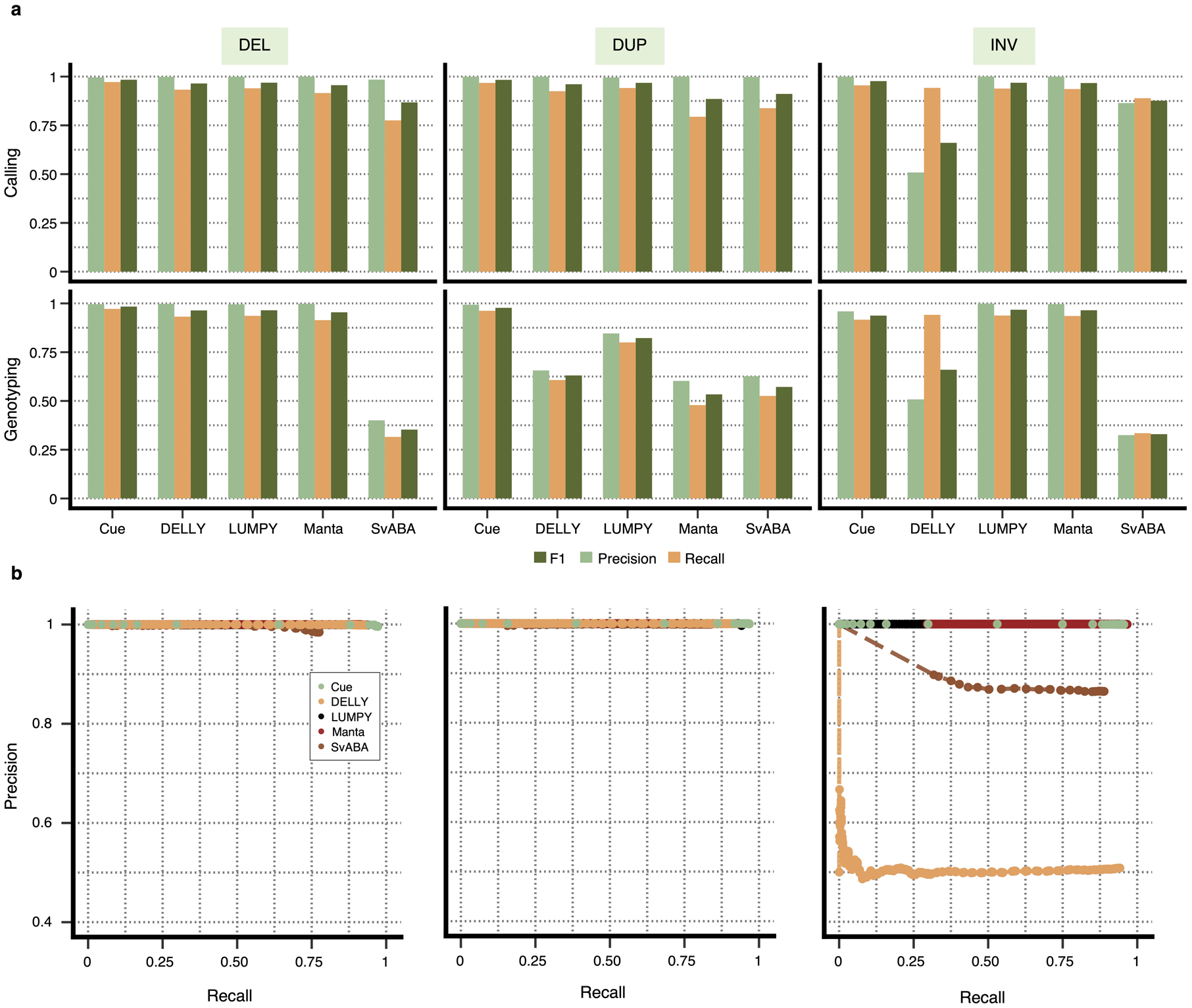
Performance evaluation broken down by SV type on synthetic data at 30x genome coverage. a. Precision, recall, and F1 score for DEL, DUP, and INV calling and genotyping. b. Recall-precision curves for each SV type generated using the SV quality thresholds reported in the QUAL VCF field.

Extended Data Fig. 2.

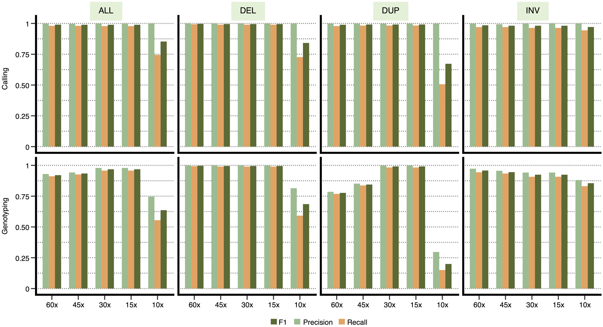
Performance evaluation on synthetic data at varying genome coverage. Precision, recall, and F1 score for DEL, DUP, and INV calling and genotyping computed for chr1 at 10x, 15x, 30x, 45x, and 60x genome coverage. Results are shown for all the SV calls combined (‘ALL’) and broken down by type.

Extended Data Fig. 3.

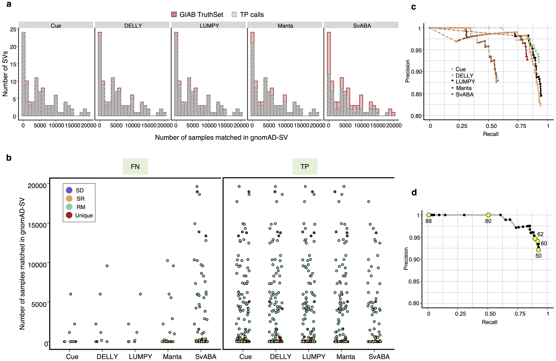
Evaluation of the TP, FN, and FP SV calls in the HG002 benchmark. a. Histogram showing the number of occurrences of the TP and FN SV calls in gnomAD-SV for each tool. SVs with no match in gnomAD-SV are collected in the zeroth bin. b. TP and FN calls broken down by frequency in gnomAD-SV and genome context. c. Recall-Precision curves generated using the SV quality thresholds reported in the QUAL VCF field. d. The Recall-Precision curve of Cue annotated with a subset of reported SV quality values.

Extended Data Fig. 4.

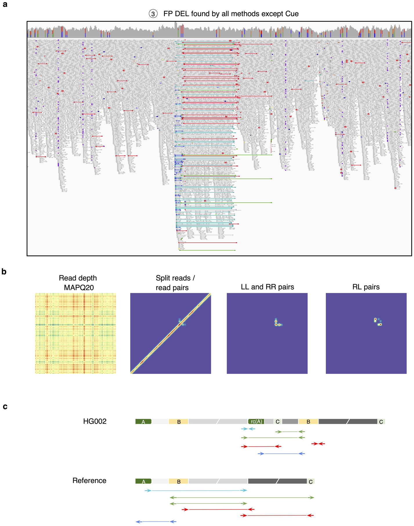
Analysis of a false positive HG002 deletion generated by all short-read callers except Cue. a. IGV plot showing short-read alignments at the call locus. Discordant read pairs mapped to the same strand (LL and RR mappings) are shown in light and dark blue, RL mappings are shown in green, and read pairs with a discordantly large insert size are shown in red. b. Cue-generated image channels depicting short-read signals that are inconsistent with a valid DEL signature. c. One of the two haplotypes of HG002, reconstructed by de novo assembly of PacBio CCS reads, that explains the main discordant pair mappings in panel a (the other haplotype is identical to the reference). The reconstructed haplotype contains two dispersed DUPs, one inverted dispersed DUP, and no DEL. Colored blocks labeled with letters are distinct short repeats. Gray blocks broken by diagonal lines are long sequences. rc(A) denotes the reverse-complement of A. Haplotypes were reconstructed and compared to the reference as follows. Let W be the sequence of the reference that covers the main patterns of discordant pairs in panel a. We built a joint de Bruijn graph (k=87) on W and on the 190 CCS reads that have some alignment to W, we removed k-mers with frequency one, and we translated W and every read into a walk (which may contain cycles) in the graph.

Extended Data Fig. 5.

Schematic of read-pair mapping signatures for a small dispersed DUP and a divergent reference repeat. Locus ‘A’ is duplicated in the donor genome. Some read pairs map discordantly in the RL orientation (green) or with a large insert size (red). Pairs internal to each copy of the donor map to the single copy of ‘A’ in the reference genome, doubling its coverage. If the reference has a divergent copy of ‘A’ (denoted as ‘a’), a gap in coverage will be observed at ‘a’.

Extended Data Fig. 6.

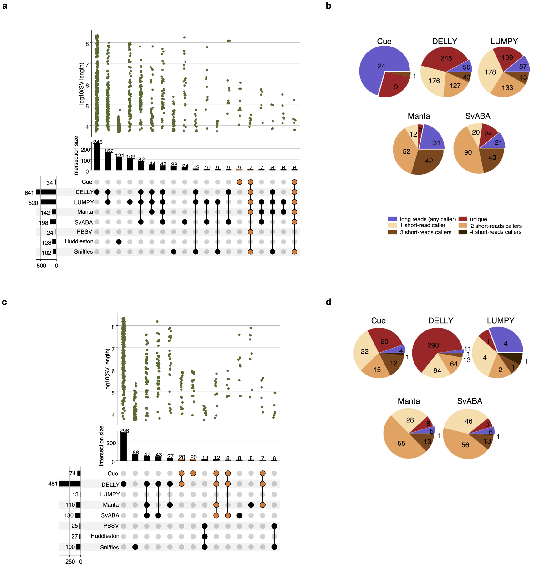
Evaluation of DUP and INV calls in the CHM1+CHM13 benchmark. a. Upset plot depicting DUP callset overlaps of short-read and long-read callers (only sets larger than 5 events are displayed for conciseness). Overlaps that include Cue are highlighted in orange. b. Breakdown of DUP calls by consensus with long-read and other short-read callers. c. Upset plot depicting INV callset overlaps of short-read and long-read callers. d. Breakdown of INV calls by consensus with long-read and other short-read callers.

Extended Data Fig. 7.

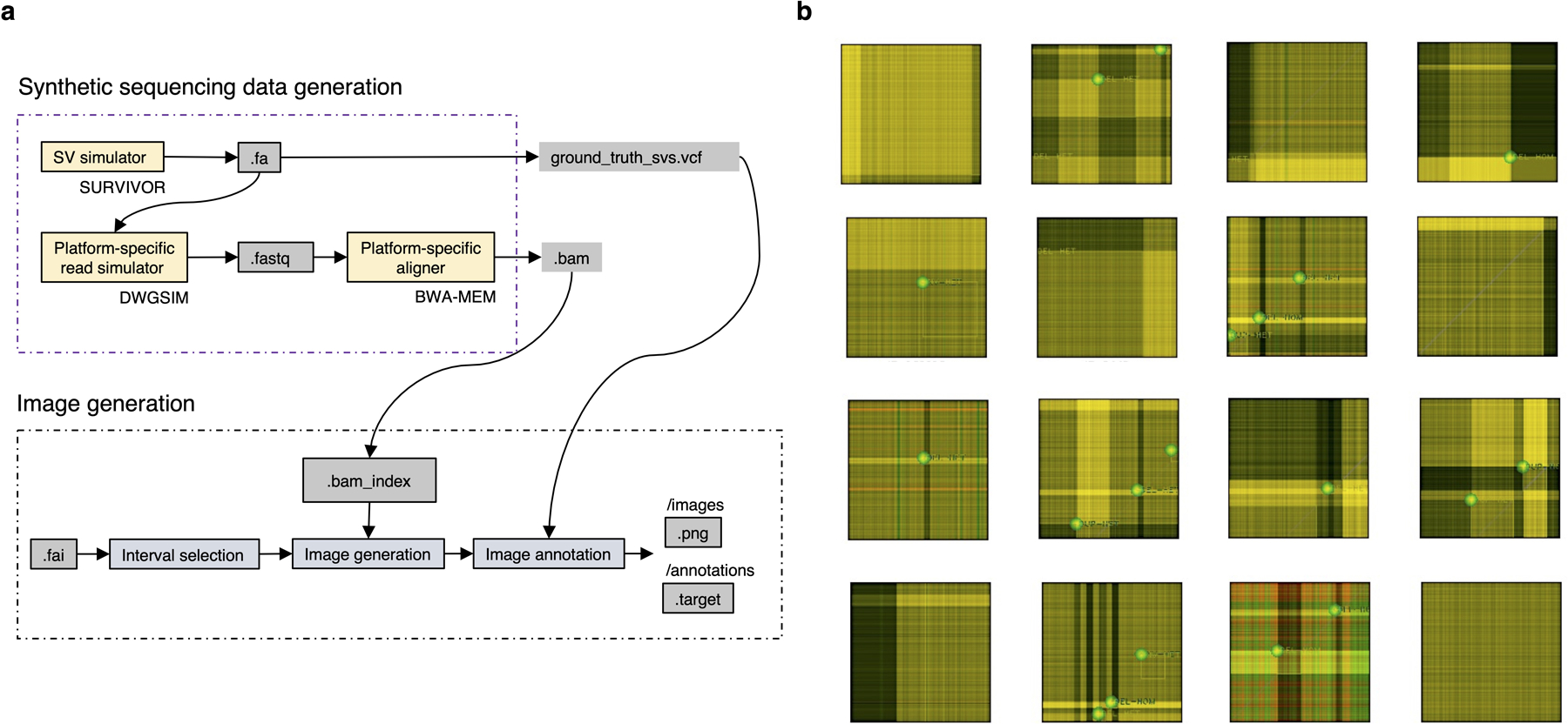
Training data generation. a. High-level overview of the in-silico sequencing and image data generation process. b. Annotated training examples (displayed using standard image visualization software using only three Cue channels, including the read-depth channel).

Extended Data Fig. 8.

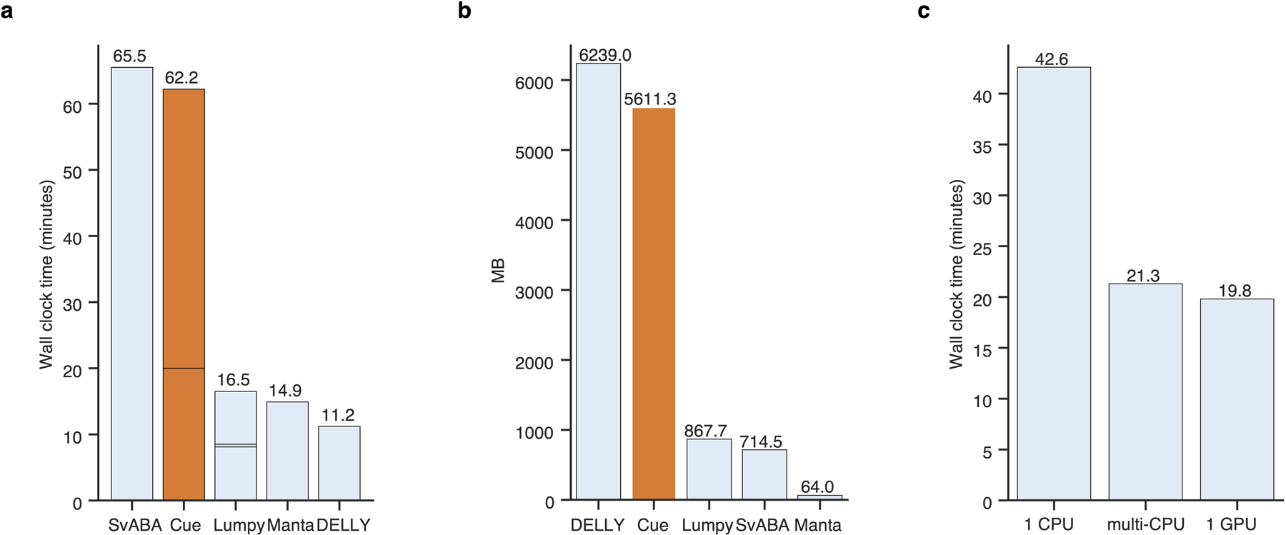
Runtime and memory performance on chr1 of HG002. a. Sequential runtime. Cue’s runtime is divided into indexing and calling. Lumpy’s runtime is divided into indexing, calling (short block), and genotyping. b. Sequential peak memory. c. Effect of PyTorch parallelism on calling time of Cue. In ‘multi-CPU’ mode we do not limit PyTorch to use a specific number of threads.

Data availability

The 60x HG002 Illumina WGS short reads, the 28x HG002 PacBio CCS reads, and the HG002 v0.06 truthset are available through the GIAB FTP data repository. In particular, short reads can be downloaded from https://ftp-trace.ncbi.nlm.nih.gov/giab/ftp/data/AshkenazimTrio/HG002_NA24385_son/NIST_HiSeq_HG002_Homogeneity-10953946/NHGRI_Illumina300X_AJtrio_novoalign_bams/HG002.hs37d5.60x.1.bam, the PacBio CCS reads can be downloaded from https://ftp-trace.ncbi.nlm.nih.gov/giab/ftp/data/AshkenazimTrio/HG002_NA24385_son/PacBio_CCS_15kb/alignment/HG002.Sequel.15kb.pbmm2.hs37d5.whatshap.haplotag.RTG.10x.trio.bam, and the v0.06 truthset can be downloaded from https://ftp-trace.ncbi.nlm.nih.gov/giab/ftp/data/AshkenazimTrio/analysis/NIST_SVs_Integration_v0.6/HG002_SVs_Tier1_v0.6.vcf.gz. The CHM1 and CHM13 40x coverage Illumina WGS short reads can be downloaded from the ENA short read archive (ENA accessions ERR1341794 and ERR1341795, respectively). The CHM1 and CHM13 PacBio long reads can be obtained from the NCBI sequence read archive under accession numbers SRP044331 (CHM1) and SRR11292120-SRR11292123 (CHM13). The Huddleston et al. [41] CHM1 and CHM13 truthsets can be downloaded from http://eichlerlab.gs.washington.edu/publications/Huddleston2016/structural_variants. To obtain a single truthset, we merged the CHM1 and CHM13 VCFs using SURVIVOR and genotyped the calls accordingly (i.e. such that records reported in both CHM1 and CHM13 were labeled as homozygous, and records only reported in one of the two were labeled as heterozygous). To label duplications, we cross-referenced insertion calls with Supplementary Table 11 of [41], which separately reports which published insertion calls are duplications. The synthetic benchmark data, training data, trained models, and configurations are available through the associated GitHub repository: https://github.com/PopicLab/cue.

References

- [1].Chaisson Mark JP et al. “Multi-platform discovery of haplotype-resolved structural variation in human genomes”. In: Nature Communications 10.1 (2019), pp. 1–16. [DOI] [PMC free article] [PubMed] [Google Scholar]
- [2].Mantere Tuomo, Kersten Simone, and Hoischen Alexander. “Long-read sequencing emerging in medical genetics”. In: Frontiers in Genetics 10 (2019), p. 426. [DOI] [PMC free article] [PubMed] [Google Scholar]
- [3].Li Yilong et al. “Patterns of somatic structural variation in human cancer genomes”. In: Nature 578.7793 (2020), pp. 112–121. [DOI] [PMC free article] [PubMed] [Google Scholar]
- [4].Chen Xiaoyu et al. “Manta: rapid detection of structural variants and indels for germline and cancer sequencing applications”. In: Bioinformatics 32.8 (2016), pp. 1220–1222. [DOI] [PubMed] [Google Scholar]
- [5].Rausch Tobias et al. “DELLY: structural variant discovery by integrated paired-end and split-read analysis”. In: Bioinformatics 28.18 (2012), pp. i333–i339. [DOI] [PMC free article] [PubMed] [Google Scholar]
- [6].Layer Ryan M. et al. “LUMPY: a probabilistic framework for structural variant discovery.” eng. In: Genome Biology 15.6 (2014), R84. [DOI] [PMC free article] [PubMed] [Google Scholar]
- [7].Wala Jeremiah A et al. “SvABA: genome-wide detection of structural variants and indels by local assembly.” In: Genome Research (Mar. 2018). [DOI] [PMC free article] [PubMed] [Google Scholar]
- [8].Sedlazeck Fritz J et al. “Accurate detection of complex structural variations using single-molecule sequencing”. In: Nature Methods 15.6 (2018), pp. 461–468. [DOI] [PMC free article] [PubMed] [Google Scholar]
- [9].Pacific Biosciences. pbsv. https://github.com/PacificBiosciences/pbsv. 2018. [Google Scholar]
- [10].Alkan Can, Coe Bradley P, and Eichler Evan E. “Genome structural variation discovery and genotyping”. In: Nature Reviews Genetics 12.5 (2011), pp. 363–376. [DOI] [PMC free article] [PubMed] [Google Scholar]
- [11].Poplin Ryan et al. “A universal SNP and small-indel variant caller using deep neural networks”. In: Nature Biotechnology 36.10 (2018), pp. 983–987. [DOI] [PubMed] [Google Scholar]
- [12].Belyeu Jonathan R et al. “Samplot: a platform for structural variant visual validation and automated filtering”. In: Genome Biology 22.1 (2021), pp. 1–13. [DOI] [PMC free article] [PubMed] [Google Scholar]
- [13].Bai Ruofei et al. “Cnngeno: A high-precision deep learning based strategy for the calling of structural variation genotype”. In: Computational Biology and Chemistry 94 (2021), p. 107417. [DOI] [PubMed] [Google Scholar]
- [14].Liu Yongzhuang et al. “A deep learning approach for filtering structural variants in short read sequencing data”. In: Briefings in bioinformatics 22.4 (2021), bbaa370. [DOI] [PubMed] [Google Scholar]
- [15].Cai Lei, Wu Yufeng, and Gao Jingyang. “DeepSV: accurate calling of genomic deletions from high-throughput sequencing data using deep convolutional neural network”. In: BMC Bioinformatics 20.1 (2019), pp. 1–17. [DOI] [PMC free article] [PubMed] [Google Scholar]
- [16].Newell Alejandro, Yang Kaiyu, and Deng Jia. “Stacked hourglass networks for human pose estimation”. In: European Conference on Computer Vision. Springer. 2016, pp. 483–499. [Google Scholar]
- [17].Newell Alejandro, Huang Zhiao, and Deng Jia. “Associative embedding: End-to-end learning for joint detection and grouping”. In: arXiv preprint arXiv:1611.05424 (2016). [Google Scholar]
- [18].Zook Justin M et al. “A robust benchmark for detection of germline large deletions and insertions”. In: Nature Biotechnology 38.11 (2020), pp. 1347–1355. [DOI] [PMC free article] [PubMed] [Google Scholar]
- [19].Li Heng et al. “A synthetic-diploid benchmark for accurate variant-calling evaluation”. In: Nature Methods 15.8 (2018), pp. 595–597. [DOI] [PMC free article] [PubMed] [Google Scholar]
- [20].Huddleston John et al. “Discovery and genotyping of structural variation from long-read haploid genome sequence data”. In: Genome Research 27.5 (2017), pp. 677–685. [DOI] [PMC free article] [PubMed] [Google Scholar]
- [21].Li Jia, Su Wen, and Wang Zengfu. “Simple pose: Rethinking and improving a bottom-up approach for multi-person pose estimation”. In: Proceedings of the AAAI Conference on Artificial Intelligence. Vol. 34. 07. 2020, pp. 11354–11361. [Google Scholar]
- [22].Jeffares Daniel C et al. “Transient structural variations have strong effects on quantitative traits and reproductive isolation in fission yeast”. In: Nature Communications 8.1 (2017), pp. 1–11. [DOI] [PMC free article] [PubMed] [Google Scholar]
- [23].English Adam C et al. “Truvari: Refined structural variant comparison preserves allelic diversity”. In: bioRxiv (2022). [DOI] [PMC free article] [PubMed] [Google Scholar]
- [24].Tarailo-Graovac Maja and Chen Nansheng. “Using RepeatMasker to identify repetitive elements in genomic sequences”. In: Current Protocols in Bioinformatics 25.1 (2009), pp. 4–10. [DOI] [PubMed] [Google Scholar]
- [25].Karolchik Donna et al. “The UCSC Genome Browser database”. In: Nucleic Acids Research 31.1 (2003), pp. 51–54. [DOI] [PMC free article] [PubMed] [Google Scholar]
- [26].Zhao Xuefang et al. “Expectations and blind spots for structural variation detection from long-read assemblies and short-read genome sequencing technologies”. In: The American Journal of Human Genetics (2021). [DOI] [PMC free article] [PubMed] [Google Scholar]
- [27].Collins Ryan L et al. “A structural variation reference for medical and population genetics”. In: Nature 581.7809 (2020), pp. 444–451. [DOI] [PMC free article] [PubMed] [Google Scholar]
- [28].Ono Yukiteru, Asai Kiyoshi, and Hamada Michiaki. “PBSIM2: a simulator for long-read sequencers with a novel generative model of quality scores”. In: Bioinformatics 37.5 (2021), pp. 589–595. [DOI] [PMC free article] [PubMed] [Google Scholar]
- [29].Li Heng. “Minimap2: pairwise alignment for nucleotide sequences”. In: Bioinformatics 34.18 (2018), pp. 3094–3100. [DOI] [PMC free article] [PubMed] [Google Scholar]
- [30].Luo Ruibang et al. “LRSim: a linked-reads simulator generating insights for better genome partitioning”. In: Computational and Structural Biotechnology Journal 15 (2017), pp. 478–484. [DOI] [PMC free article] [PubMed] [Google Scholar]
- [31].Marks Patrick et al. “Resolving the full spectrum of human genome variation using Linked-Reads”. In: Genome Research 29.4 (Mar. 2019), pp. 635–645. [DOI] [PMC free article] [PubMed] [Google Scholar]
- [32].Fang Li et al. “LinkedSV for detection of mosaic structural variants from linked-read exome and genome sequencing data”. In: Nature Communications 10.1 (2019), pp. 1–15. [DOI] [PMC free article] [PubMed] [Google Scholar]
- [33].Ebert Peter et al. “Haplotype-resolved diverse human genomes and integrated analysis of structural variation”. In: Science 372.6537 (2021). [DOI] [PMC free article] [PubMed] [Google Scholar]
- [34].Thorvaldsdóttir Helga, Robinson James T, and Mesirov Jill P. “Integrative Genomics Viewer (IGV): high-performance genomics data visualization and exploration”. In: Briefings in Bioinformatics 14.2 (2013), pp. 178–192. [DOI] [PMC free article] [PubMed] [Google Scholar]
- [35].DWGSIM. https://github.com/nh13/DWGSIM.
- [36].Li Heng. “Aligning sequence reads, clone sequences and assembly contigs with BWA-MEM”. In: arXiv preprint arXiv:1303.3997 (2013). [Google Scholar]
- [37].Newell Alejandro, Yang Kaiyu, and Deng Jia. “Stacked hourglass networks for human pose estimation”. In: European Conference on Computer Vision. Springer. 2016, pp. 483–499. [Google Scholar]
- [38].Newell Alejandro, Huang Zhiao, and Deng Jia. “Associative embedding: End-to-end learning for joint detection and grouping”. In: arXiv preprint arXiv:1611.05424 (2016). [Google Scholar]
- [39].Kingma Diederik P and Ba Jimmy. “Adam: A method for stochastic optimization”. In: arXiv preprint arXiv:1412.6980 (2014). [Google Scholar]
- [40].Li Jia, Su Wen, and Wang Zengfu. “Simple pose: Rethinking and improving a bottom-up approach for multi-person pose estimation”. In: Proceedings of the AAAI Conference on Artificial Intelligence. Vol. 34.07. 2020, pp. 11354–11361. [Google Scholar]
- [41].Huddleston John et al. “Discovery and genotyping of structural variation from long-read haploid genome sequence data”. In: Genome Research 27.5 (2017), pp. 677–685. [DOI] [PMC free article] [PubMed] [Google Scholar]
- [42].Popic Victoria et al. Cue (Version 2.0). 10.24433/CO.8949236.v2. Code Ocean, 2022. [DOI] [Google Scholar]
Associated Data
This section collects any data citations, data availability statements, or supplementary materials included in this article.
Supplementary Materials
Data Availability Statement