

Abstract
Deep neural networks (DNNs) have advanced our ability to take DNA primary sequence as input and predict a myriad of molecular activities measured via high-throughput functional genomic assays. Post hoc attribution analysis has been employed to provide insights into the importance of features learned by DNNs, often revealing patterns such as sequence motifs. However, attribution maps typically harbor spurious importance scores to an extent that varies from model to model, even for DNNs whose predictions generalize well. Thus, the standard approach for model selection, which relies on performance of a held-out validation set, does not guarantee that a high-performing DNN will provide reliable explanations. Here we introduce two approaches that quantify the consistency of important features across a population of attribution maps; consistency reflects a qualitative property of human interpretable attribution maps. We employ the consistency metrics as part of a multivariate model selection framework to identify models that yield high generalization performance and interpretable attribution analysis. We demonstrate the efficacy of this approach across various DNNs quantitatively with synthetic data and qualitatively with chromatin accessibility data.
1. Introduction
Deep neural networks (DNNs) have demonstrated a powerful ability to learn complex sequence-function relationships from high-throughput functional genomics data, taking DNA sequences as input and predicting functional activities, such as transcription factor binding and chromatin accessibility [1, 2, 3, 4, 5]. The improved predictions by DNNs suggest that they are learning biological knowledge not considered by existing, traditional models, such as position weight matrices or -mers. Distilling the rationale underlying their improved predictions through model interpretability is key to realizing the transformative impact that DNNs can bring to genomics.
Many regulatory functions are controlled though protein-DNA interactions. Proteins bind to DNA with varying degrees of affinity, depending on expression levels and sequence context [6]. Strong binding sites are typically summarized as sequence motifs. One major goal of model interpretability is to reveal motifs and their dependencies that drive model predictions.
Of the many approaches to explainable AI [7, 8], attribution methods comprise a set of techniques that provide a base-resolution map of importance scores for each nucleotide in a given input sequence on model predictions [9, 10, 11, 12, 13, 14]. Attribution scores have a natural interpretation as single-nucleotide variant effects [15]. Attribution maps have demonstrated an ability to reveal known motifs that are important for cell-type specific regulatory functions and annotate their positions at base resolution [16, 17, 18]. Since attribution methods provide local explanations [19], i.e. for one datapoint, it is imperative to observe several attribution maps to deduce generalizable patterns.
The high expressivity of DNNs gives them the power to learn complex sequence-function relationships, but it also makes it easier to achieve benign overfitting [20, 21], which is an empirical phenomenon where the training and test performance diverge throughout training. While this is classically recognized in machine learning as overfitting, it turns out for highly flexible models, such as DNNs, benign overfitting does not necessarily affect generalization performance even though a more complex function is being learned to “overfit” the training data [22]. Nevertheless, it can adversely affect the quality of attribution maps which depends on the local properties of the function [23, 24], making it difficult to disentangle functional motifs from nucleotides with spurious importance scores. This suggests that DNNs can yield reliable or unreliable attribution maps and the generalization performance is largely not informative to identify which DNNs are more amenable with attribution analysis. This problem is exacerbated by the lack of ground truth with real biological data, which makes it difficult to quantitatively assess the efficacy of attribution maps.
Here we propose two quantitative metrics that characterize the consistency of position-invariant local patterns that are shared across a population of attribution maps. Importantly, this approach does not require any ground truth knowledge as it aims to characterize qualitative properties of attribution maps that are human interpretable. We present results that show our consistency metrics are highly correlated to the quality of attribution maps both quantitatively across various models trained on synthetic data and qualitatively on in vivo genomics data. This work provides a foundation for a multivariate model selection framework to identify DNNs that yield high generalization and robust interpretations in real world genomic applications.
2. Characterizing consistency of attribution maps
In many regulatory genomic prediction tasks, we expect that important patterns such as motifs are stationary features and thus should appear more consistently while spurious noise should not be shared across genomic loci. Thus a measure of the consistency of motif patterns (and the level of spurious importance scores) across attribution maps captures a qualitative property that should provide insights into the reliability of attribution maps. Below, we introduce two information-based summary statistics that aim to quantify the level of consistency in local patterns shared across a population of attribution maps. These methods are based on: 1) the distribution of -mers within attributed positions and 2) the distribution of attribution scores in a low-dimensional contextual embedding space.
2.1. -mer Method: KL-divergence of attributed -mers versus an uninformative prior
The motivation for this method is based on the observation that patterns in reliable attribution maps should enrich for motifs, which can be represented with a specific distribution of -mers. This distribution should be more sparse compared to a baseline -mer distribution across all positions in the sequences. On the other hand, we expect poor quality attribution maps to have a more diffuse distribution that closely resembles the baseline -mer distribution. Thus, the distance between the -mer distributions within attributed positions or across all positions may provide a sensitive metric to compare attribution map consistency (Fig. 1).
Figure 1:

Schematic of consistency metrics. (a) -mer Method: KLD of attributed -mer frequencies versus an uninformative prior. (b) -attr-mean Method: KLD of the distribution of locally averaged attribution vectors versus an uninformative prior.
To measure the distance between the -mer distributions, we utilize the Kullback-Leibler divergence (KLD) (Fig. 1a). To calculate the KLD, we need to: 1) choose a -mer size; 2) define which positions are within significant attribution scores; and 3) calculate global -mer frequencies across all positions. To identify attributed positions, we applied a sequence-specific threshold to each attribution map in the test set, above which are considered attributed positions. This type of threshold aims to address the variable magnitudes in the attribution maps from sequence to sequence. The threshold was set automatically for each sequence according to the 90th percentile in the attribution scores. For each set of contiguous positions, we added a buffer size of 2 nucleotides on the 3’ end to extend the positions considered. While this step introduces some noise, it also helps to address motif positions that have variable attribution scores (some below and some above the threshold), which is a prevalent feature of noisy attribution maps. Global -mer frequencies were then calculated by aggregating the -mer frequencies within each of the subsequences which had a minimum length of . In this study, . For comparison, a non-informative empirical prior was calculated by aggregating the -mer frequencies across all test sequences. We then calculated the KLD between the two -mer frequencies in an element-wise fashion and summed them to get a single summary statistic.
2.2. -attr-mean Method: KL-divergence of the distribution of locally embedded attribution scores versus an uninformative prior
To encode information about the local structure of motifs, we construct a new metric that considers a lower-dimensional embedding based on locally averaged attribution maps. Specifically, we first apply a gradient correction which effectively fixes the gauge freedom in attribution maps which arises due to the nature of one-hot encoded DNA [25]. Given a corrected attribution map, , we calculate the mean attribution scores (across each nucleotide channel) with a window size of centered on each position. This provides local context of nearby attribution scores similar to a uniform convolutional kernel. In this paper, . Each 4-dimensional (4D) mean attribution vector is reduced to 3D with a Gram-Schmidt orthogonalization procedure to remove the linear dependence (see Appendix A), which arises from gauge fixing with the gradient correction. This enables a direct visualization of (averaged) attribution vectors in 3D space. Strikingly, the mean attribution vectors exhibit a high degree of structure with radial symmetry (Fig. 1b). Since the natural coordinates are spherical, we further reduce the dimensions into 2D space by considering the 2 angular components (i.e. polar and azimuthal), while using the inverse squared radius as a weight for this 2D distribution. As in Method 1, we apply a filter based on a threshold set by the 90th percentile of the attribution scores for each sequence. We then bin the filtered points within the 2D angular space with a uniform lattice of size 0.1 radians, adding the weights (i.e. squared radius) within each bin. This is followed by a global normalization to make the sum of all bins equal to 1. This serves as a coarse-grain angular density of attributed positional vectors.
To construct a non-informative prior, we apply a boxcar filter (with a window size 0.5 radians) to diffuse the cluster information while retaining global spatial biases. We note that the observed bias within the uninformative prior arises from the asymmetry in attribution scores; important motifs typically yield positive attribution scores. In addition, spatial distortions due to projecting a 3D globe onto a 2D map contributes to spatial biases. The KLD between the two distributions is then calculated separately within each bin and summed to provide a single summary statistic. Henceforth, we refer to method 2 as -attr-mean.
3. Comparing models for binary classification of synthetic regulatory codes
To test how well the proposed consistency metrics can facilitate a model selection scheme that is amenable to biological discovery from attribution analysis, we explored several hundred DNNs trained with different regularization strategies on a synthetic regulatory genomic prediction task from Ref. [26]. This dataset is ideal as it uses synthetic data, for which we have “pixel-level” ground truth, and it compares a diverse set of models, of which many regularization strategies have support for improving attribution maps. This allows us to test the efficacy of the consistency metrics across various DNNs (with similar generalization performance) with a direct comparison to a summary statistic that captures the reliability of their attribution maps.
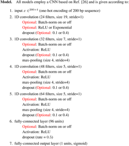
Briefly, the task consists of taking 200 nucleotide DNA sequences as input and predicting a binary classification of whether the sequence contains at least 3 “core motifs” (up to 5) in any combinations (positive class) or contains a different set of “background motifs” (negative class). This synthetic data consists of 20,000 total sequences split randomly into a training (0.7), validation (0.1), and test (0.2) set. The baseline DNN that was used here consists of 4 convolutional layers and 1 fully connected layer with optional batch normalization prior to each activation and the first layer activation being either ReLU or exponential, which was shown to lead to more interpretable attribution maps. Using these base architectures, 327 model variations were explored with different regularization strategies – input mixup [27], manifold mixup [28], input noise [29], manifold noise, adversarial training and spectral norm regularization [30]. Further details regarding the specific models used are given in Appendix B.
We trained each model with different random initializations for a total of 390 DNNs. Of these, 327 DNNs passed a performance filter with an area-under the receiver operating characteristic curve (AUROC) cutoff of 0.97. For each high performing DNN, we calculated an attribution map for all positive label sequences. We then calculated the signal-to-noise ratio (SNR) by defining signal as the average attribution scores at positions where ground truth motifs are embedded, while background was calculated according to the average of the top 10 highest false-positive attribution scores. The ratio provides a measure of the signal strength compared to the worst false positive attributions in background positions, which better reflects the practical scenario where motif discoveries are based on positive attribution scores.
As expected, we observed that the generalization performance on the test set does not correlate with the attribution SNR of each DNN’s attribution maps (Fig. 2a and Fig. 4 in Appendix C), in agreement with previous observations [26, 25]. Many DNNs yield high predictions but their attribution SNR can vary significantly. Thus, when scientific discovery based on attribution analysis is a major downstream application, as is frequently used in genomics, there must be an additional metric that can further stratify these models to sub-select DNNs that yield both high generalization performance and more human-interpretable attribution analysis.
Figure 2:
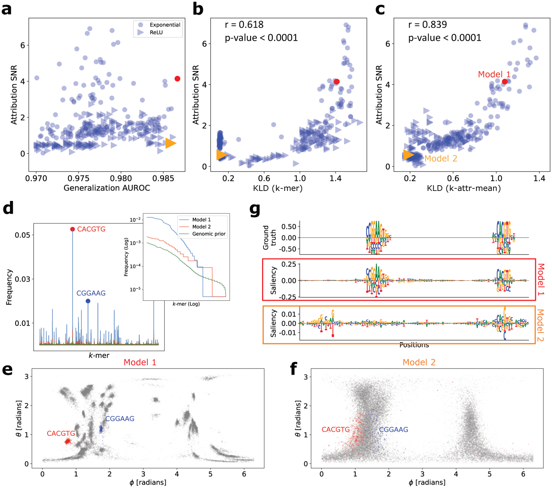
Performance of consistency metrics on synthetic data. (a) Scatter plot of generalization AUROC and attribution SNR (based on saliency maps) for various DNNs trained with different regularization methods on synthetic data. Each point represents a different model and the marker represents whether the first layer activation was ReLU or exponential. (b,c) Scatter plot of attribution SNR versus the consistency metric defined by KLD of -mer (b) and -attr-mean (c). (d) -mer frequency distribution for Model 1, Model 2, and an empirical prior (shown in a different color). Inset shows the ranked list of the same -mer distribution as a log-log plot. (e,f) Density of the angular components of lower-dimensional embedding for Model 1 (left) and Model 2 (right). (g) Saliency map comparison for a representative test set sequence for Model 1 and Model 2. Ground truth is shown at the top for reference. Sequence logos were generated using Logomaker [31].
The strategy that we propose is based on consistency metrics (Sec. 2.1 and 2.2). However, in order to be useful for model selection, the consistency metric must be able to track the attribution SNR of attribution analysis, because in real world settings, ground truth in attribution maps is not known. To test this, we plot the attribution SNR versus each consistency metric (Fig. 2b for -mer method and Fig. 2c for -attr-mean method). While not a perfect one-to-one correlation, the consistency metrics capture general trends that should inform which model’s attribution maps are more interpretable even when ground truth in attribution maps do not exist (see Table 1 in Appendix C for full results).
Upon further investigation, we consider 2 DNNs that yield similar high generalization performance but very different attribution SNRs, i.e. Model 1 exhibits a higher attribution SNR compared to Model 2. For the -mer consistency method, models that learn more consistent motifs exhibit more skew in the -mer distribution (Fig. 2d), with a subset of -mers exhibiting higher frequencies within attributed positions compared to a non-informative prior, as expected. For the -attr-mean consistency method, we observe a trend where mean attribution vectors are clustered in the 2D-embedded angle space, with tighter clusters corresponding to DNNs with higher attribution SNR (Fig. 2e and 2f). Surprisingly, we found that the sequences that correspond to a given cluster are often the same and represent (parts of) known motifs. Interestingly, we find that each consistency-based method identifies similar motifs for Model 1 (Fig. 2d and 2e), while Model 2 remains much more difficult to decipher. Moreover, a qualitative comparison of saliency maps shows that Model 1 indeed visually reflects ground truth patterns relative to Model 2 (Fig. 2g). While the main results are presented for saliency maps, similar conclusions would be drawn using other attribution maps, including integrated gradients and smoothgrad (Fig. 5 in Appendix C).
An investigation into the sensitivity of each methods hyperparameters (i.e. and attribution threshold for -mer and -attr-mean methods) shows that the same conclusions would largely be drawn from different hyperparameter choices (Fig. 6 in Appendix C). Nevertheless, the sensitivity, which is the separation of the KLD between different models, is sensitive to hyperparameters; optimal values can be selected based on observing a larger spread of KLD across models on the validation set.
4. Comparing models that predict chromatin accessibility profiles
To assess the generalization of the two proposed consistency metrics, we compared how well each method facilitates model selection based on the attribution maps across 26 previously trained DNNs from Ref. [33]. In this study, the task is to take 2048 nt one-hot DNA sequences as input and predict 15 chromatin accessibility profiles experimentally measured by ATAC-seq (Assay for Transposase-Accessible Chromatin using sequencing) in human cell lines. Specifically, DNNs were trained either as a binary classification of statistically significant peaks identified in the read coverage profiles or a quantitative regression that directly predicts the read coverage profiles at various resolutions. This study provides an ideal platform to explore our model selection scheme as it is comprised of numerous models trained with various architectures and data augmentations. Further details regarding the specific models used in this study is given in in Ref. [33] and Table 2 in Appendix C.
Without loss of generality, we focused our study on 3,968 saliency maps from sequences that corresponds to high read coverage for the GM12878 cell line (1 of the 15 cell lines). By considering both the generalization performance and consistency metric for model selection, we found that the highest performing DNNs did not yield the most consistent attribution maps (Figs. 3a and 3b). Interestingly, we identified a three models from each stratified group that generalized nearly as well on the test set but whose consistency metric scaled differently. We note that the -attr-mean method exhibited a wider separation compared to the -mer method, suggesting that it has a higher sensitivity (see Table 2 in Appendix C for full results). By qualitatively comparing the sequence logos of the attribution maps from each of these models, we observed that the KLD value agrees with our expectations; the model with higher KLD visually captures known motifs better than the other models that have lower KLDs (Figs. 3F and 3d).
Figure 3:
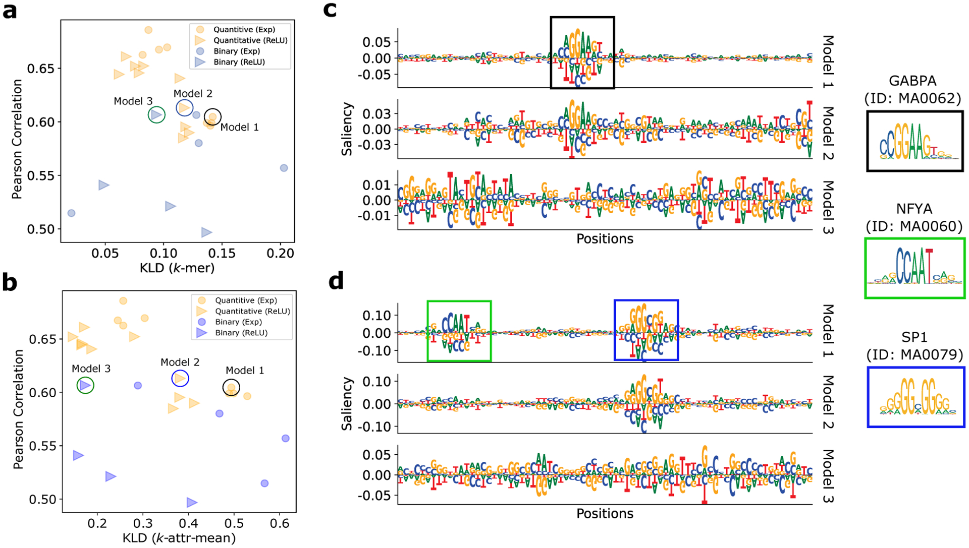
Selecting interpretable DNNs trained on chromatin accessibility data. Scatter plot of Pearson correlation of the test performance versus the consistency metric (KLD) calculated from the -mer method (a) and the -attr-mean method (b) for various DNNs trained on ATAC-seq data for GM12878. Each dot represents a different model with a color and marker combination that stratifies with modeling choice, i.e. quantitative models and binary models and their first layer activation function, ReLU or exponential. (c,d) Saliency maps for three different models from two representative test sequence. Sequence logos were generated using Logomaker [31]. Annotated motifs from the JASPAR database [32] are shown on the right.
5. Discussion
Interpreting high-performing DNNs through attribution analysis can provide new biological insights about motifs and their syntax. However, the current strategy to select which model to interpret is based on held out validation performance, which does not necessarily guarantee the model’s attribution maps will be visually human-interpretable. Hence there must be an additional metric as part of a multivariate model selection process to identify optimal models with good generalization and reliable attribution methods. Here we propose 2 metrics that characterize the consistency of important features in attribution maps. One approach is based on a simple -mer distribution within attributed positions and the second is based on the distribution of local attribution embeddings. We find that both approaches work well in practice, though the limits of each method have not been explored thoroughly in this study. We find that the -mer consistency metric is valuable as a simple and quick estimate that can eliminate most models with low attribution SNR and narrow down the search for models with high attribution SNR, while the -attr-mean consistency metric shows more sensitivity to track attribution SNR. Together, this demonstrates that it may be beneficial to incorporate consistency-based KLD as a secondary metric in addition to generalization performance.
Motif discovery and annotation.
Interestingly, the intermediate processing steps in both consistency metrics show promise for de novo motif discovery (Fig. 2d and 2e). These aggregated statistics can help to uncover global motifs that are consistently learned across attribution maps, providing a complementary approach to an existing clustering tool TF-MoDISCo [34]. Further development could exploit these intermediate representations to annotate motifs in individual sequences.
Limitations of attribution analysis.
Although the goal here is to help identifiability of optimal models that would yield more interpretable attribution maps, attribution maps are anecdotal views of single nucleotide effects in a given sequence. It does not specify the effect size of extended patterns, such as motifs or combinations of motifs. Nevertheless, more reliable attribution maps facilitates hypotheses generation of cis-regulatory mechanisms that can be followed up with in silico experiments, such as global importance analysis [35].
Limitations of this study.
The proposed consistency metrics were motivated by the desire to characterize consistent motifs in attribution maps. However, the importance of motifs may be influenced by the presence of another motif or sequence context. These can make attribution scores for motifs more diffuse for reasons that appear as a less consistent attribution maps. Another limitation is that as the number of tasks grow, consistency-based metrics can suffer from an over-crowded set of important patterns, which may lead to reduced sensitivity. Moreover, models that learn a small subset of features well would yield higher KLD compared to a model that learns a broader set of patterns, which may be a more comprehensive characterization of regulatory DNA. Thus, an additional property that would be desirable is to capture the diversity of consistent patterns, thereby providing another axis that can be utilized in a multivariate approach to model selection. Together, this work lays the groundwork to identify optimal models that would yield more trustworthy attribution analysis for robust scientific discovery in genomics.
Acknowledgements
Research reported in this publication was supported in part by the National Human Genome Research Institute of the National Institutes of Health under Award Number R01HG012131, the Developmental Funds from the CSHL Cancer Center Support Grant 5P30CA045508, and the Simons Center for Quantitative Biology at Cold Spring Harbor Laboratory. This work was performed with assistance from the US National Institutes of Health Grant S10OD028632-01. We would also like to thank Justin Kinney and David McCandlish for helpful discussions.
A. Gram-Schmidt orthogonalization
Gradient-corrected attribution maps ([25]) in genomic one-hot sequence data have scores that sum to zero at each position. This introduces linear dependency between the 4 scores at each nucleotide position. Linear dependency means that there is excess dimensionality in the data, so we may reduce it. We use the Gram-Schmidt (G-S) procedure to calculate new linear combinations that are linearly independent and orthogonal. For every nucleotide position, the 4-vector of scores we transform using
where and where .
This reduces the number of dimensions of the data from 4D to 3D, which is favorable from the calculation time perspective for later analysis. We do not lose any information by this change of basis.
B. Synthetic data analysis
Data.
The synthetic dataset consists of 20,000 sequences (each 200 nucleotides long) split randomly into a train, validation, and test set according to fractions 0.7, 0.1, and 0.2 , respectively. Each sequence is sampled from a single sequence model, , with elements equal to 0.25, except for where motifs were embedded. Positive sequences were embedded with 3 to 6 “core” motifs (i.e. CTCF, SP1, YY1, GABPA and SRF from the JASPAR database [32]), randomly drawn with replacement, while negative sequences were embedded with a bag of motifs that includes 50 additional background motifs. Since we know exactly where motifs are embedded during the simulation process, we have ground truth of the importance of various letters at different positions.
where is a factor to change the width of the network, here . By default, batch normalization [36] is applied prior to the activation of each hidden layer, and dropout [37] is incorporated after each convolutional layer with a default rate of 0.1 and the dense layer with 0.5.
We uniformly trained each model by minimizing the binary cross-entropy loss function with minibatch stochastic gradient descent (100 sequences) for 100 epochs with Adam [38] updates using default parameters. All reported performance metrics are drawn from the test set using the model parameters that yielded the highest performance metric on the validation set, i.e. early stopping.
Mixup.
Mixup is a data augmentation technique introduced by [27]. The key idea here is that the sensitivity of a DNN to adversarial examples may be reduced by imposing constraints that force the model to interpolate linearly between any two input points. Concretely, this is achieved by constructing augmented data samples as follows. Given a pair of datapoints, and from the training dataset, construct a new datapoint as a convex combination of the training sample pair:
| (1) |
where is sampled randomly from a beta distribution . The concentration parameter is a hyperparameter which is set to 1.
In practice, the augmented data samples are constructed by randomly permuting the order of the samples in a minibatch. Let denote a minibatch of size and denote the same minibatch with the ordering of it’s samples permuted randomly. The augmented minbatch is generated by applying Eqn. (1) to the original minibatch and its permuted form:
| (2) |
Manifold mixup.
Manifold mixup, proposed by [28], is a generalization of the mixup data augmentation scheme. Instead of ‘mixing up’ samples on the input manifold alone, as is the case with mixup, manifold mixup extends that principle to include mixing up the hidden representations (i.e. activations from the hidden layers) of the input as well. Consider a layer . Let be the input and for be the hidden representations of the input. Let be the set of indices of all NN layer activations before the final output and including the original input. Given , the NN can be expressed as . The manifold mixup augmentation scheme proceeds similarly to that of the mixup technique. Given a minibatch of data , we first sample and compute . The minibatch in this hidden representation is . We then randomly permute the order of the examples to obtain . Finally, we take a convex combination of our original and permuted minibatches to obtain the augmented minibatch:
| (3) |
where, and is a hyperparameter. In this work, is set to 1.
Input noise and manifold input noise.
Injecting noise into the input and hidden representation is a well-known regularizing technique [29]. Most notably, this takes the form of dropout [37] which applies a multiplicative mask sampled from a Bernoulli distribution. Theoretically, adding noise to the input data has been shown to be equivalent to adding an extra term to the loss function. More specifically, under a mean squared error loss function and zero-mean Gaussian noise injected into the input, it can be shown that this additional penalty is equivalent to a Tikhonov regularizer [39]. In our work, we explored 2 forms of regularizations based on noise injection.
For a input (with corresponding label ), we sample and add it to the input. This produces the perturbed input which leads to a new augmented data sample . In our work, the standard deviation of the noise is set to 0.15.
We extend the input noise data augmentation to include hidden representations of the network by following a process similar to manifold mixup. Given a sample of a layer index, we compute , the hidden representation at layer . I.i.d. zero-mean Gaussian noise is sampled and added to to produce the augmented data sample .
Adversarial training.
NN are notoriously susceptible to adversarial examples [40] - data inputs perturbed with imperceptible noise that produce incorrect predictions from the NN. More formally, given an input with a correspond correct label , an adversarial example is a perturbed input which causes an incorrect NN prediction , under the constraint that , i.e., the perturbed input is sufficiently close to the original input under a suitable norm. Thus, a network is said to be adversarially robust if:
| (4) |
where, is the -norm ball of radius . Given a loss function (in our case, the binary cross entropy), adversarial training is performed by minimizing the following modified loss function:
| (5) |
The inner maximization over the -norm ball is performed with a small number of constrained gradient descent based steps. The expectation is, ofcourse, of the loss function over the sampled minibatch.
In our work, the feasible set of the perturbations is chosen to be , i.e. the norm ball with a radius of 0.05. We use a simple projected gradient descent (PGD) update:
| (6) |
where is the projection onto 1, the step size , and we perform 15 PGD iterations to generate . Furthermore, for our adversarial training results, we followed a schedule for optimizing our networks. We run the first 5 epochs of training by minimizing the standard loss function (i.e. without introducing adversarial constraints). From epochs 6 to 20, we use adversarially generated inputs to augment the training set data, i.e., we minimize the standard loss on the data pair and also on . Finally, from epoch 21 onwards, we use a purely adversarial strategy to train the network.
Spectral norm regularization.
Given a matrix the spectral norm of denoted by is the largest singular value of the matrix, i.e., . [30] note that a NN defined by a piecewise linear activation function is affine within some neighborhood of . In this local neighborhood the entire NN model may be expressed as . The sensitivity of to perturbation, in this neighborhood, will therefore have to be bounded by the spectral norm of the :
| (7) |
Furthermore, [30] show that for a -layer fully connected with layer weight matrices , the spectral norm of is bounded by the product of the the spectral norms of the . This provides a natural regularization principle for improving the robustness of a DNN model - penalizing the spectral norm of the weight matrices of the DNN is equivalent to learning functions which have lower Lipshitz constants in the neighborhood of the input . The spectral norm penalty for a feedforward NN with layers is, thus, , where is a regularization constant, which is set to 0.01 in our work. In practice, the spectral norm of a weight matrix is computed using the iterative power method [41].
1D convolutional layers have a 3rd order weight tensor of dimensions - , where are filter size, number of input channels and number of output channels respectively. To incorporate models with convolutional layers, the 1st and 2nd axes of the convolutional weight matrix is flattened to produce a matrix of dimensions . Note that while the above derivation relies on the assumption of a piecewise linear activation function, one can approximate these bounds with nonlinear activations such as the exponential function too as in a sufficiently small neighborhood of is approximately affine.
C. Additional Figures and Tables
Table 1:
Performance of DNNs on test set of synthetic data. Values represent the average across trials.
| Method | BN | Activation | Trials | KLD (-mer) | KLD (-attr-mean) | AUROC | Attribution SNR |
|---|---|---|---|---|---|---|---|
| Adversarial | nobn | exponential | 15 | 0.104 | 0.525 | 0.977 | 1.148 |
| Adversarial | nobn | relu | 14 | 0.125 | 0.240 | 0.973 | 0.471 |
| Manifold-mixup | bn | relu | 12 | 0.667 | 0.254 | 0.975 | 0.555 |
| Manifold-mixup | bn | exponential | 14 | 1.215 | 0.833 | 0.982 | 2.057 |
| Manifold-mixup | nobn | relu | 14 | 0.809 | 0.357 | 0.977 | 0.595 |
| Manifold-mixup | nobn | exponential | 15 | 1.266 | 0.642 | 0.977 | 1.511 |
| Manifold-noise | nobn | exponential | 15 | 0.529 | 0.620 | 0.976 | 2.001 |
| Manifold-noise | nobn | relu | 12 | 0.555 | 0.276 | 0.976 | 0.834 |
| Manifold-noise | bn | exponential | 12 | 0.68 | 0.791 | 0.976 | 2.785 |
| Manifold-noise | bn | relu | 5 | 1.039 | 0.251 | 0.982 | 1.097 |
| Mixup | bn | relu | 3 | 1.036 | 0.230 | 0.980 | 1.568 |
| Mixup | bn | exponential | 12 | 0.555 | 0.848 | 0.976 | 2.458 |
| Mixup | nobn | relu | 15 | 0.511 | 0.375 | 0.975 | 0.749 |
| Mixup | nobn | exponential | 15 | 0.554 | 0.691 | 0.976 | 1.932 |
| Noise | nobn | exponential | 13 | 1.125 | 0.780 | 0.980 | 2.490 |
| Noise | bn | relu | 15 | 0.648 | 0.221 | 0.977 | 0.884 |
| Noise | bn | exponential | 15 | 1.104 | 0.784 | 0.981 | 2.979 |
| Noise | nobn | relu | 14 | 0.425 | 0.267 | 0.982 | 0.943 |
| Spectral-norm | bn | relu | 8 | 0.982 | 0.295 | 0.976 | 1.358 |
| Spectral-norm | bn | exponential | 11 | 1.248 | 0.84 | 0.978 | 2.039 |
| Spectral-norm | nobn | relu | 15 | 1.341 | 0.488 | 0.983 | 1.570 |
| Spectral-norm | nobn | exponential | 13 | 1.27 | 0.851 | 0.983 | 1.782 |
| Standard | nobn | exponential | 15 | 0.547 | 0.667 | 0.976 | 1.721 |
| Standard | nobn | relu | 12 | 0.645 | 0.410 | 0.974 | 0.783 |
| Standard | bn | exponential | 9 | 0.763 | 0.807 | 0.974 | 2.445 |
| Standard | bn | relu | 4 | 1.101 | 0.254 | 0.981 | 1.481 |
Table 2:
Performance of DNNs on ATAC-seq data. The model names follow from the original study by Ref. [33]. The test sequences (from held out chromosome 8 and 9) that were associated with an ATAC-seq peak from GM12878 IDR peak bedfiles were subselected. The Pearson correlation coefficient between the test set and predictions was calculated for each sequence, and then averaged across all sequences in the test set.
| Model | KLD (-mer) | KLD (-attr-mean) | Pearson’s r | |
|---|---|---|---|---|
| Quantitative/Exponential | CNN-base (all) | 0.142 | 0.494 | 0.605 |
| CNN-base (task) | 0.141 | 0.489 | 0.599 | |
| CNN-32 (all) | 0.140 | 0.529 | 0.596 | |
| CNN-32 (task) | 0.137 | 0.499 | 0.599 | |
| Residualbind-base (all) | 0.096 | 0.245 | 0.667 | |
| Residualbind-base (task) | 0.103 | 0.304 | 0.670 | |
| Residualbind-32 (all) | 0.082 | 0.257 | 0.663 | |
| Residualbind-32 (task) | 0.087 | 0.257 | 0.686 | |
| Quantitative/ReLU | Basenji | 0.083 | 0.282 | 0.652 |
| BPNet | 0.114 | 0.188 | 0.641 | |
| CNN-base (all) | 0.117 | 0.367 | 0.585 | |
| CNN-base (task) | 0.118 | 0.382 | 0.613 | |
| CNN-32 (all) | 0.119 | 0.381 | 0.595 | |
| CNN-32 (task) | 0.122 | 0.413 | 0.590 | |
| Residualbind-base (all) | 0.076 | 0.147 | 0.652 | |
| Residualbind-base (task) | 0.079 | 0.167 | 0.646 | |
| Residualbind-32 (all) | 0.062 | 0.166 | 0.644 | |
| Residualbind-32 (task) | 0.068 | 0.172 | 0.661 | |
| Binary/Exponential | Basenji | 0.203 | 0.613 | 0.557 |
| Basset | 0.021 | 0.567 | 0.515 | |
| CNN-base | 0.130 | 0.468 | 0.580 | |
| ResidualBind-base | 0.128 | 0.289 | 0.606 | |
| Binary/ReLU | Basenji | 0.137 | 0.408 | 0.497 |
| Basset | 0.049 | 0.159 | 0.541 | |
| CNN-base | 0.106 | 0.230 | 0.521 | |
| ResidualBind-base | 0.094 | 0.174 | 0.607 |
Figure 4:
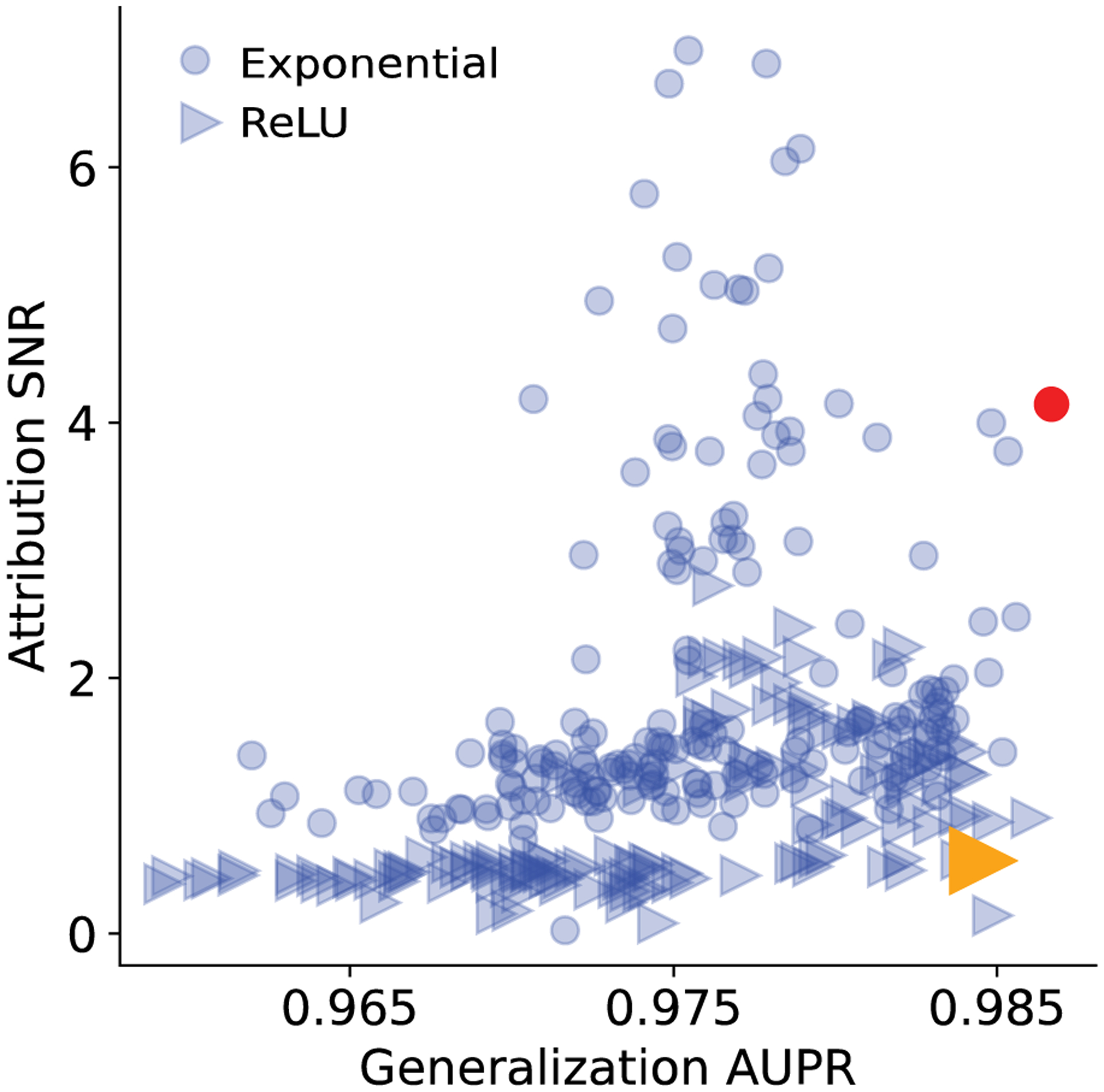
Test performance on synthetic data. Scatter plot of area-under the precision-recall (AUPR) curve and attribution SNR (based on saliency maps) for various DNNs trained with different regularization methods on synthetic data. Each point represents a different model and the marker represents whether the first layer activation was ReLU or exponential. Annotated points represent 2 DNNs that yield high generalization performance but different attribution SNRs.
Figure 5:
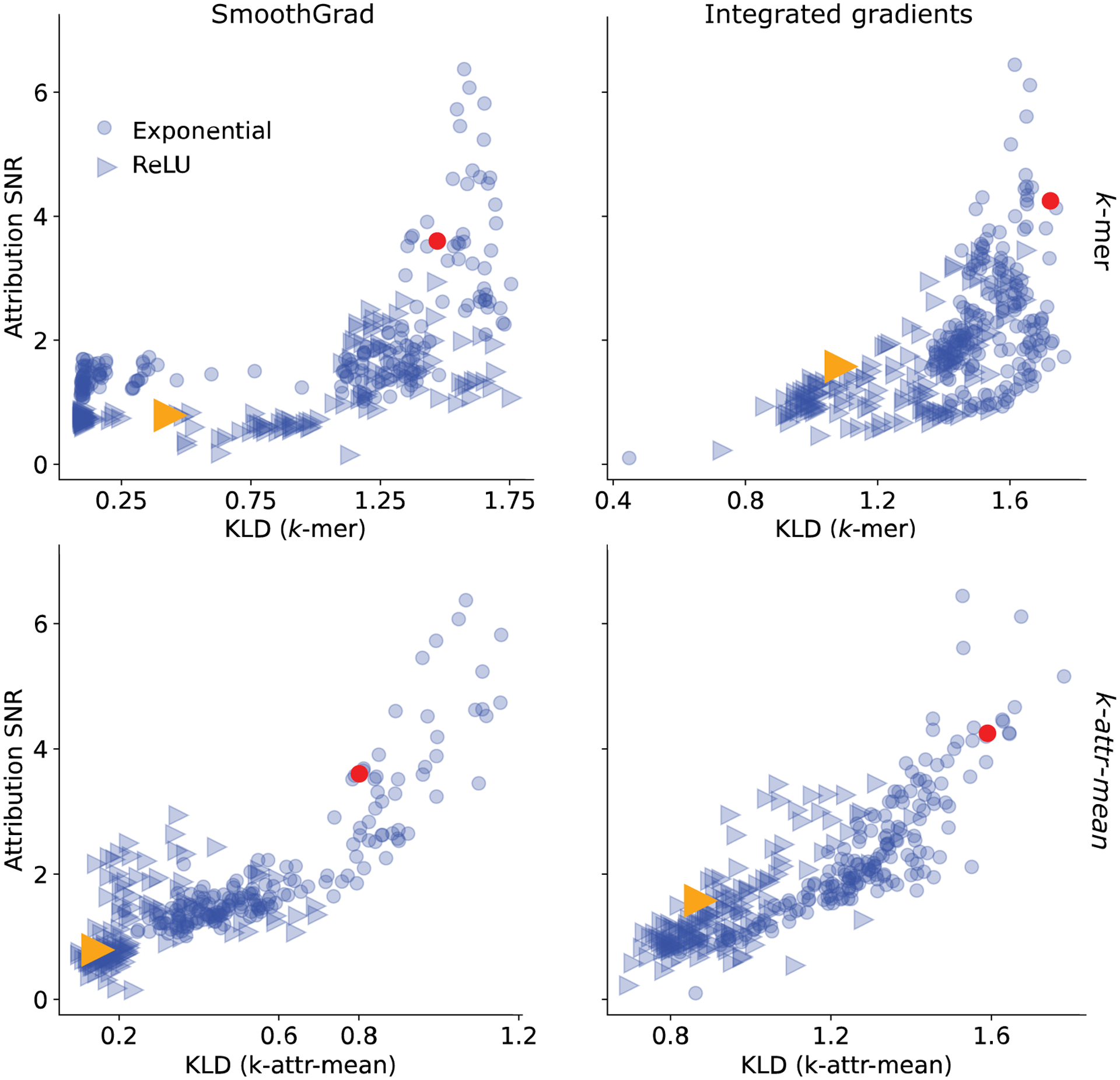
Consistency performance for different attribution methods on test set of synthetic data. Scatter plot of attribution SNR versus the consistency metric of the -mer method (top row) and -attr-mean method (bottom row) for attribution maps based on SmoothGrad (left column) and integrated gradients (right column). Annotated points represent the two DNNs that yield high generalization performance (e.g. AUROC/AUPR) but different attribution SNRs according to saliency maps in Figures 2a–c.
Figure 6:
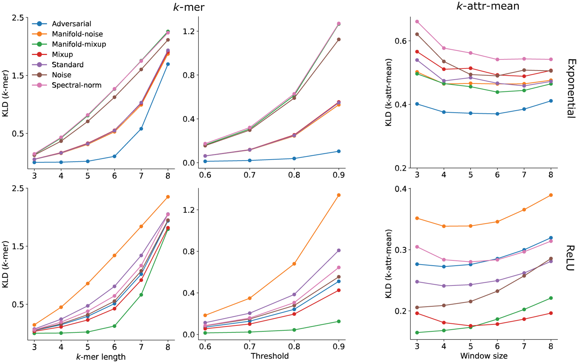
Hyperparameter sensitivity analysis. Sensitivity analysis of hyperparameter choices on the consistency metrics across models with different regularization methods (shown in a different color) averaged across trials, where top row represents models with exponential activations in the first layer and the bottom row represents models with ReLU activations. For the -mer method, hyperparameters of the -mer size (left column) and the attribution threshold (middle column). For the -attr-mean method, the attribution window size was explored. The line serves as a guide for the eye.
Footnotes
Code Availability
Code to reproduce most of the analysis in this paper can be found here:https://github.com/crajesh6/acme.
this is accomplished by simply clipping the argument to .
References
- [1].Kelley David R, Reshef Yakir A, Bileschi Maxwell, Belanger David, McLean Cory Y, and Snoek Jasper. Sequential regulatory activity prediction across chromosomes with convolutional neural networks. Genome Research, 28(5):739–750, 2018. [DOI] [PMC free article] [PubMed] [Google Scholar]
- [2].Maslova Alexandra, Ramirez Ricardo N, Ma Ke, Schmutz Hugo, Wang Chendi, Fox Curtis, Ng Bernard, Benoist Christophe, Mostafavi Sara, et al. Deep learning of immune cell differentiation. Proceedings of the National Academy of Sciences, 117(41):25655–25666, 2020. [DOI] [PMC free article] [PubMed] [Google Scholar]
- [3].Avsec Žiga, Agarwal Vikram, Visentin Daniel, Ledsam Joseph R, Grabska-Barwinska Agnieszka, Taylor Kyle R, Assael Yannis, Jumper John, Kohli Pushmeet, and Kelley David R. Effective gene expression prediction from sequence by integrating long-range interactions. Nature Methods, 18(10):1196–1203, 2021. [DOI] [PMC free article] [PubMed] [Google Scholar]
- [4].Karbalayghareh Alireza, Sahin Merve, and Leslie Christina S. Chromatin interaction-aware gene regulatory modeling with graph attention networks. Genome Research, 32(5):930–944, 2022. [DOI] [PMC free article] [PubMed] [Google Scholar]
- [5].Chen Kathleen M, Wong Aaron K, Troyanskaya Olga G, and Zhou Jian. A sequence-based global map of regulatory activity for deciphering human genetics. Nature Genetics, 54(7):940–949,2022. [DOI] [PMC free article] [PubMed] [Google Scholar]
- [6].Inukai Sachi, Kock Kian Hong, and Bulyk Martha L. Transcription factor-dna binding: beyond binding site motifs. Current Opinion in Genetics & Development, 43:110–119, 2017. [DOI] [PMC free article] [PubMed] [Google Scholar]
- [7].Koo Peter K and Ploenzke Matt. Deep learning for inferring transcription factor binding sites. Current Opinion in Systems Biology, 2020. [DOI] [PMC free article] [PubMed] [Google Scholar]
- [8].Novakovsky G, Dexter N, Libbrecht MW, Wasserman WW, and Mostafavi S. Obtaining genetics insights from deep learning via explainable artificial intelligence. Nature Reviews Genetics, 2022. [DOI] [PubMed] [Google Scholar]
- [9].Simonyan Karen, Vedaldi Andrea, and Zisserman Andrew. Deep inside convolutional networks: Visualising image classification models and saliency maps. arXiv:1312.6034, 2013. [Google Scholar]
- [10].Sundararajan Mukund, Taly Ankur, and Yan Qiqi. Axiomatic attribution for deep networks. In International Conference on Machine Learning, pages 3319–3328. PMLR, 2017. [Google Scholar]
- [11].Smilkov Daniel, Thorat Nikhil, Kim Been, Viégas Fernanda, and Wattenberg Martin. Smoothgrad: removing noise by adding noise. arXiv:1706.03825, 2017. [Google Scholar]
- [12].Shrikumar Avanti, Greenside Peyton, and Kundaje Anshul. Learning important features through propagating activation differences. In International Conference on Machine Learning, pages 3145–3153. PMLR, 2017. [Google Scholar]
- [13].Lundberg Scott and Lee Su-In. A unified approach to interpreting model predictions. arXiv: 1705.07874, 2017. [Google Scholar]
- [14].Nair Surag, Shrikumar Avanti, Schreiber Jacob, and Kundaje Anshul. fastism: performant in silico saturation mutagenesis for convolutional neural networks. Bioinformatics, 38(9):23972403, 2022. [DOI] [PMC free article] [PubMed] [Google Scholar]
- [15].Karollus Alexander, Mauermeier Thomas, and Gagneur Julien. Current sequence-based models capture gene expression determinants in promoters but mostly ignore distal enhancers. bioRxiv, 2022. [DOI] [PMC free article] [PubMed] [Google Scholar]
- [16].Atak Zeynep Kalender, Taskiran Ibrahim Ihsan, Demeulemeester Jonas, Flerin Christopher, Mauduit David, Minnoye Liesbeth, Hulselmans Gert, Christiaens Valerie, Ghanem Ghanem Elias, Wouters Jasper, et al. Interpretation of allele-specific chromatin accessibility using cell state-aware deep learning. Genome Research, pages gr-260851, 2021. [DOI] [PMC free article] [PubMed] [Google Scholar]
- [17].Avsec Žiga, Weilert Melanie, Shrikumar Avanti, Krueger Sabrina, Alexandari Amr, Dalal Khyati, Fropf Robin, McAnany Charles, Gagneur Julien, Kundaje Anshul, et al. Base-resolution models of transcription-factor binding reveal soft motif syntax. Nature Genetics, 53(3):354–366, 2021. [DOI] [PMC free article] [PubMed] [Google Scholar]
- [18].de Almeida Bernardo P, Reiter Franziska, Pagani Michaela, and Stark Alexander. Deepstarr predicts enhancer activity from dna sequence and enables the de novo design of synthetic enhancers. Nature Genetics, 54(5):613–624, 2022. [DOI] [PubMed] [Google Scholar]
- [19].Han Tessa, Srinivas Suraj, and Lakkaraju Himabindu. Which explanation should i choose? a function approximation perspective to characterizing post hoc explanations. arXiv:2206.01254, 2022. [Google Scholar]
- [20].Bartlett Peter L, Long Philip M, Lugosi Gábor, and Tsigler Alexander. Benign overfitting in linear regression. Proceedings of the National Academy of Sciences, 117(48):30063–30070, 2020. [DOI] [PMC free article] [PubMed] [Google Scholar]
- [21].Li Zhu, Zhou Zhi-Hua, and Gretton Arthur. Towards an understanding of benign overfitting in neural networks. arXiv:2106.03212, 2021. [Google Scholar]
- [22].Zhang Chiyuan, Bengio Samy, Hardt Moritz, Recht Benjamin, and Vinyals Oriol. Understanding deep learning (still) requires rethinking generalization. Communications of the ACM, 64(3):107–115, 2021. [Google Scholar]
- [23].Wang Zifan, Wang Haofan, Ramkumar Shakul, Mardziel Piotr, Fredrikson Matt, and Datta Anupam. Smoothed geometry for robust attribution. Advances in Neural Information Processing Systems, 33:13623–13634, 2020. [Google Scholar]
- [24].Alvarez-Melis David and Jaakkola Tommi S. On the robustness of interpretability methods. arXiv:1806.08049, 2018. [Google Scholar]
- [25].Majdandzic Antonio, Rajesh Chandana, and Koo Peter K.. Correcting gradient-based interpretations of deep neural networks for genomics. bioRxiv, 490102, 2022. [DOI] [PMC free article] [PubMed] [Google Scholar]
- [26].Koo Peter K and Ploenzke Matt. Improving representations of genomic sequence motifs in convolutional networks with exponential activations. Nature Machine Intelligence, 3(3):258–266, 2021. [DOI] [PMC free article] [PubMed] [Google Scholar]
- [27].Zhang Hongyi, Cisse Moustapha, Dauphin Yann N, and Lopez-Paz David. mixup: Beyond empirical risk minimization. arXiv:1710.09412, 2017. [Google Scholar]
- [28].Verma Vikas, Lamb Alex, Beckham Christopher, Najafi Amir, Mitliagkas Ioannis, Lopez-Paz David, and Bengio Yoshua. Manifold mixup: Better representations by interpolating hidden states. In International Conference on Machine Learning, pages 6438–6447. PMLR, 2019. [Google Scholar]
- [29].Cohen Jeremy, Rosenfeld Elan, and Kolter Zico. Certified adversarial robustness via randomized smoothing. In International Conference on Machine Learning, pages 1310–1320. PMLR, 2019. [Google Scholar]
- [30].Yoshida Yuichi and Miyato Takeru. Spectral norm regularization for improving the generalizability of deep learning. arXiv:1705.10941, 2017. [Google Scholar]
- [31].Tareen Ammar and Kinney Justin B. Logomaker: beautiful sequence logos in python. Bioinformatics, 36(7):2272–2274, 2020 [DOI] [PMC free article] [PubMed] [Google Scholar]
- [32].Mathelier Anthony, Fornes Oriol, Arenillas David J, Chen Chih-yu, Denay Grégoire, Lee Jessica, Shi Wenqiang, Shyr Casper, Tan Ge, Worsley-Hunt Rebecca, et al. Jaspar 2016: a major expansion and update of the open-access database of transcription factor binding profiles. Nucleic Acids Research, 44(D1):D110–D115, 2016. [DOI] [PMC free article] [PubMed] [Google Scholar]
- [33].Toneyan Shushan, Tang Ziqi, and Koo Peter K.. Evaluating deep learning for predicting epigenomic profiles. Nature Machine Intelligence, 2022. [DOI] [PMC free article] [PubMed] [Google Scholar]
- [34].Shrikumar Avanti, Tian Katherine, Avsec Žiga, Shcherbina Anna, Banerjee Abhimanyu, Sharmin Mahfuza, Nair Surag, and Kundaje Anshul. Technical note on transcription factor motif discovery from importance scores (tf-modisco) version 0.5. 6.5. arXiv:1811.00416, 2018. [Google Scholar]
- [35].Koo Peter K, Majdandzic Antonio, Ploenzke Matthew, Anand Praveen, and Paul Steffan B. Global importance analysis: An interpretability method to quantify importance of genomic features in deep neural networks. PLoS Computational Biology, 17(5):e1008925, 2021. [DOI] [PMC free article] [PubMed] [Google Scholar]
- [36].Ioffe Sergey and Szegedy Christian. Batch normalization: Accelerating deep network training by reducing internal covariate shift. In International Conference on Machine Learning, pages 448–456. PMLR, 2015. [Google Scholar]
- [37].Srivastava Nitish, Hinton Geoffrey, Krizhevsky Alex, Sutskever Ilya, and Salakhutdinov Ruslan. Dropout: a simple way to prevent neural networks from overfitting. The Journal of Machine Learning Research, 15(1):1929–1958, 2014. [Google Scholar]
- [38].Kingma Diederik P and Ba Jimmy. Adam: A method for stochastic optimization. arXiv:1412.6980, 2014. [Google Scholar]
- [39].Bishop Chris M. Training with noise is equivalent to tikhonov regularization. Neural Computation, 7(1):108–116, 1995. [Google Scholar]
- [40].Szegedy Christian, Zaremba Wojciech, Sutskever Ilya, Bruna Joan, Erhan Dumitru, Good-fellow Ian, and Fergus Rob. Intriguing properties of neural networks. arXiv:1312.6199, 2013. [Google Scholar]
- [41].Bradie Brian. A friendly introduction to numerical analysis. Pearson Education India, 2006. [Google Scholar]