Abstract
Objective:
Alzheimer’s Disease and Related Dementia (ADRD) is growing at alarming rates, putting research and development of diagnostic methods at the forefront of the biomedical research community. Sleep disorder has been proposed as an early sign of Mild Cognitive Impairment (MCI) in Alzheimer’s disease. Although several clinical studies have been conducted to assess sleep and association with early MCI, reliable and efficient algorithms to detect MCI in home-based sleep studies are needed in order to address both healthcare costs and patient discomfort in hospital/lab-based sleep studies.
Methods:
In this paper, an innovative MCI detection method is proposed using an overnight recording of movements associated with sleep combined with advanced signal processing and artificial intelligence. A new diagnostic parameter is introduced which is extracted from the correlation between high frequency, sleeprelated movements and respiratory changes during sleep. The newly defined parameter, Time-Lag (TL), is proposed as a distinguishing criterion that indicates movement stimulation of brainstem respiratory regulation that may modulate hypoxemia risk during sleep and serve as an effective parameter for early detection of MCI in ADRD. By implementing Neural Networks (NN) and Kernel algorithms with choosing TL as the principle component in MCI detection, high sensitivity (86.75% for NN and 65% for Kernel method), specificity (89.25% and 100%), and accuracy (88% and 82.5%) have been achieved.
Keywords: Alzheimer’s Disease, Kernel estimation, Mild Cognitive Impairment, Neural Network, Respiratory changes, Sleep Movements
I. Introduction
Alzheimer’s disease diagnostics is at the forefront of biomedical research. An estimated 5.8 million Americans of all ages have Alzheimer’s disease [1], [2]. Between the years 2000 and 2017, deaths from heart disease have decreased 9% while deaths from Alzheimer’s disease have increased 145% [3], [4]. Alzheimer’s disease has no cure and treatments have not emerged although many promising therapeutic clinical trials are in progress. Hence, early and accurate detection and diagnosis are crucial to develop a care plan that may potentially cure or delay some symptoms. Alzheimer’s disease in early stages (i.e. MCI, Mild Cognitive Impairment) typically begins as much as a decade or more before symptoms appear creating the opportunity for earlier treatment options.
There is a strong relation between sleep disorders and neurological status [5]–[7]. Sleep loss from sleep disorders is associated with hemodynamic and autonomic cardiovascular dysregulation, altered inflammatory response and impaired endothelial function [8]. Fragmented sleep results in the impairment of cognitive function and disrupts autonomic nervous system regulatory processes during sleep periods [9], [10]. MCI-related sleep fragmentation has been reported in several studies suggesting that consequent sleep loss may contribute to the development of MCI in its early stages [11], [12]. Yet, the lack of a definitive algorithm or any clearly measurable parameter to assist in diagnostics is strongly felt. In-hospital sleep studies utilize EEG (electroencephalography) or polysomnography as the gold standard of determining sleep states, arousals, and sleep quality. Many non-EEG signals are also used to characterize sleep disorder, e.g. eye and body movements, respiratory frequency/volume, cardiac variability, etc. The advancement of technology specifically in the sensor networks field have improved digital and statistical applications to these measures for home studies [13], [14]. In bio-engineering systems using smartphone applications, wearable tools, such as smart watches, rings or headbands can record and track some relevant sleep parameters [15]–[20]. Parameters related to sleep duration and quality are measured, but no correlation between these parameters and ADRD diagnosis has been reported. Although sleep-wake can be detected by wearables [21]–[29], determining sleep quality (poor sleep or sleep fragmentation) is challenging. EEG, also, is the gold standard for determining sleep and arousal states in sleep studies [30], [31], but EEG is very difficult to record in the home. Hence, to acquire high quality medical-level sleep data in the home that is also most comfortable for the patient is greatly needed.
Our innovation focuses on sleep disorder status, a known hallmark of neurological disease, and commonly present in MCI/AD. Sleep disorder is associated with sleep deprivation (SD) from chronic sleep fragmentation or wake after sleep onset [WASO], poor sleep quality, etc. which over time induce clinically significant daytime cognitive decline. Our sensor system provides standard actigraphy-type sleep fragmentation indices with the value proposition that SleepMove™ mattress platform identifies high frequency, sleep-related movement arousals (i.e. no EEG change, [MA]) [32], [33]. As part of arousal neurocircuitry, MAs are deficient in sleep disorder and neurological disease. It is known that SD suppresses the arousal system during sleep.
In our study, sleep quality is assessed by evaluating sleep movements (SM), or movement arousals, a normal, periodic process (circa 1-3 min) that occurs during sleep studied extensively by our and other groups. Robustness (amplitude/duration) of SM is suppressed during poor sleep quality or sleep loss, and we hypothesize that the coupling with respiratory frequency will be impaired. In our experiments we have used a SleepMove™ device which provides new technology for home recordings of respiratory and movement parameters during sleep without direct contact with the body [32], [33]. This addresses the need to have high quality medical recordings without the use of uncomfortable probes as in hospital studies. Aging patients that complain of sleep problems to the primary care provider may be scheduled for a sleep study from a Neurology group. That sleep study may be a home study in which a wrist actigraph is attached for 24 hours over a period of 2 weeks or more. Alternatively, the patient may receive an in-hospital sleep study for one overnight sleep. In both cases, devices and probes are used to monitor sleep and can be disruptive to sleep continuity. This has the feature of not disrupting sleep in aging persons with sleep disorder. Furthermore, wearable devices can only provide a single point measurement, while SleepMove™ device captures movement and respiratory at 32 points and provides a much higher accuracy when it comes to low signal to noise ratio signals. The SleepMove™ device is an in-home system that makes sleeping in a more comfortable environment possible, while providing an accurate assessment of sleep movements intensity and relative timings as well as associated respiratory signals, while keeping the costs very low. In this work small and large scale body movements over time, including amplitude or intensity of movement and relative timing between these movements coupled with associated respiratory changes are the signals that are measured by the SleepMove™ device over time. Our innovation in this paper is processing the recorded SleepMove™ signals by accurate algorithms and extract useful indices for MCI detection.
This paper presents, for the first time, the processing algorithms of extracting useful features from sleep recorded with the SleepMove™ device, a wireless device commercialized by Activas Diagnostics based on a patent held by the University of Maine [32], [33]. This device is capable of collecting data from various types of piezoresistive sensors deployed in a network to improve the dynamic range of sensor arrays and satisfy the requirements for feature detection and extraction from the collected neuro-motor signals. The network of extremely thin (1mm) sensors are placed underneath the bedding to allow for a flat and unobtrusive sleep surface. Advanced sheets wireless system design addresses the main challenges that include, sensor sensitivity/selectivity, interference, and most importantly low signal to noise ratios associated with brain research applications. Hardware and software examine movement and respiration variability using a fast-time, neuromotor bout detection algorithm (Bout is defined as length of time from onset of a sleep movement epoch to offset with predefined thresholds for onset and offset).
The information that is extracted from the mattress during sleep (one person with no partner) has been determined to be associated with two parameters: movement arousals and respiratory frequency changes. Arousal events during sleep are transient elevation of the vigilance level due to environmental stimuli or driven by oscillation in spontaneous arousal during the sleep period. The American Sleep Disorder Association (ASDA) proposed EEG and chin muscle tone criteria for > 3 – 10 sec and interrupt sleep epochs, typically lasting for a minimum of 1 minute or longer [34]. Alternatively, spontaneous movement arousals are brief (< 15 sec), do not interrupt sleep state, and occur with a periodicity of 1-4 minutes [35], [36]. Our laboratory has reported that movement arousals are part of arousal neurocircuitry, as are full arousals, and similarly, track sleep loss associated with neurological disease or injury [37], [38].
The hypothesis of this work is that high frequency spontaneous movement arousal vigor (i.e. amplitude and duration measures), and its coupled upregulation of respiration variability, is an indication of sleep and cognitive brain health that may be affected by MCI in ADRD. Discussed herein is the signal processing algorithmic approaches to 1) preprocessing and homogenization of recorded signals, 2) estimating the on-bed time, 3) extracting informative signals from the raw data, 4) extracting important features, and 5) designing the discriminating algorithms for the two groups of subjects; MCI and Normal Control (NC) participants.
The rest of this paper is organized as follows. Section II presents a holistic perspective of methods used for data analysis and feature extraction. Mathematical description and background definitions for each processing step of the whole structure is described in this section. The results of the proposed methods and algorithms based on the real data have been discussed in Sec. III and summarized in Sec. IV. The last part of this manuscript, Sec. V, surveys the open research directions that are the most important to address in the future.
II. Methodology
The dataset is derived from an IRB approved study from the University of Maine examining healthy, aging participants (N=40) between 60-90 years of age recruited in Maine. The SleepMove™ device in this study was installed in the participants’ home bed for two nights continuously recording data. MCI status was determined based on prior MCI diagnosis from the Mood and Memory Center at Northern Light Health (https://northernlighthealth.org). MCI participants (n=20) showed selective deficits on both immediate and delayed verbal memory (Hopkins Verbal Learning Task-Revised; Boston Naming Test; Brief Visual Memory Test-Revised), with retention of performance on cognitive reserve and intelligence measures (AMNART; verbal subtest of the Wechsler Adult Intelligence Test). In three cases, a consensus panel of experts in geriatric psychiatry determined MCI status based on interview, health history and neurocognitive battery performance. Normal Cognition (NC) subjects (NC; n=20) were determined to be normative for age on neurocognitive performance. The demographics of MCI and Normal Cognition (NC) groups are shown in Table I. This table shows the health demographics of the MCI and NC participants. MCI group had poorer scores on the MoCA, a test for MCI, and were modestly higher in socioeconomic status. Our sample identified a non-significant greater number of female cases likely related to the greater prevalence of this condition in females.
TABLE I:
Demographics of MCI and Normal Cognition (NC) Groups.
| Variable (μ ± SE or % (n)) | NC (n=20) | MCI (n=20) | p-value |
|---|---|---|---|
|
| |||
| Age, y | 72.2±1.6 | 74.3±1.2 | ns |
| Montreal Cognitive Assessment(MoCA) | 26.5±0.4 | 22±0.56 | < 0.001 |
| Female | 85% (17) | 65% (13) | ns |
| Race | 100% (20) | 100% (20) | ns |
| Years of education | 15.6±0.6 | 15.4±0.6 | ns |
| Socioeconomic Status | 2.9±0.23 | 3.6±0.21 | 0.03 |
| Marital Status (% married/partner) | 35% (7) | 55% (11) | ns |
| Body Mass Index (BMl) | 27.7±1.3 | 26.6±1.3 | ns |
| Obstructive sleep apnea (OSA) | 10% (2) | 20% (4) | ns |
| Diabetes | 10% (2) | 20% (4) | ns |
| Cardiovascular disease | 15% (3) | 10% (2) | ns |
| Cerebrovascular disease | 0% (3) | 10% (2) | ns |
| Traumatic brain injury (TBI) | 15% (3) | 10% (2) | ns |
| Hypercholesterolemia | 40% (8) | 35% (7) | ns |
| Hypertension | 30% (6) | 40% (8) | ns |
| Arthritis | 50% (10) | 55% (11) | ns |
| Current depressed mood | 0% (0) | 35% (7) | ns |
Values are shown as % (n) or mean ± SE, and compared by independent samples t-test (continuous variables) or Chi-square test of association (categorical variables). Current depressed mood was by self-report answering the question “Are you currently feeling depressed?”.
A general overview of the operations performed in this paper is shown in Fig. 1, which is described in detail bellow.
Fig. 1:
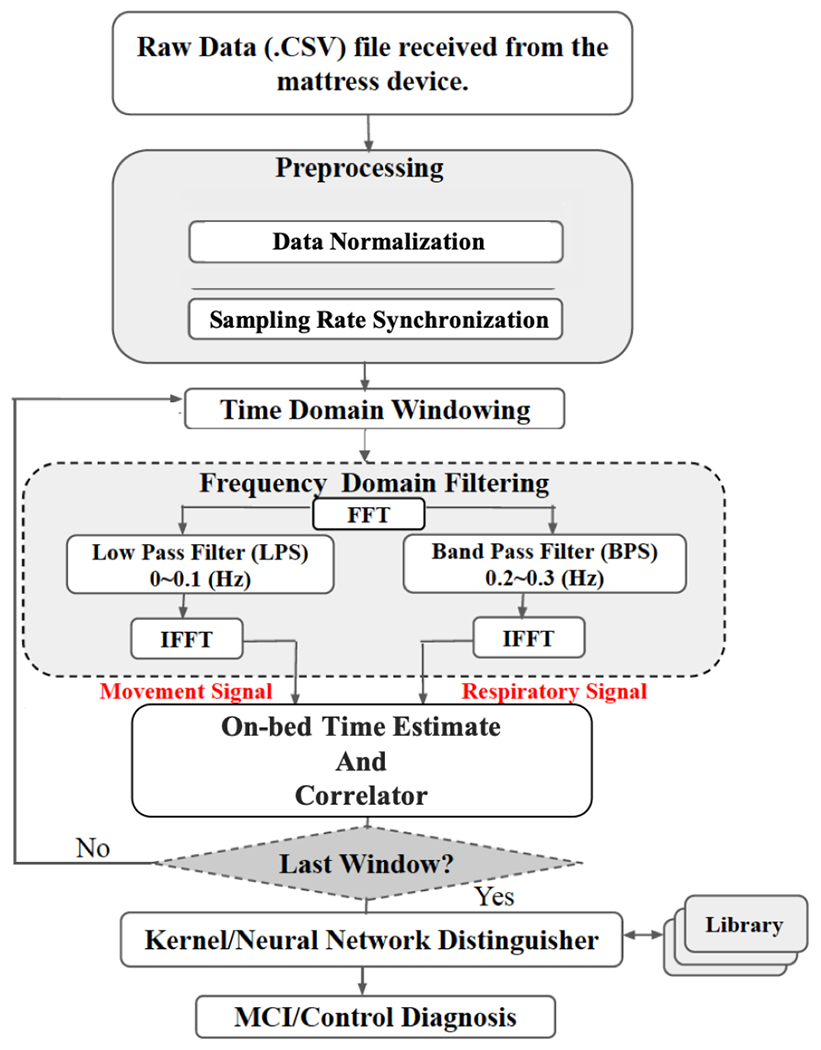
Sleep signal processing flowchart for MCI/NC diagnosis.
A. Preprocessing
Raw data is recorded at a rate of 16 samples per second via 32 channels (16 one-lb and 16 fifty-lb sensors which are switched only when one-lb sensors are saturated). The data matrix, therefore, includes 16 columns each one related to each channel (one of the 1 or 50 lbs sensor pairs records in each time slot).
The first preprocessing operation is normalizing the maximum data amplitudes among all sensors to 1 . This normalization is important to have a fair comparison among sleep signals collected from subjects with different weights/physiological characteristics. A sample of raw signals recorded from 2 sensors during one night can be seen at Fig. 2, where the y-axis is the amplitude of body movements and x-axis shows the time of recording. As shown in Fig. 2, depending on the position of the body during sleep, different sensors record body movement signals from different regions of the body. Sampling rate synchronization (based on upsampling and interpolation) is also done in this step among all sensors to ensure that all sensors’ data are collected with the same sampling rate. Noise remover function is applied in an algorithm during the filtering process in the frequency domain with Movement/Respiratory signals extraction. The Base Algorithm includes filtering and extracting Movement (Mov) and Respiratory (Resp) signals, which is explained in Sec. II-B.
Fig. 2:
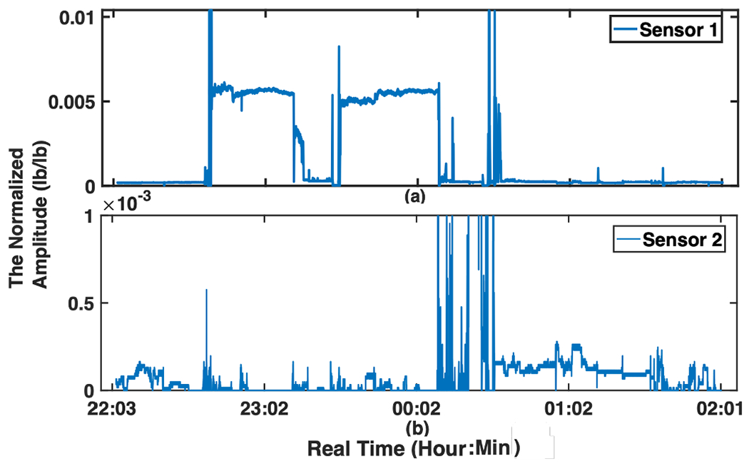
A sample of the raw body movement signal recorded from 2 sensors (sub-figures (a) and (b)) during one night, the y-axes are the normalized amplitude (lb/lb) of the sleep signal (body movements) and x-axis show the time of recording.
B. The Main Algorithm
This section addresses three overarching themes: Extracting all Mov and Resp signals, finding a pattern that shows the relationship between these two signals, and using this pattern to detect ADRD in early stages.
To accomplish these goals, two separate processing algorithms are used.
Time Domain Windowing:
The whole two nights data are separated into minutes epochs with minutes overlaps . This window size is chosen based on the number of sleep-related spontaneous movements with a periodicity of 3-5 minutes, yielding 2-3 events in each 10-min epoch [39].
Frequency Domain Filtering:
The signal of each epoch is then passed through a Fast Fourier Transform (FFT), a Low Pass Filter (LPF), and a Band Pass Filter (BPF). The LPF is designed to extract Mov signal with bandwidth 0-0.1 Hz, since high frequency sleep movements occur about 13 times per hour. There was significant variability in the activity level across participants. A BPF extracts Resp signal with bandwidth 0.2-0.3 Hz, which comprises the respiratory rate per minute based on the number of breaths. Normal respiration rate for an adult at rest is 12 to 20 breaths per minute. Removing higher frequencies removes the noise from the signal, at the same time. An Inverse FFT (IFFT) filter, then gives the time variant Mov/Resp signals to be analyzed. A sample of separated Mov/Resp signals for a duration of 50 minutes is shown in Fig. 3.
Fig. 3:
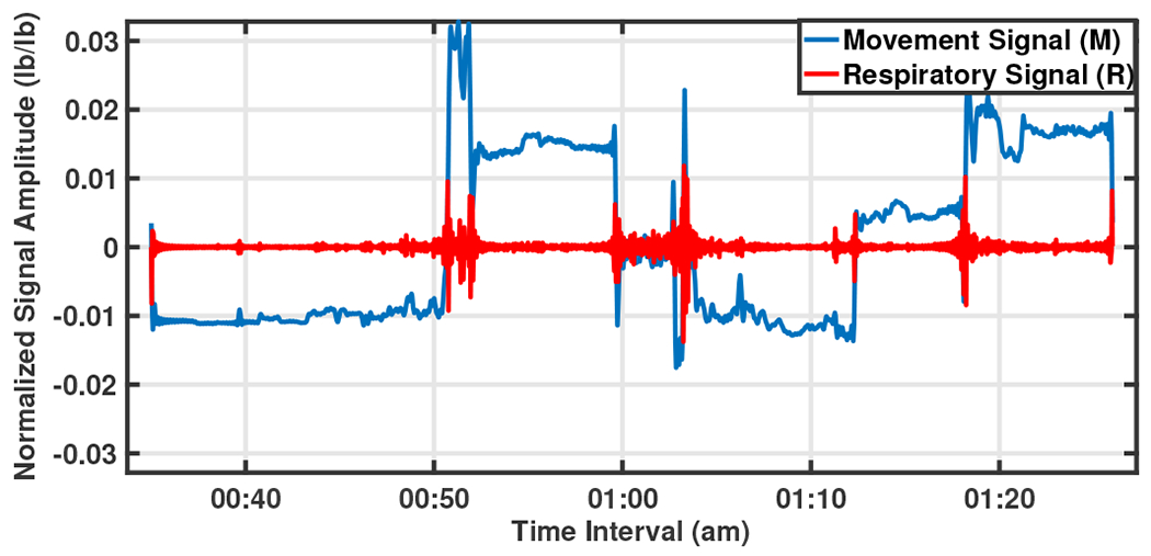
A sample of separated Mov/Resp signals of 50 minutes from 0:35 am to 1:25 am.
In the sequel, in Sec. II-C the algorithm of estimating the accurate on-bed time is explained. This step can be performed before or after the filtering operation, and its purpose is to avoid processing time windows that the bed is not in use. Afterwards, the important features that can be extracted from Mov/Resp signals will be defined in Sec. II-D, while in Sec. II-E we will prove that only 1 of these features is accurate enough to diagnose ADRD based on sleep monitoring. Section II-F introduces the designed diagnosing algorithms based on Neural Network, and the implementation results of which will be discussed in Sec. III. As mentioned before, the entire flowchart of the algorithm shown in Fig. 1 makes it easier to follow the processing stages.
C. On-bed Time Estimation
When the bed is not in use, all sensors measure almost zero pressure, while when the bed is in use, some sensors measure some positive pressure, therefore, an energy threshold is applied to detect the on-bed time. This threshold level of the energy of the signal is considered based on the Power Spectral Density (PSD) metric. For a desired signal with Fourier Transform , PSD can be calculated as,
| (1) |
The energy is computed for -minute windows. If the energy is higher than a predefined threshold chosen empirically, the processing algorithm is started; otherwise, this window will be skipped. It is worth noting that the signal has been normalized to maximum amplitude of 1 and therefore this threshold will be equal for all the subjects. Fig. 4 illustrates the amplitude, the Continuous Wavelet Transform (CWT), and the PSD, in a 10-minute window. Sub-figures (a), (b) illustrate a sample of the recorded signal for the period in which the subject has not used the mattress, while a jump in signal amplitude indicated in sub-figures (d), (e) show the beginning of On-bed time between 10 pm -10:10 pm. Sub-figure (c) also represents the notable difference in energy levels (PSD) of these two sample 10-minute windows which their sub-areas is considered in this paper to be compared with the pre-defined threshold for detecting the on-bed times. By looking at sub-figure (f) which shows the entire recorded signal during the first night, one can clearly see the noticeable change in signal amplitude when using or not using the bed. As this sub-figure shows, this person had gotten out of bed for a couple of hours during the night (from around 0:30 am to 3 am) and laid down again at approximately 7 am.
Fig. 4:
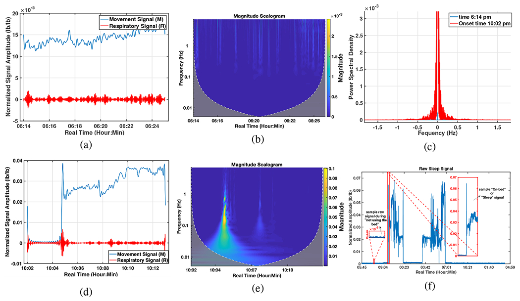
On-bed periods estimation; (a) The mean (among 16 sensors) amplitude, 6:14-6:24 pm., (b) CWT analysis, 6:14-6:24 pm., (c) Comparing the PSDs for two windows before and after laying on the mattress, (d) The mean amplitude, 10:02-10:13 pm., (e) CWT analysis, 10:02-10:14 pm., (f) The whole raw signal (during “not using the bed” and “On-bed” times) recorded over the first night.
Therefore, the time of using the mattress is first extracted and the study is focused on these periods. In this study, the threshold is defined as 0.1% of the maximum energy among all windows during 48 hours. This level is chosen based on comparing the Wavelet illustration of the signal, the mean Amplitude, and the PSD of the signal in different windows. Fig. 5 shows how continuously the mattress is used by two participants for two nights as examples. The windows with the energy higher (or lower) than the threshold are scored 1 (or 0).
Fig. 5:
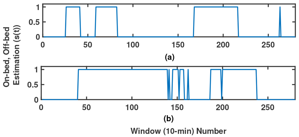
A sample illustration of the on-bed periods of 2 participants (sub-figures (a)-(b), respectively) during two nights. 0-1 signal shows Off-On bed estimation, respectively.
The validation for choosing this threshold is done based on the lab experiments for quality control.
D. Correlator
Aiming to devise a discriminating algorithm to diagnose ADRD participants from the NC group, this section presents 7 features that correlate with neurocognitive status.
Time-Lag (TL) Index Study:
Movements induce physiological upregulation of cardiorespiratory rate that supports homeostasis. This process may be indexed by respiratory rate change although to the best of our knowledge, measuring sleep movements and respiration in time series has not been studied extensively to date. In preliminary work, we have observed that one of these two signals (Mov and Resp) leads the other one [40], as observed in animal studies, movement stimulation increases the rate and tidal volume of the respiratory cycle [41]. Thus, how these two signals correlate can reflect brain function. For this reason, the first analysis tracks the changes in these two signals to examine how Mov and Resp signals affect each other, and the correlation between them is calculated (this operation is done by the Correlator in Fig. 1). In general, correlation describes the mutual relationship between two or more signals. The cross-correlation between signals and , is defined as,
| (2) |
The cross-correlation of the two signals, , is maximum at the time that equals time-lag . For example, consider two similar signals and in Fig. 6 where the first one follows the second signal with variable latency. The sampling rate of these two signals are and their cross-correlation signal ’s maximum value happens at called time-lag. This time shows the time latency between and and the negative sign shows that happens later that . In Fig. 3 such a relation between the Mov and Resp changes is clearly seen, showing that the rate of changes of the two signals is quite similar. It is worthwhile to know the statistical behavior of this time-lag parameter between Mov and Resp signals, e.g. is there any specific range for this parameter in normal aging subjects vs. those with MCI diagnosis? It was hypothesized that there is a distinctive range-based time-lag pattern that is different between NC and MCI participants. To answer these questions, we recorded the between Mov and Resp signals of all 16 sensor pairs, for all -minute epochs during sleep based on the cross-correlation. A sample of three 10-minute epochs illustrating the separated Resp and Mov signals, as well as, their correlation signal and their is shown in Fig. 7 between 10:06 pm to 10:34 pm. With the same procedure, values of all epochs for the two nights was recorded. Therefore, considering minutes epochs with minute overlapping, for two nights of recorded signal (almost 2880 minutes) there are approximately data (280 epochs and 16 sensors) recorded for each participant.
Fig. 6:
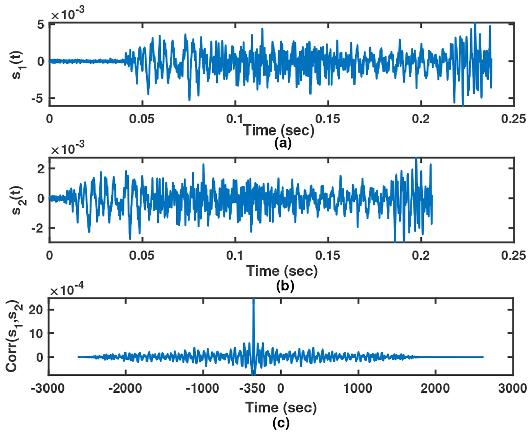
A simple example of the cross-correlation between two sample signals (sub-figure (a)), (sub-figure (b)) and their cross-correlation (sub-figure (c)) with sampling rate .
Fig. 7:
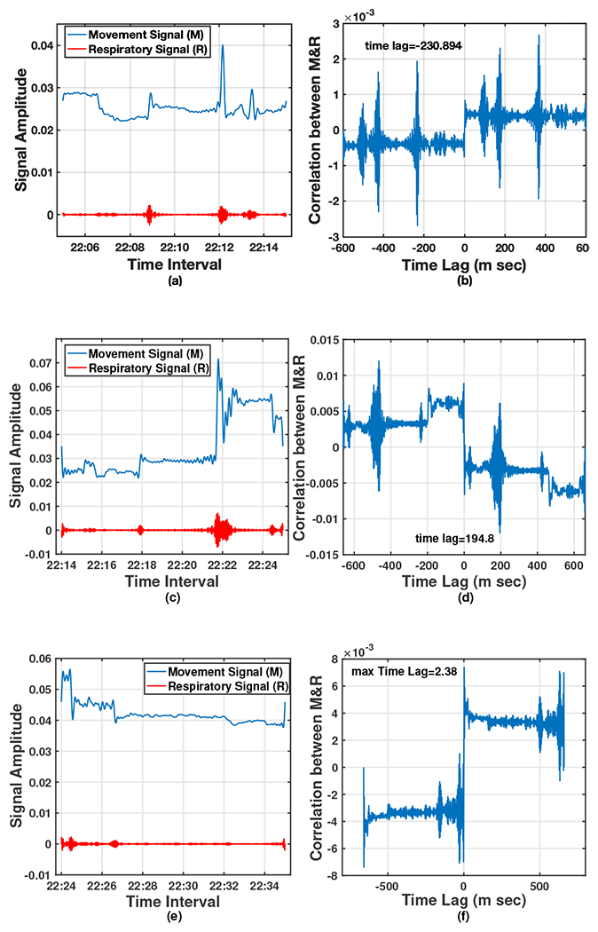
A sample of three 10-minute epochs; (a), (c), (e): separated Resp and Mov signals, and (b), (d), (f): their corresponding correlation signal and the time lag.
In the meantime, considering that at each time slot each sensor senses different levels of pressure, some sensors recorded stronger signals and some very weak signals. With this in mind, for dedicating a Time-Lag quantity as an Index, a calculation is done by giving a weight value to each based on the power of each sensor’s sensed signal and then the average of all weighted among all epochs is considered as follows,
| (3) |
where, is the number of effective epochs during two nights for participant , and is the power of signal sensed by sensor at epoch . Fig. 8 as a sample illustrates the TL histograms for three different participants in two nights sleep monitoring.
Fig. 8:
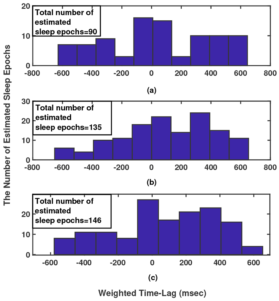
The time-lag histogram between Resp and Mov signals in 280, 10-minute epochs during 2 nights for three participants.
Sleep Duration and Fragmentation Estimates:
As explained in Sec. II-C a time series of 0-1 is extracted for each subject showing an estimation of the time on-bed. We used this time series to calculate two other parameters related to classification into the MCI vs. the NC groups. One is the duration of laying on the mattress (summation of 1s), a parameter related to the sleep duration (SD) in two nights, and the other parameter is related to sleep fragmentation (SF). Both parameters can be calculated by transferring this extracted 0-1 time series to the frequency domain using FFT. The first frequency component (zero frequency component) is the DC value of the signal illustrating the value of SD. The amplitude ratio of the second frequency component to that of zero (DC) has been used as a measure of SF. With increased variation in on-bed to on-bed timing, the power near the fundamental frequency (the second frequency component) spreads across adjacent frequencies, causing a widening and decrease in peak height. The smaller this value vs. the DC shows the person has had a more constant and less fragmented sleep (on-bed time). Fig. 9 shows the frequency domain display (FFT) of sample time series for two different subjects which have been illustrated in Fig.5. (Note: Extracting the sleep stages (Wake, Sleep (N1, N2, N3, and R which are the different phases of sleep based on sleep EEG parameters, [26], [27], [42])) is not the aim of this paper.)
Fig. 9:
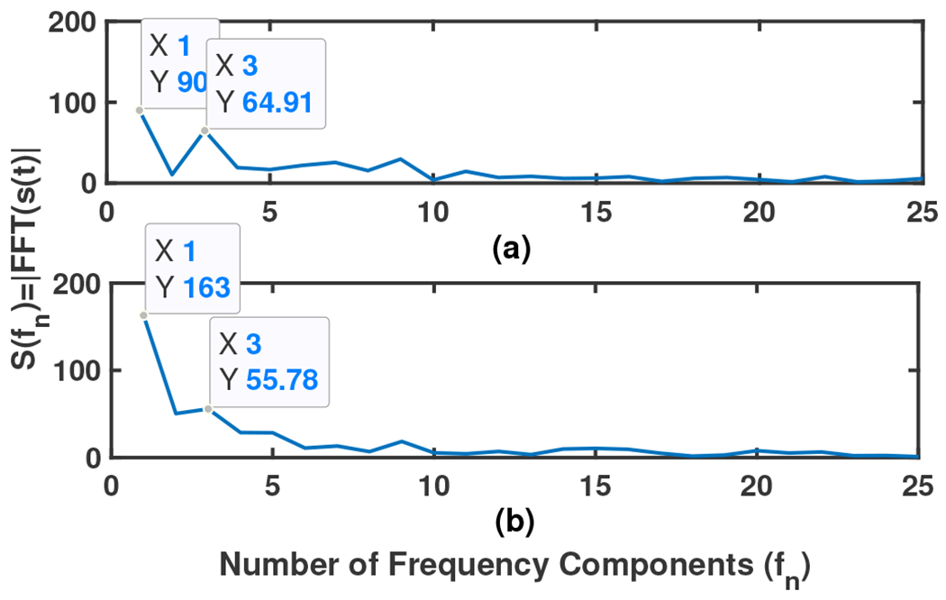
Frequency domain display of sample time series in Fig. 5
Maximum Amplitude, Age and Weight:
Three other features that are selected and can be relevant to the subjects’ cognitive performance are the Maximum Amplitude, Age and Weight of the subjects. As it is explained in Subsection II-A all recorded signals’ amplitude from different subjects are normalized to one for the sake of a fair comparison. However, to not lose any information which can be important for categorizing subjects, the maximum amplitude of each signal is considered as a separate feature.
E. Principle Directions and Dimensionality Reduction
After defining the upper mentioned features, knowing how much each feature is related to early detection of MCI in ADRD would be very useful and practical. Supervised Principal Components Analysis (PCA) using Singular Value Decomposition (SVD) [43], [44] can score the features and reduce the dimensionality of the feature matrix. Our feature matrix is with size , where 7 is the number of features, mean of weighted TL, variance of weighted TL, sleep duration component, sleep fragmentation component, maximum Amplitude of the signal, age, and weight, respectively. We first define a new standardized data matrix with zero mean and variance along each dimension 1, by subtracting the mean from and dividing the standard deviation of each row by each row, then compute the covariance matrix which is a matrix [44],
| (4) |
| (5) |
SVD decomposition of now gives us the singular values of where we can show by choosing dimension (features) how much accuracy can be achieved. Consider the complete SVD of as,
| (6) |
where, is a unitary matrix, is a diagonal matrix and its diagonal elements are the eigenvalues of . The eigenvalues define the magnitude of the principle components. The results of SVD of for our feature matrix are,
| (7) |
As a measure of the achievable Accuracy of designing a network using dimension feature matrix, Total Explained variance (the percentage of variance that is attributed by each of the selected components) is used to measure the discrepancy between a model and actual data [44],
| (8) |
where, considering the values of vector in (7), for in (8) which is totally acceptable for this study. This result show the feature of the mean weighted Time-Lag alone can train the network optimally, and adding other features, or using them separately to train the network will cause more distraction and error in the outcome.
Another confirmation of the veracity of this claim will be discussed later in Sec. III.
F. Devising The Neural Network
Neural networks offer specific advantages such as being adaptive with less formal statistical training, the ability to implicitly extract complex nonlinear functions if they exist between dependent and/or independent variables, the ability to find all interactions may happen among estimator variables, and the availability of different training algorithms. As the schematic in Fig. 10 illustrates, a neural network is composed of an input layer, an output layer, and some hidden layers in between (note: designing more than 2 layers converts Neural Network to Deep Learning). Each layer consists of a bunch of nodes which are symbols of the data features and are connected to the nodes of the next layer by some weighted links. The output of each layer is calculated based on a summation of weighted input data and the transfer functions (Unit step (threshold), sigmoid, piecewise linear, and Gaussian are commonly used [44]) and will be passed to the next layer.
Fig. 10:
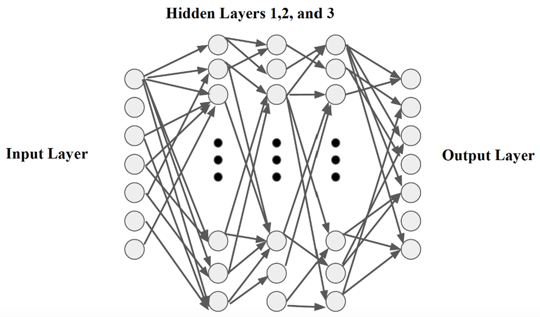
Schematic structure of a sample Neural Network
A two-layer feed-forward backpropagation network is devised in this study and tested. We use “trainlm” in MATLAB simulation as a network training function that updates weight and bias values according to Levenberg-Marquardt optimization. trainlm is often the fastest backpropagation algorithm in the toolbox, and is highly recommended as a first-choice supervised algorithm. The loss function is chosen as Mean Square Error (MSE). Also, due to the low number of unique datasets (40 participants in total) compared to what is common for Neural Network training, the batch size is considered to be equal to the number of samples, and the Leave-One-Out Cross Validation (LOOCV) method is used to train and test the network [44]. A feed-forward neural network is categorized in the group of logistic regression models accumulated on top of each other, where the last layer can be either logistic regression or a linear regression model, depending on the problem which is a classification or regression model [44]. The mathematical interpretation of the input, output and the weighted links for a two-layer trained Neural Network (that is used in our implementation) can be written as,
| (9) |
where, is the input data matrix or feature matrix is the size of the feature vector and is the number of the subjects), is the links’ weight matrix of layer while is the chosen number of neurons, is the constant vector adding to the weighted summation of the inputs to the layer is the transfer function as explained previously, where we used the Sigmoid function with learning rate equal to 0.01 which showed a better LOOCV result, and (.)T shows the transpose of a matrix.
Theoretically, all information about the data as the feature vector can be used to train a neural network and some features which are not useful or relevant to reach the output will get weaker weights after the network is trained. However, we may need a large number of neurons or layers (going to deep learning with more than 2 layers) to get accurate results. As we are not sure which of the defined and extracted features can inherently be useful to diagnose MCI and NC subjects and for the sake of avoiding high complexity in the trained network we trained different networks using different sizes (from one by one feature to all together) of the feature vector, each time the performance of the trained network evaluated based on LOOCV and comparing the results of all networks the features which had a distracting effect on the performance have been removed from the feature vector. This procedure was repeated until satisfaction with the Sensitivity, Specificity, and Accuracy was achieved. Sensitivity, Specificity, and Accuracy parameters are defined as probability that a test result will be negative when ADRD is not present and the subject is in NC group, probability that a test result will be positive when ADRD is present and the subject is in MCI group, and the probability that a test result is true considering the test data is ADRD (positive) or NC (negative), respectively. These parameters can be calculated as,
| (10) |
| (11) |
| (12) |
where, TN (True Negative)/TP (True Positive) is the number of NC/MCI subjects that are correctly detected, and FN (False Negative)/FP (False Positive) is the number of MCI/NC subjects that are wrongly diagnosed by the discriminating algorithm. The Monte Carlo simulation results of the Neural Network-based discriminating algorithm’s implementation is discussed in Sec. III-B.
III. Results And Discussion
This section provides the result of processing data recorded from 16 sensor pairs during two nights of study while the sensors monitored all weak and strong body motions with the sampling rate of 16 Hz. The preprocessing operations, i.e. synchronizing the sampling rate, amplitude normalization, and removing the time windows that the mattress has not been used from the processing algorithm, are done as explained in Sec. II-A and II-C and processing the data and extracting features based on Sec. II-B’s description were conducted. After extracting the aforementioned 7 features, the mean and the variance of Time-Lag, sleep duration and fragmentation, maximum amplitude, age, and weight, for each subject, each feature is examined for utility toward categorizing the subjects into either the MCI or NC group. The histogram display of these 7 features for 40 subjects is shown in Fig.11. This figure gives statistical information of a frequency distribution of each feature, in another word it shows how often each different feature in our set of data occurs. Table II also shows some information of all subjects along with the calculated for each one. In our study -index is calculated for subjects where 20 of them are diagnosed as MCI and 20 as NC based on neurocognitive performance testing and interview. The last column of this table has the result of the designed Neural Network (NN Score) which will be explained later in sub-section III-B. Two discriminating algorithms were applied based on Kernel Density Estimation (KDE), as a second method for comparison, and Neural Networks (NN).
Fig. 11:
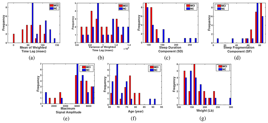
Histogram illustration of (a) The mean of weighted Time Lags, (b) The variance of weighted Time Lags, (c) Sleep duration component, (d) Sleep fragmentation component, (e) Maximum Amplitude of the sleep signal, (f) Age, and (g) Weight.
TABLE II:
Participants Status, TL, and NN Score.
| participant | Sex* | Age | Weight(lb) | Specialist decision | Mean Time Lag (msec) | NN Score** |
|---|---|---|---|---|---|---|
|
| ||||||
| 003 | F | 69 | 130 | NC | 75.5 | −0.97 |
| 005 | F | 68 | 170 | NC | 59.6 | −0.36 |
| 007 | F | 69 | 211 | NC | 116.8 | −0.99 |
| 008 | F | 71 | 245 | NC | 112.4 | −1 |
| 0011 | F | 75 | 156 | NC | 114.56 | −0.99 |
| 0012 | F | 65 | 150 | NC | 62.48 | −1.06 |
| 0016 | F | 70 | 135 | NC | 131.02 | −0.99 |
| 0017 | M | 74 | 180 | NC | 130.07 | −1 |
| 0020 | F | 66 | 139 | NC | 62.42 | −1 |
| 0021 | F | 74 | 190 | NC | 67.27 | −0.98 |
| 0040 | M | 69 | 200 | NC | 71.7 | −0.98 |
| 0047 | F | 74 | 145 | NC | 109.79 | −0.99 |
| 0023 | F | 66 | 135 | NC | 67.91 | −0.98 |
| 0033 | F | 78 | 304 | NC | 147.1 | −1 |
| 0079 | F | 68 | 155 | NC | 111.1 | −1.01 |
| 0083 | F | 65 | 132 | NC | 60.81 | −0.88 |
| 0089 | F | 88 | 122 | NC | 112.45 | −1 |
| 0095 | M | 73 | 188 | NC | 63.66 | −0.98 |
| 0097 | F | 92 | 120 | NC | 64.08 | −0.98 |
| 00100 | F | 69 | 153 | NC | 64.82 | −0.98 |
| 001 | F | 75 | 166 | MCI | 49.5 | 0.98 |
| 002 | F | 67 | 235 | MCI | 103.9 | 0.99 |
| 004 | F | 66 | 125 | MCI | 58.6 | 0.97 |
| 006 | M | 70 | 220 | MCI | 103.6 | 1 |
| 0010 | M | 77 | 159 | MCI | 37.1 | 0.98 |
| 0013 | F | 68 | 198 | MCI | 85.77 | 0.98 |
| 0041 | M | 68 | 202 | MCI | 89.5 | 0.99 |
| 0045 | M | 78 | 137 | MCI | 34.97 | 0.98 |
| 0046 | M | 74 | 145 | MCI | 61.4 | 0.97 |
| 0048 | F | 81 | 158 | MCI | −4.9 | 0.99 |
| 0050 | M | 78 | 178 | MCI | 46.06 | 0.98 |
| 0054 | F | 82 | 230 | MCI | −2.92 | 1 |
| 0084 | F | 82 | 130 | MCI | 99.99 | 1 |
| 0085 | F | 69 | 169 | MCI | 53.8 | 0.98 |
| 0086 | M | 77 | 158 | MCI | 56.01 | 1.04 |
| 0099 | F | 70 | 129 | MCI | 89.18 | 0.99 |
| 00102 | F | 71 | 120 | MCI | 60.04 | 0.35 |
| 00103 | F | 78 | 165 | MCI | 100.63 | 1.01 |
| 00104 | F | 74 | 180 | MCI | 42.74 | 0.98 |
| 00109 | F | 80 | 115 | MCI | 34.25 | 0.98 |
F: Female, M: Male, MCI: Mild Cognitive Impairment, NC: Normal Control
NN Score: Neural Network Score.
KDE is a simple non-parametric density model [44], [45], and in our paper is used to define a probabilistic “Range of Changes” for each feature for each group of subjects. For example, for the TL feature for any real values of , the kernel density estimator’s formula is given by,
| (13) |
where are -indices calculated for each subject, is its Probability Density Function (PDF) estimation, is the number of subjects, is the kernel smoothing function, and is the non-zero positive bandwidth.
Using this function, the PDF estimation for MCI and NC groups for all 7 features has been calculated, separately, and a discriminating algorithm is defined. In the sequel, the results of the processes of the two implemented algorithms are analyzed.
A. KDE Algorithm Results
First, the KDE algorithm outcomes were addressed. This algorithm provides an estimation of the PDF of a random variable. Since it is not known exactly which of the 7 defined parameters can be used as a distinguishing feature, a KDE for each feature was calculated for the two groups of subjects (MCI and NC) shown in Fig. 12.
Fig. 12:
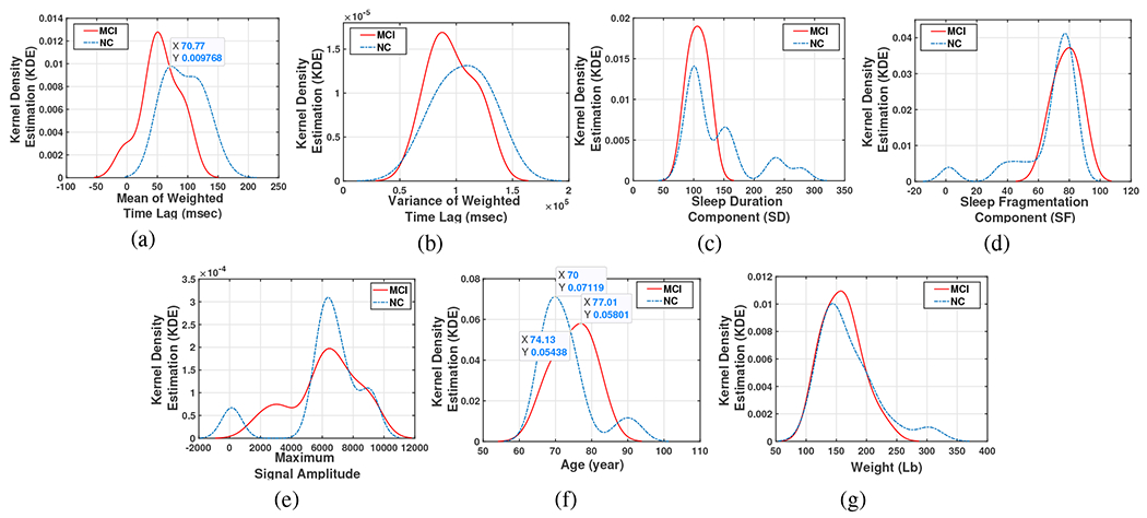
Kernel Density Estimation of (a) The mean of weighted Time Lags, (b) The variance of weighted Time Lags, (c) Sleep duration component, (d) Sleep fragmentation component, (e) Maximum Amplitude of the sleep signal, (f) Age, and (g) Weight.
As it can be seen in this figure, for some of the features, the range of the variations for both groups is almost the same (e.g. (c)-(e) and (g)), and cannot be used alone as a discriminating feature. For example Fig.12-(c) shows that on an average on-bed estimate of sleep duration in two nights for both MCI and NC groups is approximately 1000-1060 minutes (100-106 10-min window) which is about 8-9 hours a day, likewise, the same sleep fragmentation (SF) is seen in both groups as (Fig.12-(d)) shows, however, this parameter on average is somewhat more for MCI group which makes sense. From Fig.12-(f) we see the age average of MCI group (around 85) is also greater than age average in NC group (70).
The mean and the variance of the Time-Lag between Mov and Resp signals show an interesting trend. In Fig.12-(a) (with right/left-tailed p-value for MCI group , and for NC group 0.115/0.17) and 12-(b) (with right/left-tailed p-value for MCI group 0.05/0.08, and for NC group, 0.09/0.084), movement changes caused by respiratory (determined by the TL’s average peak which is positive, hence respiratory change occurs first) shows that in the MCI group, on average, respiratory events precede movement compared to the NC group in which the movement-respiratory coupling sequence is observed . Another striking observation from this figure is that those whose mean TL is less than around 70 msec are more likely to be in MCI group. Hence, the MCI group shows an atypical pattern in which respiratory rate change leads movement arousal response. This pattern is observed during apnea events in which respiratory pauses lead to large movement arousal events that terminate that event. MCI cases have been shown to have a higher risk of apnea diagnosis, although not in the present sample [46]. We hypothesize that the TL reversal in MCI is a new biomarker for MCI risk assessment in this population. Furthermore, the variance of the TL parameter in the NC group is greater than the MCI. Considering these observations we focused on the mean of TL as a discriminating feature.
A cross validation method, LOOCV, used to validate the TL-based KDE algorithm to identify MCI subjects, in such a way that for N subjects we run the algorithm N times. Each time using the TL data of all subjects except one, the TL-based KDE for two MCI and Normal Control subjects is calculated and then the one removed subject was tested. The cross point of the two KDE curves (which can be different for different batches of training data) will determine the test data status. Fig. 13 clarifies the testing process where Fig. 13-a is plotted for all subjects except one (subject 003), which will be considered as the test subject. Now, if the test point sits on the left side with the test subject will be diagnosed as a person with increased probability or risk of MCI, and if the test subject is considered as Normal Control. Based on the position of the test data, the algorithm determined that subject as MCI, while based on Table II, this subject was in the category of NC. Therefore, here there is a False Positive (FP, false diagnosis about an MCI subject) error accrued by the algorithm. Fig. 13-b on the other hand shows a True Negative (TN, true diagnosis about a Normal Control subject) decision for another subject (005) as a Normal Control subject. This process is repeated for all subjects and the number of True or False decisions is counted which can be seen in Table III. In this table, Sensitivity, Specificity, and Accuracy are calculated based on equations (10)–(12). These results indicated which features to use for our next steps in data analysis.
Fig. 13:
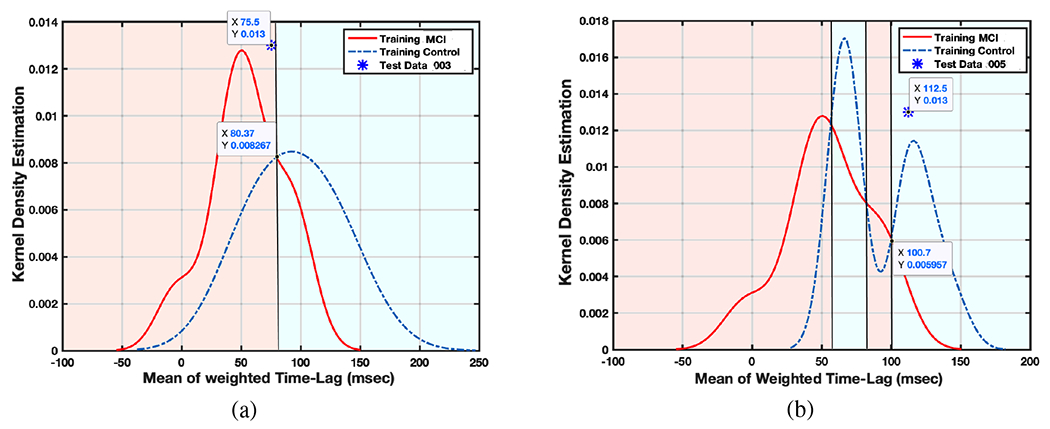
Two sample for LOOCV validation of KDE algorithm
TABLE III:
Leave-Out Cross Validation (LOOCV) Result
| N=40 | KDE | 5 neurons | 10 neurons | 20 neurons |
|---|---|---|---|---|
|
| ||||
| True Positive(out of 20 MCI) | 13 | 13.8 | 16.6 | 17.35 |
| True Negative(out of 20 NC) | 20 | 18 | 18 | 17.85 |
| False Positive(out of 20 NC) | 0 | 2 | 2 | 2.15 |
| False Negative(out of 20 MCI) | 7 | 6.2 | 3.4 | 2.65 |
| Specificity | 100% | 90% | 90% | 89.25% |
| Sensitivity | 65% | 69% | 83% | 86.75% |
| Accuracy | 82.5% | 79.5% | 86.5% | 88% |
B. Neural Network Algorithm Results
Aiming to improve the performance, a Neural Network algorithm is also designed to diagnose ADRD based on sleep monitoring. However, Neural Network has the capability to include all of the features, and through training find the best connection among them to reach the desired output, entering the more dispersed and non-relevant information in this network makes it more complicated and time-consuming. In short, the network will need more neurons and/or more layers in order to reach high performance. For this reason, a trained human intelligence and logic can improve artificial intelligence in the simplest possible way.
Earlier in Sec. II-E we showed that keeping only one feature out of 7 defined features would be enough for training our discriminating algorithms.
With this point in mind, we trained different Neural Networks with one by one features, two by two and so on, until all features together, with different numbers of neurons from 5 to 20 and limited number of layers equals two to avoid complexity. LOOCV is used to evaluate the validity of the algorithm. Again, the results show the feature of mean weighted Time-Lag alone can train the network optimally, and adding other features, or using them separately to train the network will cause more distraction and error in the outcome.
Another confirmation of the veracity of this claim is the regression plot illustration in Fig.14, when we used each feature alone to train a neural network with two classes defined for the output, 1 for the ADRD group and −1 for the NC group. The more distance and the more diversity that data has from the Fit line, shows less correlation and dependency that the neural network could find between the specific data and the output. And, as it can be seen Fig.14-(a) shows a good dependency among all the other features which is related to the mean of weighted Time Lag feature.
Fig. 14:
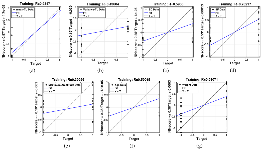
Regression plot of separate neural networks with input data (a) The mean of weighted Time Lags, (b) The variance of weighted Time Lags, (c) Sleep duration component, (d) Sleep fragmentation component, (e) Maximum Amplitude of the sleep signal, (f) Age, and (g) Weight.
Therefore, by including only the first feature LOOCV result for a designed Neural Network with 5, 10 and 20 neurons is exhibited in Fig. 15 where, red and blue stars show MCI and NC test data, respectively, and circles surrounded the test data with False decision in outcome. The input data for this algorithm as mentioned before is the mean of weighted timelag and the output for training data as 1, −1 for MCI or NC subjects, respectively. Therefore, any positive(negative) Neural Network Score (NNS) for the test data is considered as MCI (NC) diagnosis. The result NNS for all the subjects are given in the last column of Table II. Note that each sub-figure of Fig. 15 is the result of time running the algorithm (each time one subject has been left as test data) in which each times’ outcome is held to be illustrated all in one figure.
Fig. 15:

Three samples for LOOCV validation of Neural Network algorithm with a) 5 neurons, b) 10 neurons, and c) 20 neurons. Red and blue stars show MCI and NC test data, respectively, and circles surrounded the test data with false decision in outcome.
Monte Carlo simulations over 20 runs are performed and the average of desired parameters counted as they come in Table III.
IV. Conclusion
This paper proposed an innovative method for Mild Cognitive Impairment (MCI) detection in Alzheimer’s Disease and Related Dementia (ADRD) using an overnight recording of movements associated with sleep combined with advanced signal processing and artificial intelligence. A new diagnostic parameter named Time-Lag (TL) is introduced which is extracted from the correlation between high frequency, sleep-related movements and respiratory changes during sleep. This newly defined parameter, is proposed as a distinguishing criterion that indicates movement stimulation of brainstem respiratory regulation that may modulate hypoxemia risk during sleep and serve as an effective parameter for early detection of MCI in ADRD. As a result, high sensitivity (respectively, 86.75% and 65%), specificity (89.25% and 100%), and accuracy (88% and 82.5%) achieved by implementing Neural Networks and Kernel algorithms with choosing TL as the principle component in MCI detection.
V. Future Directions and Open Areas
Since this paper is the first paper on analyzing SleepMove™ device’s recorded signal and this device is a new patent, more processing on the recorded data are ongoing, and new features/parameters are being defined and extracted in consultation with the physicians and specialists, which can be used as inputs for the designed Neural Networks algorithm. Also, as it is stated in the paper, because of the nature of such studies and experiments, collecting a large dataset of clinically diagnosed MCI and aging participants for a short-term longitudinal study in the home is very difficult. A future direction is to enlarge the dataset. In addition, we know that usually two databases are employed to evaluate the adaptiveness of the proposed method on other databases was not possible for this first study. One other useful expected algorithm is extracting the pattern of the subjects’ body position based on the strength of signals recorded by different sensors. This pattern may be used as another feature to detect different diseases. Also, estimating Sleep Stages (REM, N1, N2, and N3) based on these signals is a very useful and interesting work that can be a turning point in sleep studies.
VI. ACKNOWLEDGMENT
In addition, a thank you to all Activas Diagnostics members, Shahrzad Abedi, Joel Castro, and Ryan Dufour, as the engineering team, and Chris Gilbert and Jessica Aronis as the psychology team who contributed to on this project to build the device, set up the mattress at subjects’ home, and collect data. This project was financially supported by NIH SBIR Phase II award R44AG059536 and Maine Technology Institute (MTI) Commercialization award.
References
- [1].Gaugler J, James B, Johnson T, Marin A, Weuve J, “2019 Alzheimer’s disease facts and figures,” Alzheimers Dement, vol. 15, no. 3,pp. 321–387, 2019. [Google Scholar]
- [2].Hebert LE, Weuve J, Scherr PA, Evans DA, “Alzheimer disease in the United States (2010-2050) estimated using the 2010 Census,” Neurology, vol. 80, no. 19 , pp. 1778–1783, 2013. [DOI] [PMC free article] [PubMed] [Google Scholar]
- [3].U.S. Department of Health and Human Services, Centers for Disease Control and Prevention, National Center for Health Statistics. CDC WONDER online database: About Underlying Cause of Death, 1999–2017. Available at: http://wonder.cdc.gov/ucd-icd10.html. Accessed December 18, 2018.
- [4].Tejada-Vera B Mortality from Alzheimer’s disease in the United States: data for 2000 and 2010, NCHS Data Brief., no. 116, pp. 1–8, 2013 [PubMed] [Google Scholar]
- [5].Wennberg Alexandra M. V. et al. “Sleep Disturbance, Cognitive Decline, and Dementia: A Review”, Seminars in neurology, vol. 37, no. 4, pp. 395–406, 2017. [DOI] [PMC free article] [PubMed] [Google Scholar]
- [6].Petersen RC, Lundt ES, Therneau TM et al. “Predicting progression to mild cognitive impairment”, Ann Neurol, vol. 85, no. 1, pp. 155–160, 2019. [DOI] [PMC free article] [PubMed] [Google Scholar]
- [7].Petersen RC, Ronald C, et al. “Mild cognitive impairment: a concept in evolution”, Journal of internal medicine, vol. 275, no. 3, pp. 214–228, 2014. [DOI] [PMC free article] [PubMed] [Google Scholar]
- [8].Mullington Janet M., et al. :Cardiovascular, Inflammatory, and metabolic consequences of sleep dprivation”, Progress in cardiovascular diseases 51.4 (2009): 294–302. [DOI] [PMC free article] [PubMed] [Google Scholar]
- [9].Medic Goran, et al. “Short- and long-term health consequences of sleep disruption.” Nature and science of sleep, vol. 9, pp. 151–161, 2017 [DOI] [PMC free article] [PubMed] [Google Scholar]
- [10].Gagnon K, Baril AA, Gagnon JF, et al. “Cognitive impairment in obstructive sleep apnea”, Pathol Biol (Paris), vol. 62, no. 5, pp. 233–240, 2014 [DOI] [PubMed] [Google Scholar]
- [11].Wang Chanung, Holtzman, and David M, “Bidirectional relationship between sleep and Alzheimer’s disease: Role of amyloid, tau, and other factors,” Neuropsychopharmacology, vol. 45, no. 1, pp. 104–120, 2020. [DOI] [PMC free article] [PubMed] [Google Scholar]
- [12].Spira Adam P., et al. “Actigraphic sleep duration and fragmentation in older women: associations with performance across cognitive domains”, Pathol Biol (Paris), vol. 62, no. 5, pp. 233–240, 2014. [DOI] [PMC free article] [PubMed] [Google Scholar]
- [13].Rashid RA, Arifin SHS, Rahim MRA, Sarijari MA and Mahalin NH, “Home healthcare via wireless biomedical sensor network,” 2008 IEEE International RF and Microwave Conference, Kuala Lumpur, PP. 511–514, 2008. [Google Scholar]
- [14].Shahbakhti M et al. “Simultaneous Eye Blink Characterization and Elimination From Low-Channel Prefrontal EEG Signals Enhances Driver Drowsiness Detection,” IEEE Journal of Biomedical and Health Informatics, vol. 26, no. 3, pp. 1001–1012, March 2022. [DOI] [PubMed] [Google Scholar]
- [15].Lee Jung-Min et al. “Comparison of Wearable Trackers’ Ability to Estimate Sleep.” International journal of environmental research and public health, vol. 15,no. 6, pp. 1265, 2018. [DOI] [PMC free article] [PubMed] [Google Scholar]
- [16].Cellini N, Buman MP, McDevitt EA, Ricker AA, Mednick SC, “Direct comparison of two actigraphy devices with polysomnographically recorded naps in healthy young adults” Chronobiol. Int, vol. 30, pp. 691–698, 2013. [DOI] [PubMed] [Google Scholar]
- [17].Carney CE, Buysse DJ, Ancoli-Israel S, Edinger JD, Krystal AD, Lichstein KL, Morin CM “The consensus sleep diary: Standardizing prospective sleep self-monitoring“, Sleep, vol. 35, pp. 287–302, 2012. [DOI] [PMC free article] [PubMed] [Google Scholar]
- [18].Meltzer LJ, Walsh CM, Traylor J, Westin AM, “Direct comparison of two new actigraphs and polysomnography in children and adolescents”, Sleep, vol. 35, pp. 159–166, 2012. [DOI] [PMC free article] [PubMed] [Google Scholar]
- [19].Ahn JW, Ku Y, Kim HC, “A Novel Wearable EEG and ECG Recording System for Stress Assessment”, Sensors 2019, vol. 19, 1991. [DOI] [PMC free article] [PubMed] [Google Scholar]
- [20].Lin S-K, Istiqomah, Wang L-C, Lin C-Y and Chiueh H, “An Ultra-Low Power Smart Headband for Real-Time Epileptic Seizure Detection,” IEEE Journal of Translational Engineering in Health and Medicine, vol. 6, pp. 1–10, 2018. [DOI] [PMC free article] [PubMed] [Google Scholar]
- [21].Shambroom JR et al. “Validation of an automated wireless system to monitor sleep in healthy adults,” J. Sleep Res, vol. 21, no. 2, pp. 221–230, 2012. [DOI] [PubMed] [Google Scholar]
- [22].Heinzer R et al. “Prevalence of sleep-disordered breathing in the general population: TheHypnoLaus study,” Lancet RespiratoryMed, vol. 3 , no. 4, pp. 310–318, 2015. . [DOI] [PMC free article] [PubMed] [Google Scholar]
- [23].Kemp B et al. “Analysis of a sleep-dependent neuronal feedback loop: the slow-wave microcontinuity of the EEG,” IEEE Trans. Biomed. Eng, vol. 47, no. 9, pp. 1185–1194, Sep. 2000. [DOI] [PubMed] [Google Scholar]
- [24].Goldberger AL et al. “PhysioBank, PhysioToolkit, and PhysioNet: Components of a new research resource for complex physiologic signals,” Circulation, vol. 101, no. 23, pp. e215–e220, 2000. [DOI] [PubMed] [Google Scholar]
- [25].Cantero JL et al. “Human alpha oscillations in wakefulness, drowsiness period, and REM sleep: different electroencephalographic phenomena within the alpha band,” Neurophysiol. Clinique, vol. 32, no. 1, pp. 54–71, 2002 [DOI] [PubMed] [Google Scholar]
- [26].Lo C-C et al. “Asymmetry and basic pathways in sleep-stage transitions,” Europhys. Lett, vol. 102, no. 1, 2013, Art. no. 10008. [DOI] [PMC free article] [PubMed] [Google Scholar]
- [27].Kang DY, DeYoung PN, Malhotra A, Owens RL and Coleman TP, “A State Space and Density Estimation Framework for Sleep Staging in Obstructive Sleep Apnea,” IEEE Trans. on Biomed. Eng, vol. 65, no. 6, pp. 1201–1212, June 2018. [DOI] [PMC free article] [PubMed] [Google Scholar]
- [28].Chen JC, Espeland MA, Brunner RL, et al. “Sleep duration, cognitive decline, and dementia risk in older women”, Alzheimers Dement, vol. 12 , no. 1, pp. 21–33, 2016 [DOI] [PMC free article] [PubMed] [Google Scholar]
- [29].de Almondes KM, Costa MV, Malloy-Diniz LF, Diniz BS. “Insomnia and risk of dementia in older adults: Systematic review and meta-analysis”, J. Psychiatr Res, vol. 77, pp. 109–115, 2016. [DOI] [PubMed] [Google Scholar]
- [30].Susmakova Kristina. “Human sleep and sleep EEG.” Measurement science review 4.2 (2004): 59–74 [Google Scholar]
- [31].Aeschbach Daniel, and Borbely Alexander A.. “All night dynamics of the human sleep EEG.” Journal of sleep research 2.2 (1993): 70–81 [DOI] [PubMed] [Google Scholar]
- [32].US Patent: Hayes M, and Abedi A, System and method for early detection of mild traumatic brain injury, US20160183861A1, Published 2016.
- [33].US Patent: Hayes M, and Abedi A, System and method for early detection of mild traumatic brain injury, US10244977B2, Published 2019.
- [34].Lopes MC, Marcus CL. “The significance of ASDA arousal in children”, Sleep, vol. 40, no. 8, 2017 [DOI] [PubMed] [Google Scholar]
- [35].Mograss MA, Ducharme FM, Broullette RT. “Movement/Arousals. Description, classification, and relationship to sleep apnea in children”, Am J Crit Care Med., vol. 150, pp. 1690–1696, 1994. [DOI] [PubMed] [Google Scholar]
- [36].Chen H-C, Lin C-M, Lee M-B, et al. “The relationship between pre-sleep arousal and spontaneous arousals from sleep in subjects referred for diagnostic polysomnograms”, J. Chin. Med. Assoc, vol. 74, no. 2, pp. 81–86, 2011 [DOI] [PubMed] [Google Scholar]
- [37].Troese Marcia, Fukumizu Michio, Sallinen Bethany J., et al. “Sleep fragmentation and evidence for sleep debt in alcohol-exposed infants Early Human Development”, Early human development, vol. 84, no. 9, pp. 577–585, 2008. [DOI] [PubMed] [Google Scholar]
- [38].Hayes MJ, Akilesh MR, Fukumizu M, et al. “Apneic preterms and methylxanthines: Arousal deficits, sleep fragmentation and suppressed spontaneous movements”, Journal of Perinatology, vol. 27, no. 12, pp. 782–789, 2007. [DOI] [PubMed] [Google Scholar]
- [39].Wilde-Frenz J, Schulz H, “Rate and Distribution of Body Movements during Sleep in Humans”, Perceptual and Motor Skills, vol. 56, no. 1, pp. 275–283, 1983. [DOI] [PubMed] [Google Scholar]
- [40].Giraudin Aurore, et al. “Intercostal and abdominal respiratory motoneurons in the neonatal rat spinal cord: spatiotemporal organization and responses to limb afferent stimulation”, Journal of neurophysiology, vol 99, no. 5 , pp. 2626–2640, 2008. [DOI] [PubMed] [Google Scholar]
- [41].Potts JT, Rybak IA, Paton JFR, “Respiratory rhythm entrainment by somatic afferent stimulation”, Journal of Neuroscience, vol. 25, no. 8, pp. 1965–1978, 2005. [DOI] [PMC free article] [PubMed] [Google Scholar]
- [42].Wenbin Shi, Pengjian Shang., et al. “A comparison study on stages of sleep: Quantifying multiscale complexity using higher moments on coarse-graining”, Communications in Nonlinear Science and Numerical Simulation, vol. 44, pp. 292–303, 2017. [Google Scholar]
- [43].Ghojogh Benyamin, Crowley Mark, Unsupervised and Supervised Principal Component Analysis: Tutorial, eprint: 1906.03148, 2019. [Google Scholar]
- [44].Murphy Kevin P. Machine Learning: A Probabilistic Perspective. Cambridge, MA: MIT Press, 2012. [Google Scholar]
- [45].Bishop CM, Pattern Recognition and Machine Learning, Berlin, Germany: Springer, 2006 [Google Scholar]
- [46].Bubu M Omonigho, et al. “Obstructive sleep apnea, cognition and Alzheimer’s disease: A systematic review integrating three decades of multidisciplinary research.”, Sleep medicine reviews, vol. 50, 2020. [DOI] [PMC free article] [PubMed] [Google Scholar]


