Estimating and Testing Random Intercept Multilevel Structural Equation Models with Model Implied Instrumental Variables

Abstract

This study develops a new limited information estimator for random intercept Multilevel Structural Equation Models (MSEM). It is based on the Model Implied Instrumental Variable Two-Stage Least Squares (MIIV-2SLS) estimator, which has been shown to be an excellent alternative or supplement to maximum likelihood (ML) in SEMs (Bollen, 1996). We also develop a multilevel overidentification test statistic that applies to equations at the within or between levels. Our Monte Carlo simulation analysis suggests that MIIV-2SLS is more robust than ML to misspecification at within or between levels, performs well given fewer that 100 clusters, and shows that our multilevel overidentification test for equations performs well at both levels of the model.

Introduction

Structural Equation modeling is a general multivariate statistical framework that allows for the modeling of latent variable regressions (Bollen, 1989). Given clustered data such as students nested within classrooms or patients within hospitals, researchers use multilevel structural equation modeling (MSEM) to model latent variables while simultaneously accounting for clustered observations and different levels of effects. Much progress has been made to develop and validate MSEM techniques making the framework more accessible now more than ever (Bentler & Liang, 2003).

The most used estimator in MSEM is maximum likelihood (ML) applied to all levels of the model simultaneously. This is not without reason—ML offers desirable asymptotic properties (e.g., consistency, asymptotic efficiency) for valid models. Despite the flexibility and success of ML for estimating MSEMs, there are potential shortcomings. ML requires strong assumptions such as correct model specification and no excessive multivariate kurtosis (Browne, 1984). If these assumptions are violated, there is no guarantee of consistency, asymptotic efficiency or asymptotic unbiasedness of the ML estimator.

We highlight five primary shortcomings with the usual ML approach. First, given structural misspecification, system-wide estimators such as ML can spread the effects of misspecification across model parameters. The problem of structural specification may be exacerbated by the multilevel nature of MSEMs in the sense that structural misspecification can occur both at the within level and at the between level. Only limited studies focus on the effects of structural misspecification in MSEMs and robust estimation methods, despite that various studies have been devoted to evaluation of model fit and detection of model misspecification. The only two studies of which we are aware are Yuan and Bentler (2007) and Wang and Kim (2017). Yuan and Bentler (2007) pointed out that a misspecified level will affect other correctly specified levels. Hence, they proposed to segregate the multilevel model into single-level models for estimation. In a simulation study, Wang and Kim (2017) investigated the bias caused by a misspecified latent dimension in the multilevel bifactor model. Second, assessing model fit is complicated and often misleading given traditional chi-square based SEM fit statistics (Yuan & Bentler, 2007; Ryu & West, 2009; Ryu, 2014; Hsu, Kwok, Lin, Acosta, 2015). Potential solutions to model fit assessment have been suggested, though these solutions require fitting additional models (See Ryu, 2014) or fitting each level of the model separately and applying corrections (See Yuan & Bentler, 2007). Third, MSEMs estimated with ML can require prohibitively large sample sizes. The current best practice guidance states that 100 clusters should be the minimum level (Hox & Maas, 2004; Julian, 2001; Holtmann, Koch, Lochner, & Eid, 2016). In many fields, it is largely impractical to obtain more than 50 clusters. Fourth, due to model complexity MSEMS are more likely to encounter estimation complications due to lack of convergence (Ryu, 2009). Fifth, underidentification anywhere in the model can prevent estimation. For instance, one could have an adequately identified model at level 2, but if the model is not properly identified at level 1, then the entire system might not be estimable with ML. To illustrate, suppose that our primary interest lies in the level 2 model and that this model is overidentified. But the level 1 model which is only of secondary interest is underidentified due to insufficient number of indicators for a latent variable. The underidentification of the level 1 model would stymie the ML estimation of the level 1 model.

In this paper, we propose and test a novel limited information estimation approach for MSEMs which we expect to alleviate many of the preceding problems. This approach is based on the Model Implied Instrumental Variable, Two-Stage Least Squares (MIIV-2SLS) estimator, which originates from Bollen (1996). In the context of single level SEMs, the principle of MIIV-2SLS has been used in various studies. For example, Bollen, Kolenikov, and Bauldry (2014) proposed the generalized method of moments estimators based on MIIV; Nestler (2014) used the MIIV-2SLS to handle equality constraints in SEM; Nestler (2015a) used the overidentification test for MIIV-2SLS to test latent nonlinear terms in SEM models; Nestler (2015b) proposed the MIIV-2SLS estimator for the growth curve models; Fisher, Gates, and Bollen (2019) applied MIIV-2SLS to dynamic time-series models; Fisher and Bollen (2020) proposed a way to incorporate the mean structures in MIIV-2SLS; Gates, Fisher, and Bollen (2020) applied MIIV-2SLS to group iterative multiple model estimation to search for relations among latent variables.

The MIIV-2SLS approach has been shown to be a useful alternative to ML for estimating single level SEMs (Bollen, 2019). MIIV-2SLS provides solutions for each of the ML shortcomings. First, MIIV-2SLS has been shown to be more robust for factor loadings and latent regression coefficients against structural misspecification in single level SEMs (Bollen, 2020; Bollen, Gates, Fisher, 2018; Bollen, Kirby, Curran, Paxton, Chen, 2007). We expect the robustness properties continue to apply in MSEMs. However, the MIIV approaches still use system-wide estimators to estimate the covariance matrix of factors and the covariance matrix of error terms (e.g., Bollen and Maydeu-Olivares, 2007; Jin, Yang-Wallentin, and Bollen, 2021), which are not robust against structural misspecification. Hence, we will focus on estimation of factor loadings and latent regression coefficients in this study. Second, model specification tests such as the Sargan test offer equation-by-equation tests of model fit (Sargan, 1958). As we will demonstrate, it is possible to modify the Sargan test to create a multilevel overidentification test in a MSEM context [see Jin & Cao (2018) for an example of modification of Sargan for categorical indicators, and Jin, Yang-Wallentin, and Bollen (2021) for an example of modification of Sargan for indicators of different types]. Comparing to the goodness-of-fit tests based on ML, the Sargan test is a local test in the sense that each overidentified equation is tested by a Sargan test. Hence,one can detect multiple structural misspecifications after testing all equations (Jin & Cao, 2018), before fitting the whole model. In contrast, the ML-based goodness-of-fit tests are performed sequentially with the modification index, one modification after another. Third, if a model has numerous parameters and the sample size is modest, then MIIV-2SLS might help in that it estimates individual equations with fewer parameters per equation than parameters in the full model. Fourth, MIIV-2SLS is a non-iterative procedure. The procedure we propose restricts iterative estimation to the between and within covariance matrices, which are less likely to involve convergence problems than estimation of the full model with ML. Fifth, the procedure we propose involves fitting each level individually, removing the problem of needing all equations at all levels to be identified. The logic of fitting each level separately was first proposed by Yuan and Bentler (2007) to prevent cross level misspecification and improve model testing. This idea naturally follows using MIIV-2SLS.

Random Intercepts MSEM Model

Our focus is on the random intercepts MSEM model. We begin by defining the model. Let ${\mathbf{y}}_{ij}$ be the $p\times 1$ vector of observations with $i$ indexing individuals within clusters and $j$ indexing clusters. Thus $i=\mathrm{1,2},\dots ,n_j$ and $j=\mathrm{1,2},\dots ,J$, where $n_j$ is the sample size for cluster $j$, and $J$ is the total number of clusters. We represent ${\mathit{y}}_{ij}$ as:

$${\mathit{y}}_{ij}=\mathit{\mu }+{\mathit{u}}_{ij}+{\mathit{v}}_j$$ (1)

where $\mathit{\mu }$ is the grand mean vector, ${\mathit{u}}_{ij}$ represents the within level variation (i.e., disturbance or deviation from a group mean), and ${\mathit{v}}_j$ represents the between level variation (group level disturbance or deviation from grand mean). We make the following assumptions $E\left({\mathit{u}}_{ij}\right)=0,\left({\mathit{u}}_{ij}\right)={\mathbf{\Sigma }}_W,E\left({\mathit{v}}_j\right)=0$ and $V\left({\mathit{v}}_j\right)={\mathbf{\Sigma }}_B$. We assume that ${\mathit{u}}_{ij}$ is independent of ${\mathit{v}}_j$. Consequently, level-2 clusters are randomly sampled and level-1 observations are randomly sampled from within each level-2 cluster.

A key component of the MSEM is the decomposition of the total covariance matrix into parts corresponding to each level. Under the assumption that ${\mathit{u}}_{ij}$ and ${\mathit{v}}_j$ are independent, we get

$$V\left({\mathit{y}}_{ij}\right)=V\left({\mathit{u}}_{ij}\right)+V\left({\mathit{v}}_j\right)={\mathbf{\Sigma }}_W+{\mathbf{\Sigma }}_B$$ (2)

(Searle, Casella, & McCulloch, 1992). The above equation explicitly shows that we decompose the total covariance of ${\mathit{y}}_{ij}$ into the additive and orthogonal covariance matrices ${\mathbf{\Sigma }}_W$ and ${\mathbf{\Sigma }}_B$.

In MSEM, one can explain variation at each level of the model by defining measurement and latent variable models. For the measurement model, let

$${\mathit{u}}_{ij}={\mathbf{\Lambda }}_{\mathrm{W}}{\mathbf{\eta }}_{{\mathrm{W}}_{ij}}+{\mathit{\epsilon }}_{W_{ij}}$$ (3)

$${\mathit{v}}_j={\mathbf{\Lambda }}_B{\mathit{\eta }}_{B_j}+{\mathit{\epsilon }}_{B_j}$$ (4)

where ${\mathbf{\Lambda }}_{\mathrm{W}}$ are the within groups factor loadings, ${\mathit{\eta }}_{W_{ij}}$ are the within group factors, ${\mathit{\epsilon }}_{W_{ij}}$ are within group disturbances, ${\mathbf{\Lambda }}_B$ are the between groups factor loadings, ${\mathit{\eta }}_{Bj}$ are the between groups factor, and ${\mathit{\epsilon }}_{B_j}$ are the between level disturbances. We assume that $E\left({\mathit{\epsilon }}_{W_{ij}}\right)=E\left({\mathit{\epsilon }}_{B_j}\right)=0,V\left({\mathit{\epsilon }}_{W_{ij}}\right)={\mathbf{\Theta }}_{{\epsilon }_W},V\left({\mathit{\epsilon }}_{B_j}\right)={\mathbf{\Theta }}_{{\epsilon }_B},V\left({\mathit{\eta }}_{W_{ij}}\right)={\mathbf{\Psi }}_W,V\left({\mathit{\eta }}_{B_j}\right)={\mathbf{\Psi }}_B$. We also assume that the disturbances are uncorrelated with the ${\mathit{\eta }}^{\prime }s$ in each equation. Because of the independence assumption between ${\mathit{u}}_{ij}$ and ${\mathit{v}}_j,{\mathbf{\eta }}_{W_{ij}}$ is independent with ${\mathit{\eta }}_{B_j}$, and ${\mathit{\epsilon }}_{W_{ij}}$ is independent with ${\mathit{\epsilon }}_{B_j}$.

Next, we can define the structural/latent variable portion of the model. As with the measurement model, we have a latent variable model for both levels.

$${\mathit{\eta }}_{W_{ij}}={\mathbf{B}}_{\mathrm{W}}{\mathbf{\eta }}_{{\mathrm{W}}_{\mathrm{i}\mathrm{j}}}+{\mathit{\zeta }}_{W_{ij}}$$ (5)

$${\mathit{\eta }}_{B_j}={\mathbf{B}}_B{\mathbf{\eta }}_{{\mathrm{B}}_{\mathrm{j}}}+{\mathit{\zeta }}_{B_j}$$ (6)

where ${\mathbf{B}}_{\mathrm{W}}$ are the latent variable regressions at the within part of the model and ${\mathbf{B}}_B$ are the latent variable regressions at the between part of the model, ${\mathit{\zeta }}_{W_{ij}}$ are the within groups distrubances, and ${\mathit{\zeta }}_{Bj}$ are the between group disturbances. We assume that $E\left({\mathit{\zeta }}_{W_{ij}}\right)=E\left({\mathit{\zeta }}_{Bj}\right)=0,V\left({\mathit{\zeta }}_{W_{ij}}\right)={\mathbf{\Theta }}_{{\zeta }_W}$, and $V\left({\mathit{\zeta }}_{B_j}\right)={\mathbf{\Theta }}_{{\zeta }_{\mathrm{B}}}$. We also assume that the errors are uncorrelated with any exogenous variables in the equation. Because of the independence assumption between ${\mathit{u}}_{ij}$ and ${\mathit{v}}_j,{\mathit{\zeta }}_{W_{ij}}$ is independent with ${\mathit{\zeta }}_{Bj}$. Finally, we can express the covariance structure as:

$$\begin{gathered} {\mathbf{\Sigma }}_B(\mathit{\theta })={\mathbf{\Lambda }}_B{\left(\mathit{I}-{\mathbf{B}}_B\right)}^{-1}{\mathbf{\Psi }}_B{\left(\mathit{I}-{\mathbf{B}}_B\right)}^{-1^{\prime }}{\mathbf{\Lambda }}_B^{\prime }+{\mathbf{\Theta }}_B, \\ {\mathbf{\Sigma }}_W(\mathit{\theta })={\mathbf{\Lambda }}_W{\left(\mathit{I}-{\mathbf{B}}_W\right)}^{-1}{\mathbf{\Psi }}_W{\left(\mathit{I}-{\mathbf{B}}_W\right)}^{-1^{\prime }}{\mathbf{\Lambda }}_W^{\prime }+{\mathbf{\Theta }}_W, \end{gathered}$$ (7)

where $\mathit{\theta }$ is the vector of all model parameters. The above models and the covariance structures are similar to those of the single level SEM. The primary difference is that random intercept MSEMs consists of a SEM for each level.

The most common approach to estimate a MSEM uses ML. To this end, we further assume the variables at both levels follow multivariate normal distributions. If the within level observations are independent and identically distributed, then the ML fitting function is of the form

$$\begin{array}{l}{F}_{ML}=\sum _{j=1}^J\left(n_j-1\right)\left\{\log \left|{\mathbf{\Sigma }}_W(\mathit{\theta })\right|+\mathbf{t}\mathbf{r}\left({\mathbf{\Sigma }}_W^{-1}(\mathit{\theta }){\mathit{S}}_{y_{W_j}}\right)\right\}\\ +\sum _{j=1}^J\left\{\log \left|{\mathbf{\Sigma }}_{gj}(\mathit{\theta })\right|+\mathrm{tr}\left({\mathbf{\Sigma }}_{gj}^{-1}(\mathit{\theta }){\mathit{S}}_{gj}\right)\right\},\end{array}$$ (8)

where ${\mathit{S}}_{y{W}_j}={\left(n_j-1\right)}^{-1}{\sum }_{i=1}^{n_j}({\mathit{y}}_{ij}-{\overline{\mathit{y}}}_j){({\mathit{y}}_{ij}-{\overline{\mathit{y}}}_j)}^{\prime },{\mathbf{\Sigma }}_{gj}(\mathit{\theta })={\mathbf{\Sigma }}_B(\mathit{\theta })+n_j^{-1}{\mathbf{\Sigma }}_W(\mathit{\theta })$, and ${\mathit{S}}_{gj}=({\overline{\mathit{y}}}_j-\overline{\mathit{y}}){({\overline{\mathit{y}}}_j-\overline{\mathit{y}})}^{\prime }$ (Bentler & Liang, 2003; Liang & Bentler, 2004). We note that the ML fitting function consists of two components. The first component corresponds to the level-1 portion of the model and second component corresponds to the level-2 portion of the model. The within groups portion of the model is compared to the sample pooled within groups covariance matrix $({\mathit{S}}_{y_{W_j}})$ while the second part of the equation fits the between groups model ${\mathbf{\Sigma }}_{gj}(\mathit{\theta })$ to the between groups covariance matrix. As usual, standard errors of parameter estimators are computed from the asymptotic variance covariance matrix (e.g., the inverse of the information matrix).

MIIV-2SLS Estimation for MSEMs

In this section, we extend the MIIV-2SLS estimator for the single level SEM to MSEM. The MIIV-2SLS estimator for MSEMs consists of two stages. Stage 1 estimates the level-specific covariance matrices $V\left({\mathit{u}}_{ij}\right)$ and $V\left({\mathit{v}}_j\right)$. Stage 2 uses the estimated covariance matrices from Stage 1 to estimate the model parameters by MIIV-2SLS. A modified Sargan overidentification test statistic is proposed to test the validity of MIIVs.

In the first stage, we temporarily ignore the parametrized covariance structure (7). Rather, we consider the saturated covariance matrices ${\mathit{\Sigma }}_W$ and ${\mathit{\Sigma }}_B$, where the unique entries in them are freely estimated. Here note that we use ${\mathit{\Sigma }}_B$ and ${\mathit{\Sigma }}_B$ to denote the saturated matrices, whereas ${\mathbf{\Sigma }}_W\left(\mathit{\theta }\right)$ and ${\mathbf{\Sigma }}_B\left(\mathit{\theta }\right)$ are used to the denote the parametrized covariance matrices of the hypothesized SEMs. In practice, there are a number of ways to estimate ${\mathit{\Sigma }}_W$ and ${\mathit{\Sigma }}_B$. The simplest way is to estimate them by minimizing the ML fit function

$$\begin{gathered} \sum _{j=1}^J\left(n_j-1\right)\left\{\log \left|{\mathit{\Sigma }}_W\right|+\mathbf{t}\mathbf{r}\left({\mathit{\Sigma }}_W^{-1}{\mathit{S}}_{y_{W_j}}\right)\right\} \\ +\sum _{j=1}^J\left\{\log \left|{\mathit{\Sigma }}_B+n_j^{-1}{\mathit{\Sigma }}_W\right|+\mathrm{t}\mathrm{r}\left[{\left({\mathit{\Sigma }}_B+n_j^{-1}{\mathit{\Sigma }}_W\right)}^{-\mathbf{1}}{\mathit{S}}_{gj}\right]\right\}. \end{gathered}$$ (9)

This may seem like a contradiction to the spirit of this paper since MIIV-2SLS is traditionally fully noniterative and requires fewer distributional assumptions than ML. We do expect one would encounter fewer convergence issues estimating saturated models as opposed to fitting a more complicated MSEM model with more restrictions. Nevertheless, this stage is the same as Stage 1 in Yuan and Bentler (2007). Under mild conditions, the sample estimates ${\mathit{S}}_{\mathit{W}}$ and ${\mathit{S}}_{\mathit{B}}$ are consistent estimators of ${\mathbf{\Sigma }}_W$ and ${\mathbf{\Sigma }}_B$, respectively, even when $y_{ij}$ is not normally distributed (Yuan & Bentler, 2007). Yuan and Bentler (2007) also showed that the estimators are asymptotically normal. We direct the readers there for the expression of asymptotic covariance matrices.

Analysts can use a variety of packages to estimate ${\mathit{\Sigma }}_W$ and ${\mathit{\Sigma }}_B$ from (9). This is certainly not an exhaustive list, but options include Mplus, lavaan or OpenMX (Muthén & Muthén, 2017; Rosseel, 2012; Neale et al, 2016). Additionally, Yuan and Bentler (2007) provide an accompanying SAS script. Most packages also return the asymptotic covariance matrices of ${\mathit{S}}_{\mathit{W}}$ and ${\mathit{S}}_{\mathit{B}}$, which is needed to compute the standard errors in the second stage.

In the second stage, one applies MIIV-2SLS to each level of the model using ${\mathit{S}}_{\mathit{W}}$ and ${\mathit{S}}_{\mathit{B}}$ from the first stage of estimation. Importantly, covering the specific stages of MIIV-2SLS in detail is beyond the scope of this paper and we only briefly present the MIIV-2SLS estimator here. We direct readers unfamiliar with MIIV-2SLS to Bollen (1996; 2019) for more in-depth discussions of MIIV-2SLS. Following the L2O transformation in Bollen (2019), equation (3) can be expressed as

$$\left[\begin{array}{l}{\mathit{u}}_{ij,1}\\ {\mathit{u}}_{ij,2}\end{array}\right]=\left[\begin{array}{c}\mathbf{I}\\ {\mathbf{\Lambda }}_{\mathrm{W},2}\end{array}\right]{\mathbf{\eta }}_{{\mathrm{W}}_{ij}}+\left[\begin{array}{c}{\mathit{\epsilon }}_{{\mathit{W}}_{\mathit{i}\mathit{j}},\mathbf{1}}\\ {\mathit{\epsilon }}_{{\mathit{W}}_{\mathit{i}\mathit{j}},\mathbf{2}}\end{array}\right],$$

where the scale of indicators is set using scaling indicators. Consequently, equations (3) and (5) yield

$$\left[\begin{array}{l}{\mathit{u}}_{ij,2}\\ {\mathit{u}}_{ij,1}\end{array}\right]=\left[\begin{array}{c}{\mathit{\Lambda }}_{W,2}\\ {\mathit{B}}_W\end{array}\right]{\mathit{u}}_{ij,1}+\left[\begin{array}{c}{\mathit{\epsilon }}_{{\mathit{W}}_{\mathit{i}\mathit{j}},\mathbf{2}}-{\mathit{\Lambda }}_{W,2}{\mathit{\epsilon }}_{{\mathit{W}}_{\mathit{i}\mathit{j}},\mathbf{1}}\\ \left(\mathit{I}-{\mathit{B}}_W\right){\mathit{\epsilon }}_{{\mathit{W}}_{\mathit{i}\mathit{j}},\mathbf{1}}+{\mathit{\zeta }}_{W_{ij}}\end{array}\right].$$ (10)

Likewise, equations (4) and (6) yield

$$\left[\begin{array}{c}{\mathit{v}}_{j,2}\\ {\mathit{v}}_{j,1}\end{array}\right]=\left[\begin{array}{c}{\mathit{\Lambda }}_{B,2}\\ {\mathit{B}}_B\end{array}\right]{\mathit{v}}_{j,1}+\left[\begin{array}{c}{\mathit{\epsilon }}_{{\mathit{B}}_{\mathit{j}},2}-{\mathit{\Lambda }}_{B,2}{\mathit{\epsilon }}_{{\mathit{B}}_{\mathit{j}},\mathbf{1}}\\ \left(I-{\mathit{B}}_B\right){\mathit{\epsilon }}_{{\mathit{B}}_{\mathit{j}},\mathbf{1}}+{\mathit{\zeta }}_{Bj}\end{array}\right].$$ (11)

Equations (10) and (11) are merely regression models, but the regressors are correlated with the error terms. To consistently estimate the regression coefficients, we use model implied instrumental variables (MIIVs). For the MIIVs to be valid, they must be correlated with the endogenous regressors and uncorrelated with the composite error term. The MIIVs that satisfy these two requirements can be easily found by the algorithm described in Bollen (1996), which is implemented in the R package MIIVsem (Fisher et al., 2017). It is worth mentioning that, because of the independence assumption between ${\mathit{u}}_{ij}$ and ${\mathit{v}}_j$, only entries in ${\mathit{u}}_{ij}$ can be used as MIIVs to fit Equation (10) and only entries in ${\mathit{v}}_j$ can be used as MIIVs to fit Equation (11).

We note that the regressions in (10) and (11) in most papers are concerned with raw data. However, neither ${\mathit{u}}_{\mathit{i}\mathit{j}}$ nor ${\mathit{v}}_j$ are observed. Fox (1979) provided equations for two stage least squares (2SLS) estimation using covariance matrices. Let $\mathit{\Sigma }$ be either ${\mathit{\Sigma }}_W$ and ${\mathit{\Sigma }}_B$, and $\mathit{\theta }$ be the unknown parameter in one of the rows of (10) or (11). The MIIV-2SLS estimator of $\mathit{\theta }$ depends on

$${\mathit{\theta }}_{2SLS}(\mathit{\sigma })={\left({\mathit{\Sigma }}_{zx}^T{\mathit{\Sigma }}_{zz}^{-1}{\mathit{\Sigma }}_{zx}\right)}^{-1}{\mathit{\Sigma }}_{zx}^T{\mathit{\Sigma }}_{zz}^{-1}{\mathit{\Sigma }}_{zy},$$ (12)

where $\mathit{\sigma }$ is the vector of unique entries in $\mathit{\Sigma },y$ is the dependent variable, $x$ is the vector of independent variables, and $z$ is the vector of MIIVs. The estimator of ${\mathit{\theta }}_{2SLS}$ is obtained by ${\widehat{\mathit{\theta }}}_{2SLS}={\mathit{\theta }}_{2SLS}(\mathit{s})$, replacing $\mathit{\Sigma }$ in (12) by the first stage estimate $\mathit{S}$. It is worth mentioning that the number of MIIVs (denoted by $L$) must be no lower than the number of entries in $x$ (denoted by $K$). Otherwise, ${\left({\mathit{\Sigma }}_{zx}^T{\mathit{\Sigma }}_{zz}^{-1}{\mathit{\Sigma }}_{zx}\right)}^{-1}$ in Equation (12) is not well defined, if $L<K$.

Since ${\mathit{S}}_{\mathit{W}}$ and ${\mathit{S}}_{\mathit{B}}$ are asymptotically normal (Yuan and Bentler, 2007), we can apply the delta method to obtain the standard errors of ${\widehat{\mathit{\theta }}}_{2SLS}$. In particular

$$V({\widehat{\mathit{\theta }}}_{2SLS})\approx \mathit{\Delta }\mathit{\Upsilon }{\mathit{\Delta }}^T,$$ (13)

where $\mathbf{\Upsilon }$ is the covariance matrix of $\stackrel{\mathit{ˆ}}{\mathit{s}}$, and $\mathit{\Delta }$ are the partial derivatives the Jacobian of Equation (12), i.e., $\mathit{\Delta }=\partial {\mathit{\theta }}_{2SLS}\left(\mathit{\sigma }\right)/\partial {\mathit{\sigma }}^T$. In particular, $\mathbf{\Upsilon }$ can be easily estimated from the first stage.

Finally, we propose to use the Sargan overidentification test to test the specification of every row in Equations (10) and (11). The test statistic is of the form

$$T_{a{\chi }^2}=n{({\mathit{S}}_{zy}-{\mathit{S}}_{zx}{\widehat{\mathit{\theta }}}_{2SLS})}^{\prime }{\stackrel{\mathit{ˆ}}{\mathbf{\Omega }}}^{-\frac{1}{2}}\widehat{\mathit{G}}{\stackrel{\mathit{ˆ}}{\mathbf{\Omega }}}^{-\frac{1}{2}}({\mathit{S}}_{zy}-{\mathit{S}}_{zx}{\widehat{\mathit{\theta }}}_{2SLS}),$$ (14)

where $\mathit{G}$ is the Moore-Penrose inverse of $\mathit{Q}{\mathit{Q}}^{\mathit{T}}$,

$$\begin{array}{c}\mathit{Q}=\mathit{I}-{\mathbf{\Omega }}^{-1/2}{\mathit{\Sigma }}_{zx}{\left({\mathit{\Sigma }}_{zx}^T{\mathit{\Sigma }}_{zz}^{-1}{\mathit{\Sigma }}_{zx}\right)}^{-1}{\mathit{\Sigma }}_{zx}^T{\mathit{\Sigma }}_{zz}^{-1}{\mathbf{\Omega }}^{1/2},\\ \end{array}$$ (15)

$$\mathbf{\Omega }=\left(\frac{\mathit{\partial }\mathit{g}\left(\mathit{\sigma }\right)}{\mathit{\partial }{\mathit{\sigma }}^T}\right)\mathbf{\Upsilon }{\left(\frac{\mathit{\partial }\mathit{g}\left(\mathit{\sigma }\right)}{\mathit{\partial }{\mathit{\sigma }}^T}\right)}^T,$$ (16)

and $\mathit{g}\left(\mathit{\sigma }\right)={\mathit{\Sigma }}_{zy}-{\mathit{\Sigma }}_{zx}\mathit{\theta }$. The test statistic $T_{a{\chi }^2}$ is the same as the test statistics in Jin and Cao (2018), who proposed test statistic for ordinal indicators, and Jin, Yang-Wallentin, and Bollen (2021), who extended the test statistic to different types of indicators. Even though their test statistics were developed for single level data, $T_{a{\chi }^2}$ remains applicable to the current context, since MIIV-2SLS is applied to the within level and the between level separately. Hence, we only present the test statistic here. If the equation to be tested is correctly specified, all MIIVs are valid, and $L>K$, then $T_{a{\chi }^2}$ is asymptotically chi-square distributed with $L-K$ degrees of freedom. The readers who are interested in the derivative of $T_{a{\chi }^2}$ is directed to Jin, Yang-Wallentin, and Bollen (2021) for details.

The proposed MIIV-2SLS estimator is expected to have several desirable qualities, making it a reasonable alternative to ML estimation. First, MIIV-2SLS has been shown to be more robust than ML to the spread of structural model misspecifications in single level models. In the multilevel context we expect to have similar robustness properties both within and between levels, since MIIV-2SLS is applied to each level separately. Hence, the robustness conditions in Bollen, Gates, and Fisher (2018, Table 7) and Bollen (2020) are applicable. For example, if $\mathit{B}$ contains structural misspecifications, then $\widehat{\mathbf{\Lambda }}$ is still robust in MSEMs. It is worth mentioning that our Stage 1 is the same as Stage 1 in Yuan and Bentler (2007). However, they use system-wide estimators in their Stage 2. Hence, in their approach, structural misspecification in one level can affect other parameter estimators in the same level. Second, the new overidentification test offers equation-by-equation tests of model fit. Third, two-stage least squares estimators have been shown to perform well in small samples (Bollen, et al, 2007). Fourth, we expect convergence to be less of an issue with MIIV-2SLS as compare to ML, though our method does use an iterative procedure for the first stage of estimation, so we do not retain the full non-iterative nature of MIIV-2SLS as implemented in single level SEMs. Finally, given that MIIV-2SLS does not require identification of the whole model, one could estimate only one level of the model (if another level were not identified) or individual identified equations if other parts of the model were not identified.

Monte Carlo Simulation Design

In this section, we examine the empirical performance of MIIV-2SLS estimation for MSEMs in a Monte Carlo simulation study. Our primary research questions are:

1. Robustness: One of the desirable properties of MIIV-2SLS is its robustness to structural misspecification. Do we find the same robustness in MSEM estimation? Do we find evidence that MIIV-2SLS is robust to the cross-level spread of misspecification? Alternatively, do we find evidence that misspecification spreads across levels when using ML?

2. Efficiency: One might imagine that the trade-off for MIIV-2SLS robustness is a less efficient estimator. Do we find evidence for a noticeable loss of efficiency when comparing MIIV-2SLS to ML? Single level analyses have found similar efficiency for both estimators (e.g., Bollen et al., 2007).

3. Standard Errors: Delta method standard errors are approximations, which should be asymptotically unbiased. Do we find evidence that the delta method standard errors correctly reflect the sampling variability in finite samples?

4. Model Fit: Does the multilevel $T_{a{\chi }^2}$ overidentification test adequately identify model misfit at both levels of the model? Does this depend on the type of misspecification? Alternatively, does the $T_{a{\chi }^2}$ overidentification test have appropriate Type-I error rates?

5. Sample Size: Can we use MIIV-2SLS in smaller samples to fit models, when ML might otherwise be problematic? One specific problem in small samples is nonconvergence. Does MIIV-2SLS have a better convergence rate and does this depend on the sample size?

Data generation

Figure 1 displays the population data-generating model. The general pattern of zero and non-zero parameters are the same for the within and between levels. Factor loadings and latent variable regressions also share the same values between levels while latent variable variances and residual variances are smaller at the between level than the within level. In this model, the ICCs for individual indicators range from 0.2–0.3, which could be considered a moderate amount of variance at the group level.

Figure 1.

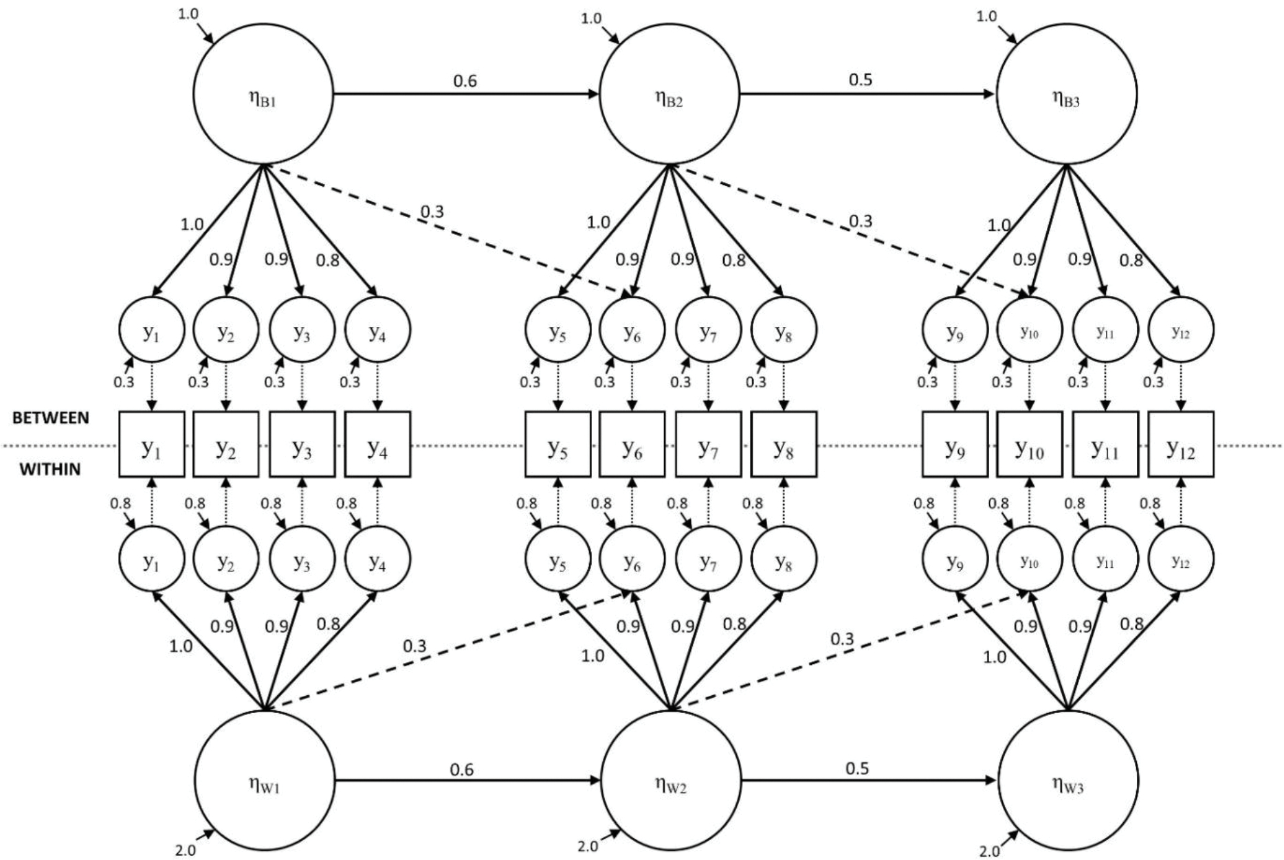
Data generating model. The Misspecified Within model omits the cross loadings (dashed lines) at the within level, and The Misspecified Between omits the cross loadings at the between level model.

We manipulated two primary factors in generating the data: number of clusters and the average cluster size. The number of clusters varied continuously between 30 and 300 (this range covers well above and below the suggested 100 clusters). We varied the average cluster size between 5 and 50. This range captures small to sufficiently large cluster sizes. In practice, smaller clusters might be expected in studies of classrooms and larger clusters could be expected in studies where clustering is based on geography or policy.

Instead of picking specific discrete conditions for cluster size and number of clusters, we allowed these variables to vary continuously between the limits described above. For example, for each replication the value of the number of clusters was sampled from a random discrete uniform condition with lower and upper bounds of 30 and 300, respectively. The same random sampling procedure was used to set the average size of clusters, except that the lower and upper limits were 5 and 50.

To reflect real world applications, cluster sizes were unbalanced within datasets. Real data rarely have balanced clusters except in very controlled study designs. The method proposed in this study does not require the assumption of balanced clusters. Unbalanced data was simulated by fixing the average cluster size but allowing the individual cluster sizes to vary around that average. The degree of unbalance was fixed such that minimum and maximum cluster sizes were 50% smaller or larger than the average cluster size.

With the above specifications, we generated 20,000 independent datasets using the Monte Carlo function of Mplus (Muthén & Muthén, 2017).

Models Specifications

We fit three possible model specifications: the true model, omitted cross loadings at the within level and omitted cross loadings at the between level. They are referred to as the True Model, Misspecified Within, and Misspecified Between, respectively. Fitting three possible model specifications allowed us to investigate performance of all estimators under ideal circumstances as well as circumstances that were more realistic where the model is not correctly specified.

Estimators

For each dataset and model specification, we obtained parameter estimates using three estimators. The first estimator was ML as implemented in Mplus with the “Model = TWOLEVEL” framework. The second estimator was MIIV-2SLS using all possible MIIVs for each equation, denoted by 2SLS-ALLIV. The third estimator was MIIV-2SLS with a subset of MIIVs for each equation such that the equation is overidentified by two degrees of freedom (i.e., $L-K=2$) under the True Model specification. This will be denoted by 2SLS-OVERID2. Both 2SLS-ALLIV and 2SLS-OVERID2 were carried out in R.

Table 1 lists the observed variables and MIIVs for the MIIV-2SLS estimators. The equations listed apply to both levels of the model. To select MIIVs used by 2SLS-OVERID2, we choose the MIIVs that have the highest correlation with the right-hand side variable. We believe this reflects how one would select a subset of MIIVs in practice. For example, if the equation contains one unknown factor loading, we selected MIIVs from the same latent variable plus one additional instrument from the closest latent variable in the causal chain. If the equation contains two unknown factor loadings, we selected two MIIVs from each latent variable.

Table 1.

Observed variables corresponding to MIIV-2SLS equations.

		Instruments
LHS	RHS	ALLIV	OVERID2
		Correctly Specified Models
Factor Loadings
Y2	Y1	Y3, Y4, Y5, Y6, Y7, Y8, Y9, Y10, Y11, Y12	Y3, Y4, Y5
Y3	Y1	Y2, Y4, Y5, Y6, Y7, Y8, Y9, Y10, Y11, Y12	Y2, Y4, Y5
Y4	Y1	Y2, Y3, Y5, Y6, Y7, Y8, Y9, Y10, Y11, Y12	Y2, Y3, Y5
Y6	Y5, Y1	Y2, Y3, Y4, Y7, Y8, Y9, Y10, Y11, Y12	Y2, Y3, Y7, Y8
Y7	Y5	Y1, Y2, Y3, Y4, Y6, Y8, Y9, Y10, Y11, Y12	Y6, Y8, Y10
Y8	Y5	Y1, Y2, Y3, Y4, Y6, Y7, Y9, Y10, Y11, Y12	Y6, Y7, Y10
Y10	Y9, Y5	Y1, Y2, Y3, Y4, Y6, Y7, Y8, Y11, Y12	Y6, Y7, Y11, Y12
Y11	Y9	Y1, Y2, Y3, Y4, Y5, Y6, Y7, Y8, Y10, Y12	Y8, Y10, Y12
Y12	Y9	Y1, Y2, Y3, Y4, Y5, Y6, Y7, Y8, Y10, Y11	Y8, Y10, Y11
LV regressions
Y5	Y1	Y2, Y3, Y4	Y2, Y3, Y4
Y9	Y5	Y1, Y2, Y3, Y4, Y6, Y7, Y8	Y2, Y6, Y7
		Incorrectly Specified Models
Factor Loadings
Y2	Y1	(see correctly specified equations above)
Y3	Y1	(see correctly specified equations above)
Y4	Y1	(see correctly specified equations above)
Y6	Y5	Y1, Y2, Y3, Y4, Y7, Y8, Y9, Y10, Y11, Y12	Y2, Y3, Y7, Y8
Y7	Y5	(see correctly specified equations above)
Y8	Y5	(see correctly specified equations above)
Y10	Y9	Y1, Y2, Y3, Y4, Y5, Y6, Y7, Y8, Y11, Y12	Y6, Y7, Y11, Y12
Y11	Y9	(see correctly specified equations above)
Y12	Y9	(see correctly specified equations above)
LV regressions
Y5	Y1	(see correctly specified equations above)
Y9	Y5	(see correctly specified equations above)

Note: All equations apply to both levels of the model.

As we can see from Table 1, most equations as well the MIIVs remain unchanged when the model is misspecified. According to the robustness properties of MIIV-2SLS (e.g., Bollen et. al., 2018), the equations that remain unchanged will be robust to misspecifications for MIIV-2SLS. For misspecified equations, the MIIV-2SLS estimator is not robust any more. In contrast, the ML estimator is not necessarily robust even for unchanged equations. It is worth mentioning that the set of MIIVs used for 2SLS-ALLIV in the misspecified models uses the set of MIIVs under the True Model specification due to the omitted cross loading. Regarding 2SLS-OVERID2, we use the same set of MIIVs from the True Model specification. Hence, the overidentification degrees of freedom are 3 in misspecified equations.

Simulation Evaluation

The outcome measures that we examined included relative bias, empirical standard deviation of estimates, standard error relative bias, root mean squared error, and proportion of overidentification test rejections given $\alpha =0.05$. Due to space limitation, only selected results will be presented here. More results can be found in the supplementary material. Further, we discretize the average cluster size into three levels (i.e., 5–15, 16–30, 31–50). Since the number of clusters range from 30 to 300, there are 813 difference combinations of number of clusters and cluster size. We also classify the parameters into three types (i.e., Latent Variable Regression, Primary Loading, Cross Loading).

Results

Convergence and Extreme Outliers

Failure to converge can occur for both ML and MIIV-2SLS in this study, though we expected that more models would converge with MIIV-2SLS. If either ML or MIIV-2SLS did not converge, results were thrown out for all three estimators. Overall, less than 0.5% of cases were dropped. Dropping few cases is unlikely to influence the general pattern of results. In cases when ML failed to converge but MIIV-2SLS did converge, the MIIV-2SLS results did appear to be slightly more aberrant than other cases. Though given a small sample it was difficult to draw any serious conclusions from this pattern.

Figure 2 displays a heat map of convergence rates. As expected, MIIV-2SLS had a higher convergence rate, though this difference was small and rates of convergence were generally high for both estimators. In total, 27 models did not converge with MIIV-2SLS, and this was unaffected by model specification. Using ML, 71 models did not converge when the true model was fitted, 80 models did not converge when the within model is misspecified, and 96 models did not converge when the between model is misspecified. It is unsurprising to note that the majority of models that did not converge had both a small number of clusters and a small average cluster size.

Figure 2.

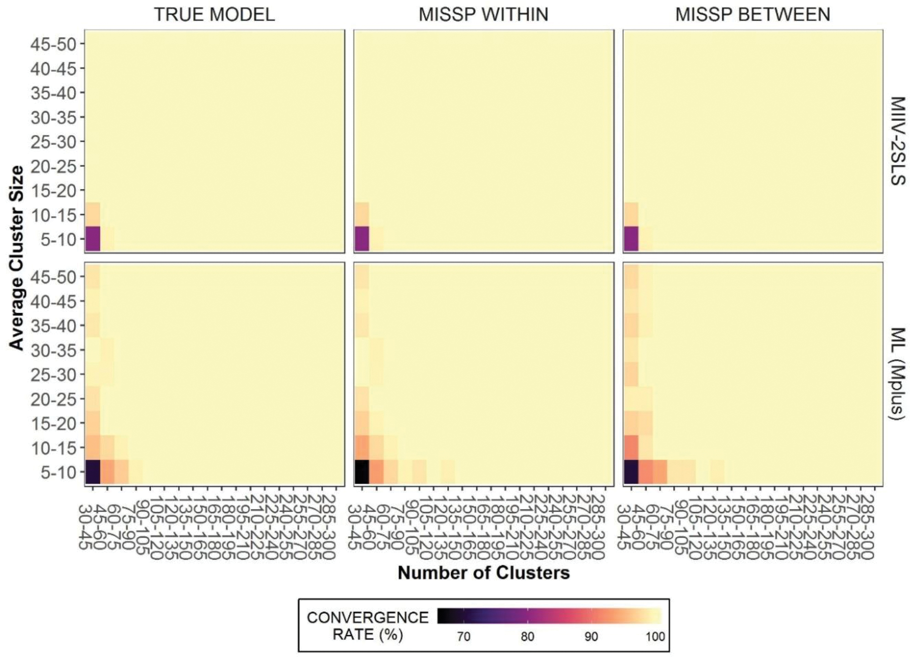
Convergence rate heat map.

Relative Bias

To investigate the accuracy of the estimators, the relative bias of parameter $\mathrm{\theta }$ in each of 813 conditions of number of clusters and cluster size is given by

$$\frac{1}{R}\sum _{r=1}^R\frac{{\widehat{\theta }}_r-\theta }{\theta },$$ (17)

where ${\hat{\theta }}_r$ is the estimate of $\mathrm{\theta }$ for replication $r$ and $R$ is the number of replications in the condition. The average relative bias is then computed by averaging (17) across parameters of the same type.

Figure 3 displays the scatter plot of average relative bias for the True Model specification, as well as the smoothing curves. It is seen that the average relative bias for within level parameters is effectively zero across all conditions and estimators. Regarding the between level parameters, 2SLS-ALLIV tends to be slightly biased when the sample size is small, whereas 2SLS-OVERID2 is less biased than 2SLS-ALLIV. This result is consistent with previous studies that using a smaller set of MIIVs tends to be less biased in small samples whereas this does not matter in larger samples (e.g., Bollen, et al 2007).

Figure 3.

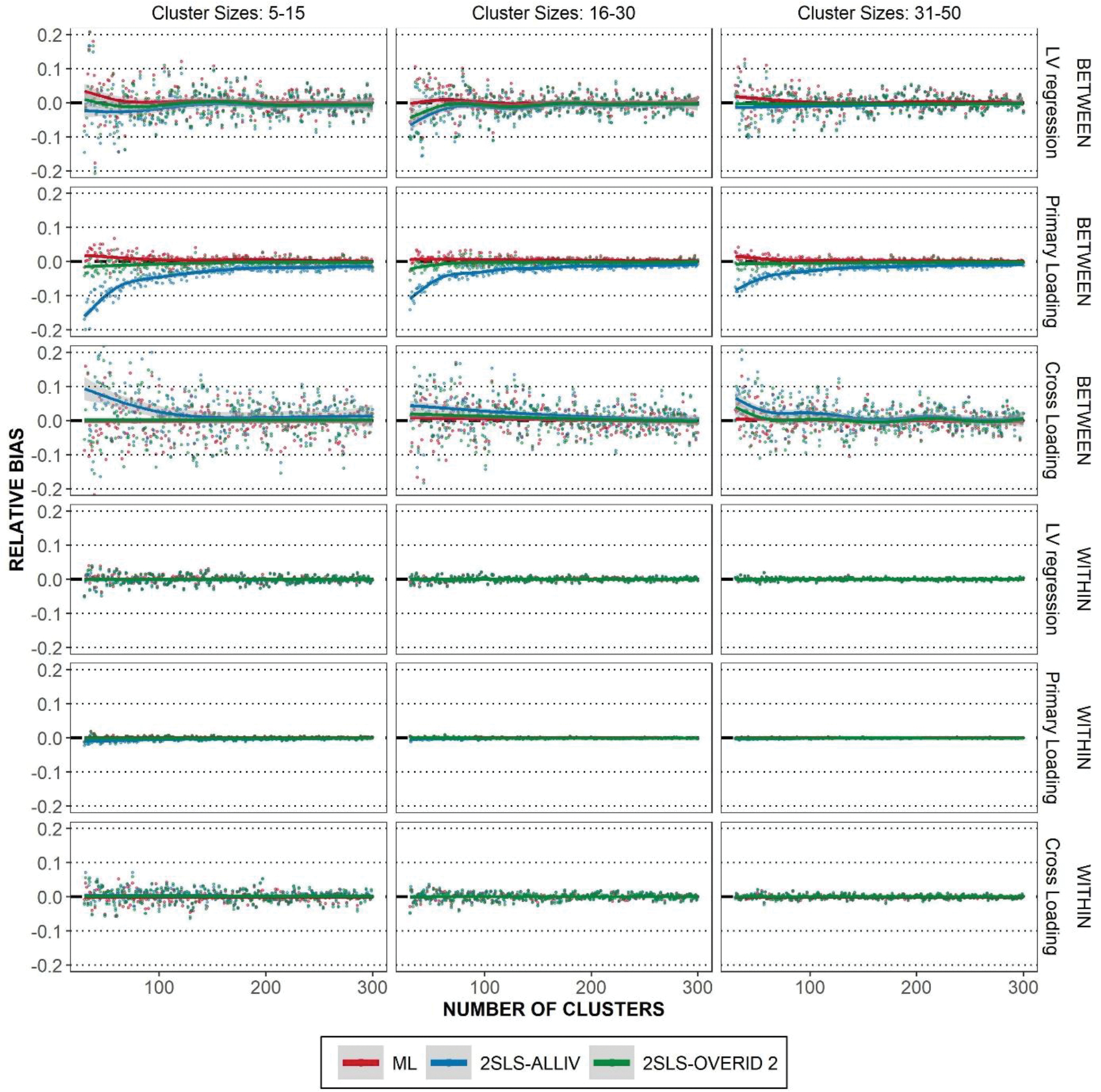
Average relative bias given the true model. Relative bias is averaged and plotted across level of the model, type of parameter, estimator, cluster size and number of clusters. Lowess curve overlaid to show trends.

As shown in Table 1, two equations for factor loadings are misspecified due to omitted factor loadings. The other equations are correctly specified and are expected to be robustly estimated. Figure 4 displays the scatter plot of average relative bias for the Misspecified Within specification. A similar conclusion can be drawn when considering the Misspecified Between specification. Hence, we only focus on the Misspecified Within specification to save space. It is seen that MIIV-2SLS can still consistently estimate the correctly specified equations. The omitted cross loading does not spread the bias to other correctly specified equations in the same level nor the equations in the other level. In contrast, when ML is used, misspecification spreads the bias to some correctly specified equations both in the between level and the within level (Figure 4). It is worth mentioning that the model with a biased ML estimator can fit the data poorly. The replications with poor fits are not excluded when evaluating the bias. Nevertheless, the robustness properties of MIIS-2SLS imply that it can still be reasonable to interpret the estimates in a misspecified model.

Figure 4.

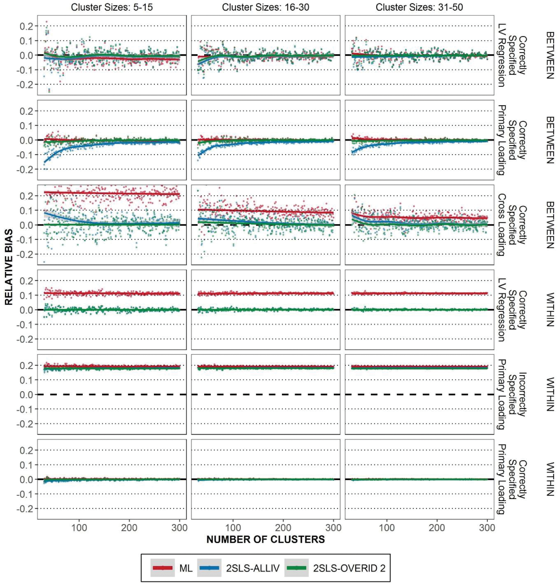
Average relative bias given a misspecified within model. Correct and Incorrect specification is with respect to the MIIV-2SLS equations given in Table 1. Lowess curve overlaid to show trends.

Empirical Standard deviation

As was already mentioned, one possible trade-off when using MIIV-2SLS would be the potential loss of efficiency. To assess the variability of estimates, we use the empirical standard deviation. For any given parameter $\mathrm{\theta }$, the empirical standard deviation of each condition of number of clusters and cluster size is given by

$$s_{\hat{\theta }}=\sqrt{\frac{\sum _{r=1}^R{({\hat{\theta }}_r-\bar{\theta })}^2}{R-1}},$$ (18)

where $R$ is the total number of replications in a condition and $\bar{\theta }$ is the average estimate of $\theta$ in the same condition. Figure 5 illustrates the averaged empirical standard deviations of different parameter types for the True Model specification. Results from the misspecified model conditions are similar and we include them in the supplemental materials. The empirical standard deviations of each estimator are remarkably similar on average. As expected, ML tends to have a slightly lower variability, though this depends on the level of the model and parameter in question. The most notable differences can be seen for parameters with the lowest magnitude (cross loadings). For factor loadings, we see almost no difference between estimators.

Figure 5.

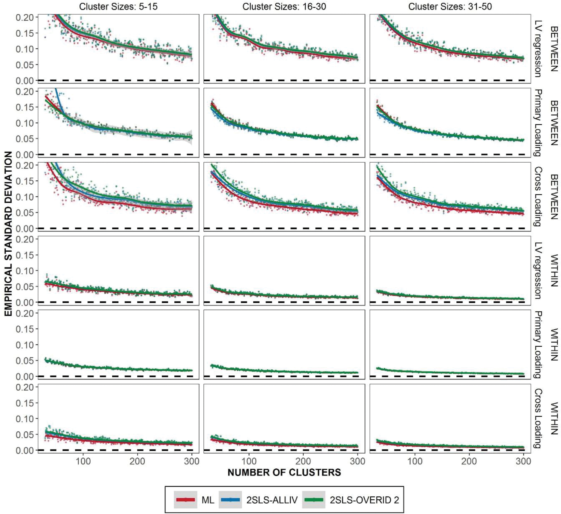
Empirical Standard Deviation of parameter estimates given the true model. Lowess curve overlaid to show trends.

In terms of root mean squared error given by

$$\sqrt{\frac{{\sum }_{r=1}^R{({\widehat{\theta }}_r-\theta )}^2}{R}},$$

it is seen from Figure 6 that ML tends to produce a slightly lower root mean squared error than MIIV-2SLS. However, as the case for empirical standard deviation, the differences between root mean squared errors are generally small. In general, Figures 5 and 6 suggest that ML has a slight efficiency advantage, but MIIV-2SLS does not differ from ML in terms of efficiency in a significant way.

Figure 6.

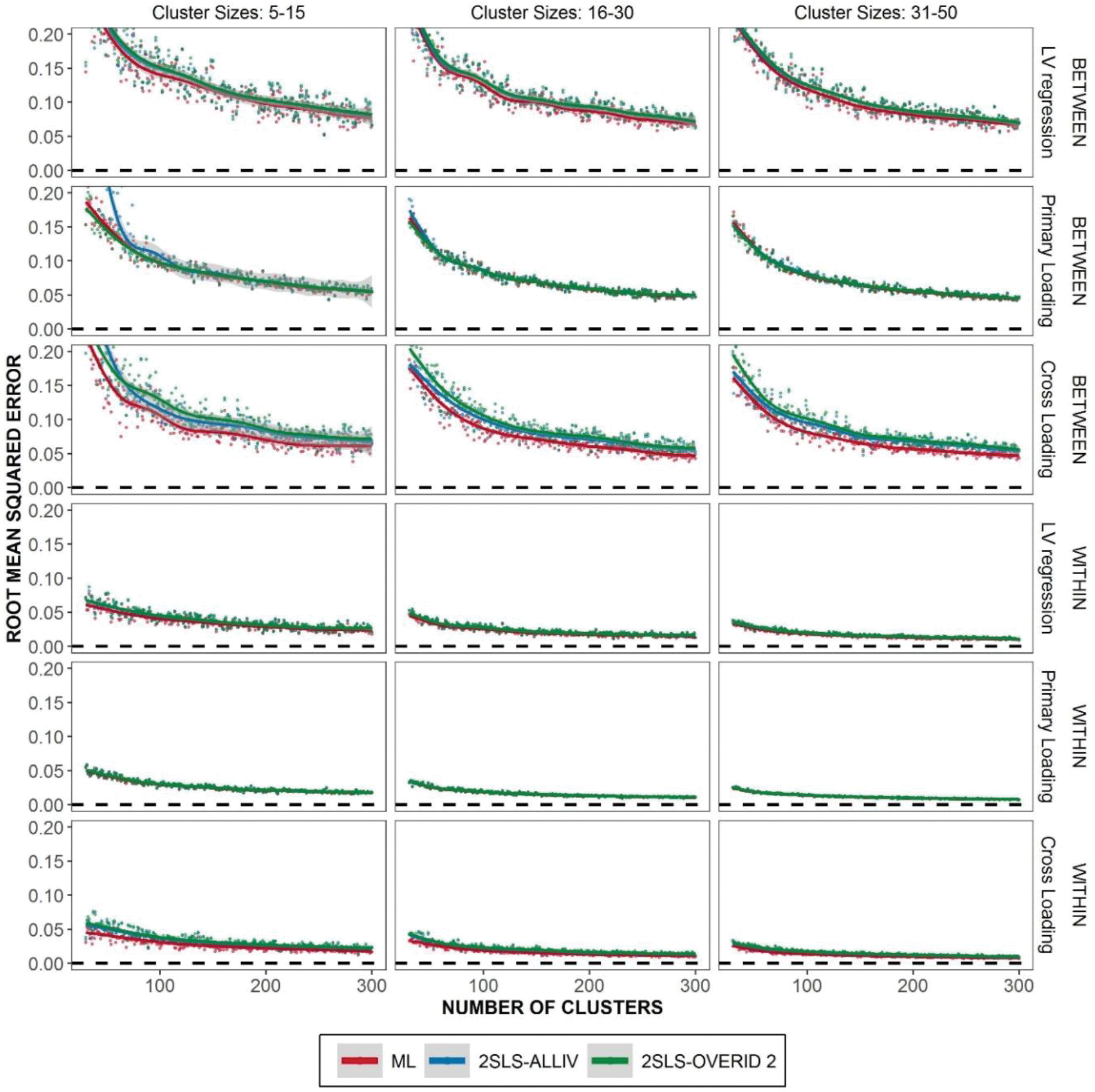
Root Mean Squared Error given true model. Lowess curve overlaid to show trends.

Standard Error Bias

The MIIV-2SLS procedure developed in this study used delta method standard errors. Delta method standard errors are approximate standard errors which are asymptotically unbiased. To verify their performance in finite samples, we consider the standard error bias, computed as the difference between the standard error and the empirical standard deviation, scaled by the empirical standard deviation. The standard error relative bias of a single estimator is given by

$$S{E}_{bias}=\frac{S{E}_r-s_{\hat{\theta }}}{s_{\hat{\theta }}},$$ (19)

where $S{E}_r$ is the standard error for an individual parameter of replication $r$ and $s_{\hat{\theta }}$ is given by Equation (18). The average standard error relative bias is then computed as

$$\frac{1}{R}\sum _{r=1}^R\frac{S{E}_r-s_{\widehat{\theta }}}{s_{\widehat{\theta }}},$$ (20)

where $R$ is the total number of replications in a condition. Figure 6 displays the scatter plot of average standard error relative bias given the True Model specification. Results are similar across all three specifications; we focus on the true model for simplicity and results for other model specifications are included in supplemental materials. Compared to previous simulation outcomes, the values of standard error bias in each condition appear more variable (across all estimators). This is no doubt an artifact of the study design containing a relatively small number of replications per condition. The smoothed averages reflect what we would expect given larger cell sizes.

On average, there was little standard error bias, across all three estimators. When there was bias, it tended to be positive bias on average, suggesting the standard errors are more likely to be conservative (i.e., too large). These results suggest that the delta method standard errors used with MIIV-2SLS, are generally adequate for capturing the true variability across a range of sample sizes and parameters, except in the smallest sample size conditions which we discuss next.

In the smallest sample size conditions (small average cluster size and small number of clusters) for between level factor loadings, the standard error bias for 2SLS-ALLIV appears rather high and positive. This result was extreme and unexpected. It is partly a result of several extreme standard error outliers; sensitivity analyses (removing some outliers) reduced the magnitude of this effect, but overall bias remained pronounced for these parameters given the smallest sample sizes. This result might suggest that these delta method standard errors are unstable in very small samples, when using a large number of instruments. Similar to the relative bias results, this problem was fully mitigated by using a subset of instruments (2SLS-OVERID2).

95% Confidence Intervals

The standard errors are often used to construct confidence intervals. We would expect the 95% confidence intervals to cover the true population value 95% of the time. Only the True Model specification is considered here since the confidence interval is not so meaningful in a misspecified equation. It is seen from Figure 8 that the average coverage probability is generally close to the nominal level (i.e., 95%), especially when the number of clusters is large.

Figure 8.

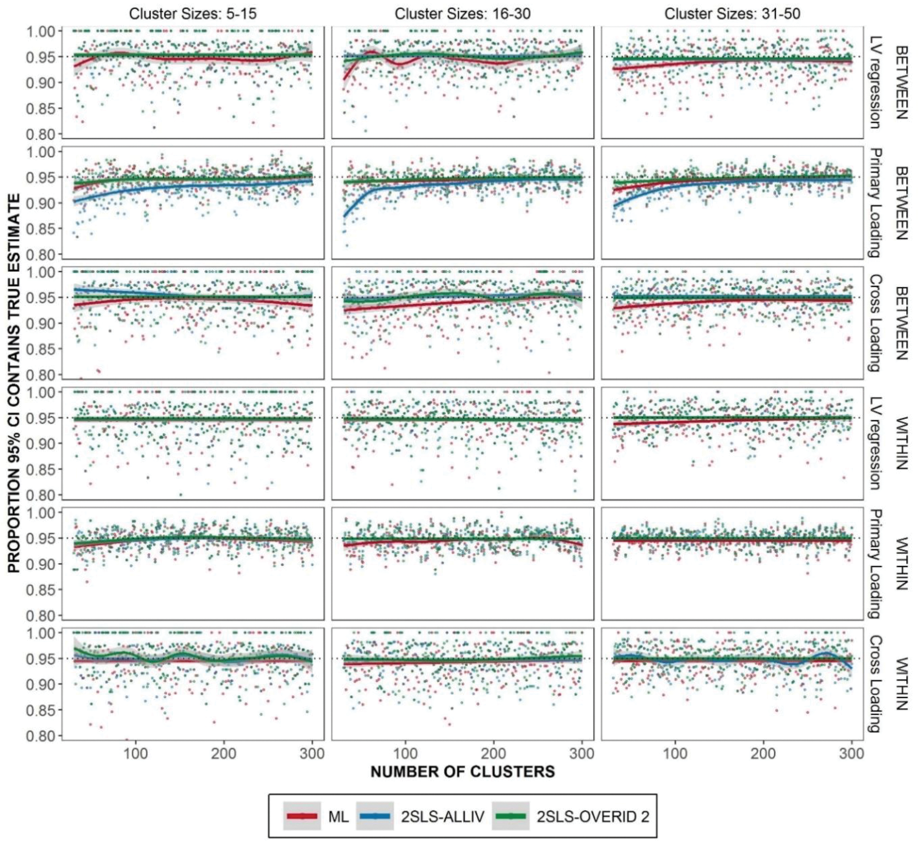
Proportion of 95% confidence intervals which contain the population parameter given the true model. Lowess curve overlaid to show trends.

Multilevel Overidentification Test for Equations

Finally, we examined the performance of the proposed multilevel overidentification equation test. Rejecting the null hypothesis suggests that one or more MIIVs correlate with the equation’s error term. In the correctly specified models, we would expect the overidentification test to reject the null hypothesis at the level of alpha $(\alpha =.05)$. Given misspecifications, we expected the test to reject the null hypothesis at a higher rate. Each overidentified equation has a test statistic and given the number of equations, this creates a multiple testing problem. To take account of this, we estimated rejection rates based on the unadjusted p-values and the Benjamini-Hochberg (B-H) corrected p-values to control for the false discovery rate (Benjamini and Hochberg, 1995). Benjamini-Hochberg correction was applied independently at each replication and level of the model.

Given the True Model specification¹, the multilevel overidentification test rejected the null hypothesis at or below the level of alpha. There are not any appreciable differences between the 2SLS-ALLIV and 2SLS-OVERID2 estimators. When using the unadjusted p-values the rejection rate is generally much closer to 0.05. Using the B-H corrected standard errors leads to effectively 0% rejection rates. Given that the unadjusted p-values do not lead to rejection rates higher than 0.05, this suggests that correcting for multiple testing may not be completely necessary.

Figures 9 and 10 illustrate the empirical rejection proportion of misspecified equations in the misspecified within model and the misspecified between model, respectively. Correctly specified equations in these conditions are unchanged from the True Model specification. Hence, they are not repeated here. For misspecified equations at the within level (Figure 7) the multilevel overidentification test rejects the null hypothesis almost 100% of the time, except in very small numbers of clusters where the lowest rate of rejecting the null is still around 0.8. There are small differences in the B-H rejection rates leading to slightly lower power in small samples. For misspecified equations at the between level (Figure 8) the Sargan test has less power especially given smaller sample sizes. 2SLS-OVERID2 rejects the null hypothesis at a much higher rate as well, which suggests that the effectiveness of multilevel test depends on the MIIVs used. Given medium to large cluster sizes, both 2SLS-ALLIV and 2SLS-OVERID2 reach roughly 80% power when number of clusters reaches 200–250 clusters, using the unadjusted p-values. The difference in the B-H p-values are starker in this example, such that using adjusted p-values leads to a dramatic loss in power.

Figure 9.

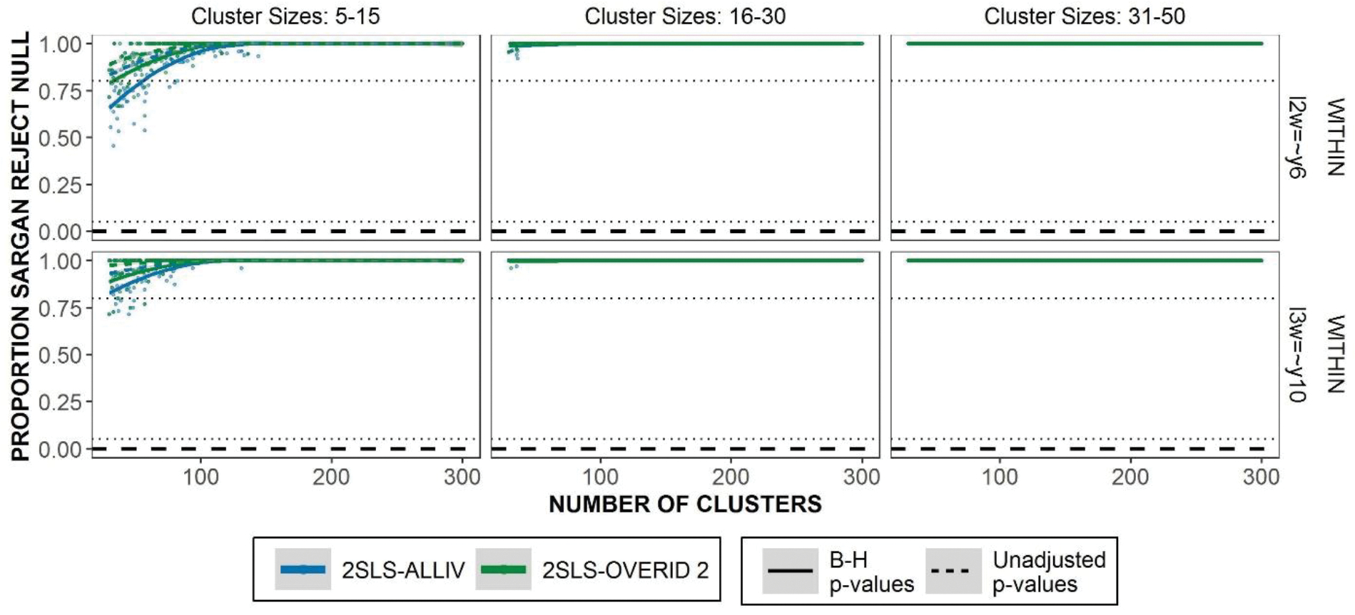
Proportion of Multilevel Overidentification Test rejecting the null hypothesis for misspecified equations in the misspecified within model. Dotted line marks 80% rejection rate.

Figure 10.

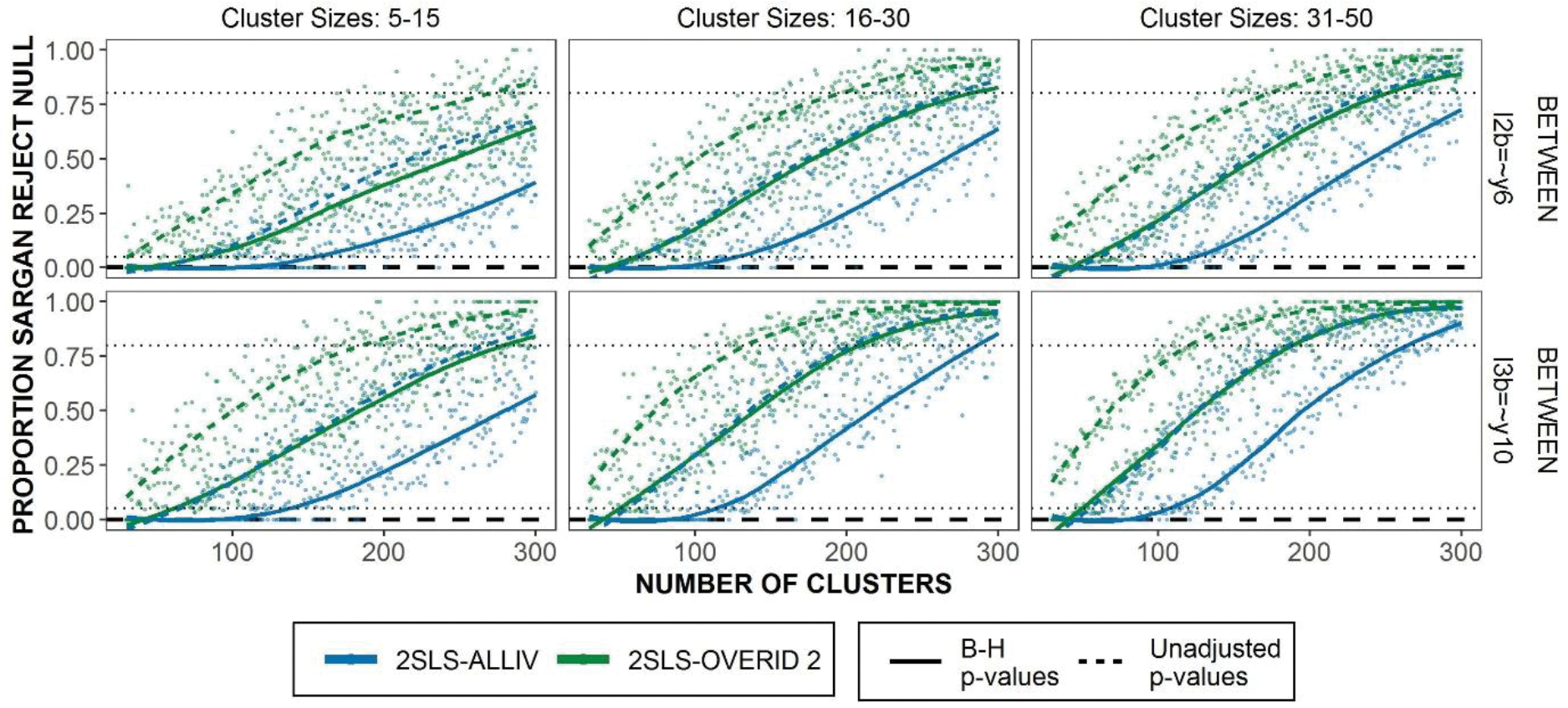
Proportion of Multilevel Overidentification Test rejecting the null hypothesis for misspecified equations in the misspecified between model. Dotted line marks 80% rejection rate. Lowess curve overlaid to show trends.

Figure 7.

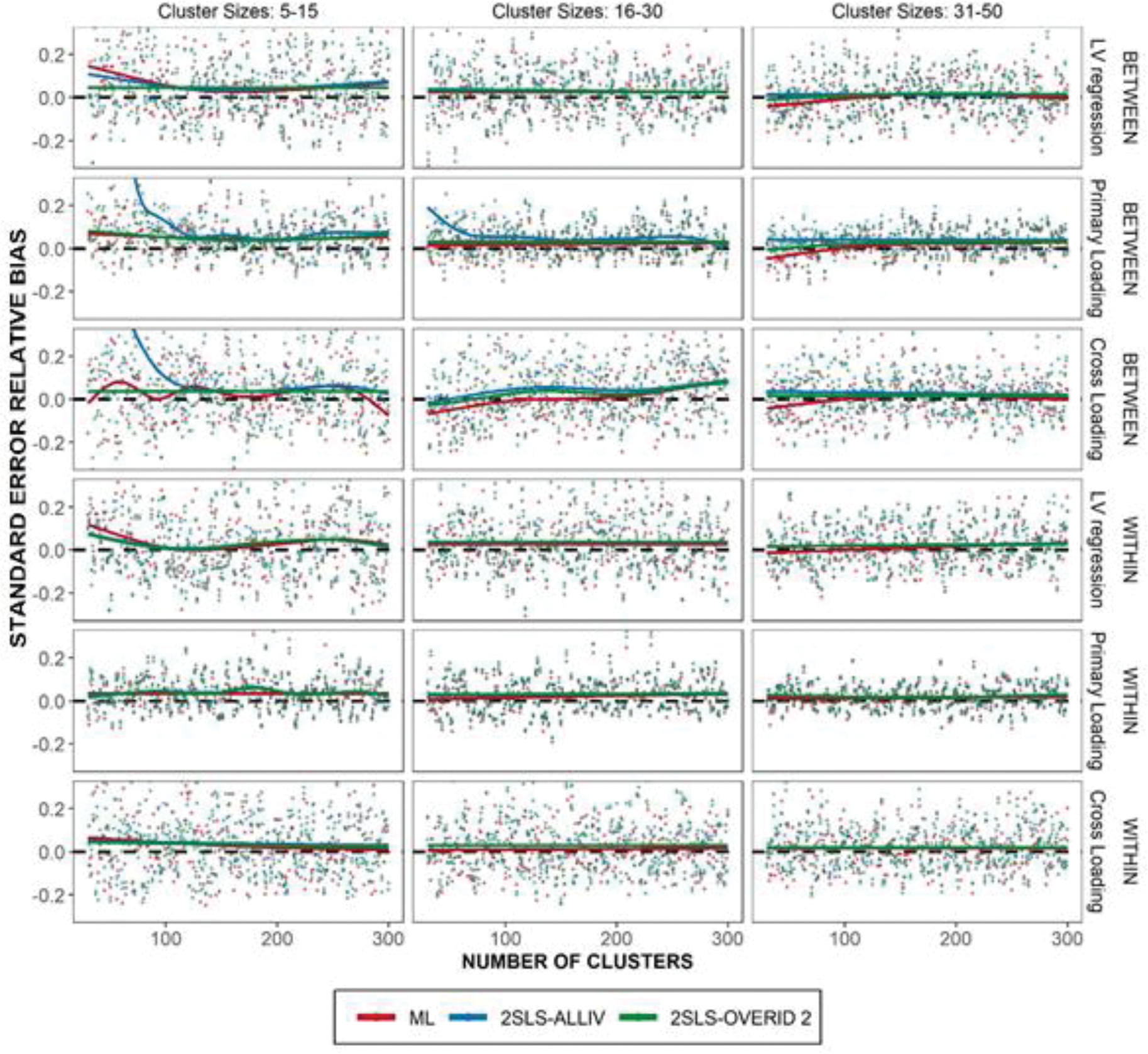
Standard Error Relative Bias given true model. Lowess curve overlaid to show trends.

Discussion

This study examined several research questions about the properties of MIIV-2SLS in finite samples. Our research questions focused on robustness, efficiency, standard errors, sample size, and model tests. We review our results with respect to each of these.

(1). Robustness.

This study demonstrated that MIIV-2SLS for MSEMs retains the expected robustness to the spread of model misspecification. This quality may be especially important for MSEMs where model misspecification can spread bias both within level as well as between levels when using system-wide estimators. In line with the suggestion in Yuan and Bentler (2007), this study demonstrated that bias can spread across levels when using ML.

(2). Efficiency.

We examine the relative efficiency of the ML and the MIIV-2SLS estimators of MSEMs. Any difference in efficiency using MIIV-2SLS was slight in our simulation. One could easily argue that the additional robustness qualities is a valuable tradeoff for a very slight loss in efficiency. This is especially true if one believes that all models are approximations.

(3). Standard errors.

The delta method standard errors as applied in this study were generally adequate to capture sampling variability in finite samples. The one exception to this was in the smallest sample sizes when using 2SLS-ALLIV (all possible MIIVs). Given those conditions, our results showed that standard errors could be unstable and were magnitudes larger than expected. Importantly, given the smallest sample sizes tested in this study, simply using 2SLS-OVERID2 (a subset of possible MIIVs) fixed any instability in standard errors.

(4). Sample Size.

Our results suggest that MIIV-2SLS is a promising alternative to ML when there are fewer than 100 clusters. MIIV-2SLS performed well in sample sizes well below 100 clusters—the suggested minimum for ML. Being able to estimate models with fewer than 100 clusters is likely to be very valuable for researchers. In samples with fewer than 50 clusters, our results indicated that one should use a subset of MIIVs. We tested a rather extreme minimum of 30 clusters in this study; we are hesitant to suggest one could perform MIIV-2SLS consistently in samples this small. The combination of few clusters and small number of clusters had one rather serious side effect of positive biased standard errors when using all instruments (2SLS-ALLIV). Based on this simulation, we would suggest that between 50 and 100 clusters are acceptable for using MIIV-2SLS. At the same time, in these simulations ML also performed reasonably well across the same range of sample sizes. This performance could be partially an artifact of generally well-behaved data. One is likely to encounter more problems in small samples with real data.

(5). Model Fit.

The multilevel overidentification test we presented had appropriate rejection rates given correctly specified equations, high power to detect misspecification at the within level model, and variable power to detect misspecifications at the between level model. At the between level model, one would need greater than 100 clusters to detect the misspecifications in this study.

One might be tempted to compare the ability of the multilevel overidentification test to detect misspecification at the between level model with some of the ML based alternatives (e.g., Yuan & Bentler, 2007; Ryu & West, 2014). However, our study contained a rather minor misspecification while other studies of ML model fit have assessed major misspecifications (two factor model being fit as a single factor). To directly compare our multilevel test to other ML based model fit techniques we would need to assess the multilevel test in a more comparable simulation study.

Limitations & Future Directions

One of the primary limitations of any simulation study is generalizability to other models and conditions. In this study, we examined one model across a range of conditions. One might reasonably assume that the conclusions from this study could extend to a broader set of models. At the same time, it is imperative to realize that these results do not capture all the possible complexities in MSEMs, and we cannot fully predict how these results will reflect on a completely different model. In this way, more research is necessary to understand other model complexities. Meanwhile, various Bayesian methods have been used to estimate MSEM model (e.g., Depaoli & Clifton, 2015; Holtmann et. al., 2016). Since the Bayesian methods often rely on the entire model specification, we conjecture that MIIV-2SLS will be more robust against structural misspecifications. It will be of interest to conduct a thorough simulation study to compare the performance of Bayesian methods and the proposed MIIV-2SLS approach, especially in small samples.

One particularly salient example of this problem with MIIV-2SLS has to do with the availability and selection MIIVs. We only examined overidentified models where every equation had many possible MIIVs. It is possible to encounter models with many fewer instruments. In these models, some equations may be underidentified or perhaps only exactly identified for MIIV-2SLS (meaning no overidentification test). In other applications, there may be plenty of MIIVs but the instruments could be weak. We did not examine these scenarios and future research is needed to study different types of models with varying qualities and quantities of MIIVs.

There are technical limitations about the types of models that can be handled with MIIV-2SLS in MSEMs, as it currently stands. Our current MSEM estimator does not handle categorical data, random slopes, or more than two levels. Additionally, this study entirely focused on estimating coefficients and did not consider the mean structure of the model as in Fisher and Bollen (2020). We leave it as a topic of future inquiry. Further, it is often of interest to estimate the covariance parameters (e.g., residual and latent variable variances) in multi-level modeling. As mentioned in Introduction, system-wide estimators are often used to estimate those parameters. Consequently, they are not robust against structural misspecifications.

Conclusion

To our knowledge, the current study is the first to demonstrate estimating random intercept MSEMs with MIIV-2SLS. The primary goal of this research was to adapt MIIV-2SLS estimation for MSEMs and study the empirical performance. The MIIV-2SLS for MSEM is robust across levels in that misspecification errors at one level (e.g., between level) do not impact estimates at the other level (e.g., within level). Furthermore, Bollen’s (2020) and Bollen, Gates, and Fisher’s (2018) robustness conditions for MIIV-2SLS in single level models carry over to each level in MSEM. This means we can use these analytic conditions to know which type of misspecifications affect an equation and which do not. Moreover, ours is the first to propose a multilevel overidentification test for equations.

Overall, our results suggest that MIIV-2SLS is a reasonable alternative or supplement to ML given random intercept MSEMs. Of course, the MIIV-2SLS procedure developed in this study is not intended to replace ML. Instead, our hope is to add MIIV-2SLS an additional tool for MSEM estimation.

References

- Bentler Peter M., & Liang, J. (2003). Two-level mean and covariance structures: Maximum likelihood via an EM algorithm. In Reise SP & Duan N (Eds.), Multilevel Modeling: Methodological Advances, Issues, and Applications. (pp. 53–70). Mahwah, N.J: Lawrence Erlbaum Associates. [Google Scholar]
- Bollen KA (1989). Structural Equations with Latent Variables. New York: Wiley-Interscience. [Google Scholar]
- Bollen KA (1996). An alternative two stage least squares (2SLS) estimator for latent variable equations. Psychometrika, 61(1), 109–121. [Google Scholar]
- Bollen KA (2019). Model Implied Instrumental Variables (MIIVs): An Alternative Orientation to Structural Equation Modeling. Multivariate Behavioral Research, 54(1), 31–46. [DOI] [PMC free article] [PubMed] [Google Scholar]
- Bollen KA (2020). When Good Loadings Go Bad: Robustness in Factor Analysis. Structural Equation Modeling: A Multidisciplinary Journal, 27 (4), 515–524. [DOI] [PMC free article] [PubMed] [Google Scholar]
- Bollen KA, Gates KM, & Fisher Z (2018). Robustness Conditions for MIIV-2SLS When the Latent Variable or Measurement Model is Structurally Misspecified. Structural Equation Modeling: A Multidisciplinary Journal, 25(6), 848–859. [DOI] [PMC free article] [PubMed] [Google Scholar]
- Bollen KA, Kirby JB, Curran PJ, Paxton PM, & Chen F (2007). Latent Variable Models Under Misspecification: Two-Stage Least Squares (2SLS) and Maximum Likelihood (ML) Estimators. Sociological Methods & Research, 36(1), 48–86. [Google Scholar]
- Bollen KA, Kolenikov S, & Bauldry S (2014). Model-implied instrumental variable-generalized method of moments (MIIV-GMM) estimators for latent variable models. Psychometrika, 79(1), 20–50. [DOI] [PMC free article] [PubMed] [Google Scholar]
- Bollen KA, & Maydeu-Olivares A (2007). A polychoric instrumental variable (PIV) estimator for structural equation models with categorical variables. Psychometrika, 72(3), 309–326 [Google Scholar]
- Browne MW (1984). Asymptotically distribution free methods for the analysis of covariance structures. British Journal of Mathematical and Statistical Psychology, 37(1), 62–83. [DOI] [PubMed] [Google Scholar]
- Depaoli S, & Clifton JP (2015). A Bayesian approach to multilevel structural equation modeling with continuous and dichotomous outcomes. Structural Equation Modeling: A Multidisciplinary Journal, 22(3), 327–351. [Google Scholar]
- Fisher ZF, & Bollen KA (2020). An instrumental variable estimator for mixed indicators: Analytic derivatives and alternative parametrizations. Psychometrika, 85(3), 660–683. [DOI] [PMC free article] [PubMed] [Google Scholar]
- Fisher ZF, Bollen KA, & Gates KM (2019). A limited information estimator for dynamic factor models. Multivariate Behavioral Research, 54(2), 246–263. [DOI] [PMC free article] [PubMed] [Google Scholar]
- Fisher Z, Bollen K, Gates K, & Rönkkö M (2017). Model Implied Instrumental Variable (MIIV) Estimation of Structural Equation Models. R package version 0.5.3. [Google Scholar]
- Fox J (1979). Simultaneous Equation Models and Two-Stage Least Squares. Sociological Methodology, 10, 130. [Google Scholar]
- Gates KM, Fisher ZF, & Bollen KA (2020). Latent variable GIMME using model implied instrumental variables (MIIVs). Psychological Methods, 25(2), 227–242 [DOI] [PMC free article] [PubMed] [Google Scholar]
- Holtmann J, Koch T, Lochner K, & Eid M (2016). A Comparison of ML, WLSMV, and Bayesian Methods for Multilevel Structural Equation Models in Small Samples: A Simulation Study. Multivariate Behavioral Research, 51(5), 661–680. [DOI] [PubMed] [Google Scholar]
- Hox JJ, & Maas C (2004). Multilevel structural equation models: The limited information approach and the multivariate multilevel approach. In van Montford K, Oud J, & Satorra A (Eds.), Recent Developments on Structural Equation Models (pp. 135–149). Dordrecht, Netherlands: Kluwer Academic Publishers. [Google Scholar]
- Hsu H-Y, Kwok O, Lin JH, & Acosta S (2015). Detecting Misspecified Multilevel Structural Equation Models with Common Fit Indices: A Monte Carlo Study. Multivariate Behavioral Research, 50(2), 197–215. [DOI] [PubMed] [Google Scholar]
- Jin S, & Cao C (2018). Selecting polychoric instrumental variables in confirmatory factor analysis: An alternative specification test and effects of instrumental variables. British Journal of Mathematical and Statistical Psychology, 71(2), 387–413. [DOI] [PubMed] [Google Scholar]
- Jin S, Yang-Wallentin F, Bollen KA. (2021). A unified model-implied instrumental variable approach for structural equation modeling with mixed variables. Psychometrika, 86(2), 564–594. [DOI] [PMC free article] [PubMed] [Google Scholar]
- Julian M (2001). The Consequences of Ignoring Multilevel Data Structures in Nonhierarchical Covariance Modeling. Structural Equation Modeling: A Multidisciplinary Journal, 8(3), 325–352. [Google Scholar]
- Liang J, & Bentler PM (2004). An EM algorithm for fitting two-level structural equation models. Psychometrika, 69(1), 101–122. [Google Scholar]
- Muthén LK and Muthén BO (2017). Mplus User’s Guide. Eighth Edition. Los Angeles, CA: Muthén & Muthén. [Google Scholar]
- Neale MC, Hunter MD, Pritikin JN, Zahery M, Brick TR, Kirkpatrick RM, Estabrook R, Bates TC, Maes HH, Boker SM (2016). “OpenMx 2.0: Extended structural equation and statistical modeling.” Psychometrika, 81(2), 535–549. [DOI] [PMC free article] [PubMed] [Google Scholar]
- Nestler S (2014). How the 2SLS/IV estimator can handle equality constraints in structural equation models: A system-of-equations approach. British Journal of Mathematical and Statistical Psychology, 67(2), 353–369. [DOI] [PubMed] [Google Scholar]
- Nestler S (2015a). A specification error test that uses instrumental variables to detect latent quadratic and latent interaction effects. Structural Equation Modeling: A Multidisciplinary Journal, 22(4), 542–551. [Google Scholar]
- Nestler S (2015b). Using instrumental variables to estimate the parameters in unconditional and conditional second-order latent growth models. Structural Equation Modeling: A Multidisciplinary Journal, 22(3), 461–473. [Google Scholar]
- Rosseel Y (2012). lavaan: An R Package for Structural Equation Modeling. Journal of Statistical Software, 48(2), 1–36. [Google Scholar]
- Ryu E (2014). Model fit evaluation in multilevel structural equation models. Frontiers in Psychology, 5(81) 1–9. [DOI] [PMC free article] [PubMed] [Google Scholar]
- Ryu E, & West SG (2009). Level-Specific Evaluation of Model Fit in Multilevel Structural Equation Modeling. Structural Equation Modeling: A Multidisciplinary Journal, 16(4), 583–601. [Google Scholar]
- Sargan JD (1958). The estimation of economic relationships using instrumental variables. Econometrica: Journal of the Econometric Society, 393–415. [Google Scholar]
- Searle SR, Casella G, & McCulloch CE (1992). Variance components. New York: Wiley. [Google Scholar]
- Wang Y & Kim ES (2017) Evaluating Model Fit and Structural Coefficient Bias: A Bayesian Approach to Multilevel Bifactor Model Misspecification. Structural Equation Modeling: A Multidisciplinary Journal, 24(5), 699–713,. [Google Scholar]
- Yuan K-H, & Bentler PM (2007). Multilevel Covariance Structure Analysis by Fitting Multiple Single-Level Models. Sociological Methodology, 37(1), 53–82. [DOI] [PMC free article] [PubMed] [Google Scholar]
Associated Data
This section collects any data citations, data availability statements, or supplementary materials included in this article.