A COMPOSITIONAL MODEL TO ASSESS EXPRESSION CHANGES FROM SINGLE-CELL RNA-SEQ DATA

Abstract

On the problem of scoring genes for evidence of changes in the distribution of single-cell expression, we introduce an empirical Bayesian mixture approach and evaluate its operating characteristics in a range of numerical experiments. The proposed approach leverages cell-subtype structure revealed in cluster analysis in order to boost gene-level information on expression changes. Cell clustering informs gene-level analysis through a specially-constructed prior distribution over pairs of multinomial probability vectors; this prior meshes with available model-based tools that score patterns of differential expression over multiple subtypes. We derive an explicit formula for the posterior probability that a gene has the same distribution in two cellular conditions, allowing for a gene-specific mixture over subtypes in each condition. Advantage is gained by the compositional structure of the model not only in which a host of gene-specific mixture components are allowed but also in which the mixing proportions are constrained at the whole cell level. This structure leads to a novel form of information sharing through which the cell-clustering results support gene-level scoring of differential distribution. The result, according to our numerical experiments, is improved sensitivity compared to several standard approaches for detecting distributional expression changes.

1. Introduction.

The ability to measure genome-wide gene expression at single-cell resolution has accelerated the pace of biological discovery. Overcoming data analysis challenges caused by the scale and unique variation properties of single-cell data will surely fuel further advances in immunology (Papalexi and Satija (2017)), developmental biology (Marioni and Arendt (2017)), cancer (Navin (2015)) and other areas (Nawy (2013)). Computational tools and statistical methodologies created for data of lower resolution (e.g., bulk RNA-seq) or lower dimension (e.g., flow cytometry) guide our response to the data-science demands of new measurement platforms, but they remain inadequate for efficient knowledge discovery in this rapidly advancing domain (Bacher and Kendziorski (2016)).

An important feature of single-cell studies that could be leveraged better statistically is the fact that cells populate distinct, identifiable subtypes determined by lineage history, epigenetic state, the activity of various transcriptional programs or other distinguishing factors. Extensive research on clustering cells has produced tools for identifying subtypes, including SC3 (Kiselev et al. (2017)), CIDR (Lin, Troup and Ho (2017)) and ZIFA (Pierson and Yau (2015)). We hypothesize that such subtype information may be usefully utilized in other inference procedures in order to improve their operating characteristics.

Assessing the magnitude and statistical significance of changes in gene expression associated with changes in cellular condition has been a central statistical problem in genomics. New tools specific to the single-cell RNA-seq data structure, including MAST (Finak et al. (2015)), scDD (Korthauer et al. (2016)), and D3E (Delmans and Hemberg (2016)) have been deployed to address this problem. These tools respond to scRNA-seq characteristics, such as high prevalence of zero counts and gene-level multimodality, but they do not fully exploit cellular-subtype information and, therefore, may be underpowered in some settings. The proposed method, which uses negative binomial mixtures to measure changes in a gene’s marginal sampling distribution, acquires sensitivity to a variety of distributional effects by how it integrates gene-level data with subtype information. From input data the associated R package scDDboost¹ prioritizes genes with a local false-discovery rate against the null hypothesis of no condition effect on the marginal sampling distribution. The complement of this rate is an empirical Bayesian posterior probability of differential distribution (DD). By incorporating transciptomic information on cell subtypes, scDDboost leverages useful and previously untapped information on each gene’s expression sampling distribution.

Through the compositional model underlying scDDboost, subtypes inferred by clustering inform the analysis of gene-level expression. The proposed methodology merges two lines of computation after cell clustering: one concerns patterns of differential expression among the cellular subtypes, and here we take advantage of the powerful EBseq method for detecting patterns in negative-binomially-distributed expression data (Leng et al. (2013)). The second concerns the counts of cells in various subtypes; for this we propose a double Dirichlet mixture distribution to model the pair of multinomial probability vectors for subtype counts in two experimental conditions. Further elements are developed on the selection of the number of subtypes and on accounting for uncertainty in the cluster output, in order to provide an end-to-end solution to the differential distribution problem. We note that modularity in the necessary elements provides some methodological advantages. For example, improvements in clustering may be used in place of the default clustering without altering the form of downstream analysis. Also, by avoiding Markov chain Monte Carlo, scDDboost computations are relatively inexpensive for a Bayesian procedure.

To set the context by way of example, Figure 1 highlights the ability of scDDboost to sense subtype composition changes and thus detect subtle gene expression changes between conditions. The three panels on the left compare expression from 91 human stem cells known to be in the G1 phase of the cell cycle, as well as from 76 such cells known to be in the G2/M phase (Leng et al. (2015)) in three genes (BIRC5, HMMR and CKAP2), which we happen to know from prior studies have differential activity between G1 and G2/M (Li and Altieri (1999), Sohr and Engeland (2008), Dominguez et al. (2016)). Several standard statistical tools applied to the data behind Figure 1 do not find the observed differences in any of these genes to be statistically significant when controlling the false discovery rate (FDR) at 5%, but scDDboost does include these genes on its 5% FDR list. Considering prior studies, these subtle distributional changes are probably not false discoveries. The right panel in Figure 1 shows these three among many other genes also known to be involved in cell-cycle regulation but not identified by standard tools as altered between G1 and G2/M at the 5% FDR level. The color panel provides insight into why scDDboost has identified these genes. For this data set, six cellular subtypes were identified in the first step of scDDboost (colors red, blue, green and orange are visible). These subtypes have changed in their proportions between G1 and G2/M; there is a lower proportion of red cells and a greater proportion of orange cells in G2/M, for example. These proportion shifts, which are inferred from genome-wide data, stabilize gene-specific statistics that measure changes between conditions in the mixture distribution of expression and, thereby, increase power. We note that scDDboost agrees with other statistical tools on very strong differential-distribution signals (not shown), but it has the potential to increase power for subtle signals owing to its unique approach to leveraging cell subtype information.

Fig. 1.

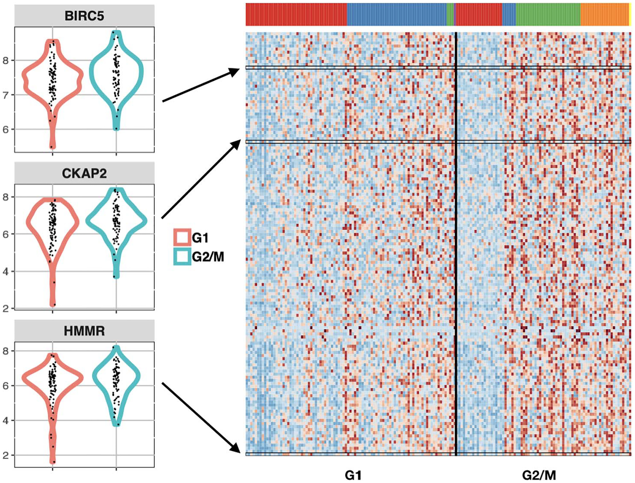
Genes involved in cell cycle that are identified by scDDboost, but not standard approaches, as differentially distributed between cell-cycle phases G1 and G2/M in human embryonic stem cells (GSE64016). Density estimates on the left show expression data (log2 scale) of three genes identified by scDDboost at 5% FDR but not similarly identified by MAST, scDD or DESeq2. Prior studies have shown that the expression of BIRC5, CKAP2 and HMMR is dependent on the phase of cell cycle, suggesting that these subtle shifts are not false positives. Heatmap (right) shows these three genes among 137 other cell-cycle genes (GO:0007049) identified exclusively by scDDboost, with expression from low (blue) to high (red). Cells (columns) are clustered by their genome-wide expression profiles into distinct cellular subtypes, as indicated by the color panel.

Numerical experiments on both synthetic and published scRNA-seq data bear out the incidental finding in Figure 1 that scDDboost has sensitivity for detecting subtle distribution changes. In these experiments we take advantage of splatter for generating synthetic data (Zappia, Phipson and Oshlack (2017)) as well as the compendium of scRNA-seq data available through conquer (Soneson and Robinson (2018)). Additional numerical experiments show a relationship between scDDboost findings and more mechanistic attempts to parameterize transcriptional activation (Delmans and Hemberg (2016)). Finally, we establish first-order asymptotic results for the methodology.

On manuscript organization we present the modeling and methodology elements in Section 2, numerical experiments in Section 3, asymptotic analysis in Section 4 and a discussion in Section 5. We relegate some details to an Appendix and many others to the Supplementary Material (Ma et al. (2021)).

2. Modeling.

2.1. Data structure, sampling model and parameters.

In modeling scRNA-seq data we imagine that each cell $c$ falls into one of $K>1$ classes, which we think of as subtypes or subpopulations of cells. For notation, $z_c=k$ means that cell $c$ is of subtype $k$, with the vector $z=\left(z_c\right)$ recording the states of all sampled cells. Knowledge of this class structure prior to measurement is not required, as it will be inferred as necessary from available genomic data. We expect that cells arise from multiple experimental conditions, such as by treatment-control status or some other factors measured at the cell level, but we present our development for the special case of two conditions. Notationally, $y=\left(y_c\right)$ records the experimental condition, say $y_c=1$ or $y_c=2$. Let’s say condition $j$ measures $n_j={\sum }_{c}1\left[y_c=j\right]$ cells, and, in total, we have $n=n_1+n_2$ cells in the analysis. The examples in Section 3 involve hundreds to thousands of cells. Further, let

$$t_k^j=t_k^j\left(y,z\right)=\sum _{c}1\left[y_c=j,z_c=k\right]$$ (1)

denote the number of cells of subtype $k$ in condition $j$, and $X_{g,c}$ denote the normalized expression of gene $g$ in cell $c$. This is one entry in a typically large genes-by-cells data matrix $X$. Thus, the data structure entails an expression matrix $X$, a treatment label vector $y$ and a vector $z$ of latent subtype labels.

We treat subtype counts in the two conditions, $t^1=\left(t_1^1,t_2^1,\dots ,t_K^1\right)$ and $t^2=(t_1^2,t_2^2,\dots ,t_K^2$), as independent multinomial vectors, reflecting the experimental design. Explicitly,

$$t^1\mid y~{\text{Multinomial}}_K\left(n_1,\varphi \right)\text{ and }{t}^2\mid y~{\text{Multinomial}}_K\left(n_2,\psi \right)$$ (2)

for probability vectors $\varphi =\left({\varphi }_1,{\varphi }_2,\dots ,{\varphi }_K\right)$ and $\psi =\left({\psi }_1,{\psi }_2,\dots ,{\psi }_K\right)$ that characterize the populations of cells from which the $n$ observed cells are sampled. This follows from the more basic sampling model: $P\left(z_c=k\mid y_c=1\right)={\varphi }_k$ and $P\left(z_c=k\mid y_c=2\right)={\psi }_k$.

Our working hypothesis, referred to as the compositional model, is that any differences in the distribution of expression $X_{g,c}$ between $y_c=1$ and $y_c=2$ (i.e., any condition effects) are attributable to differences between the conditions in the underlying composition of cell types, that is, owing to $\varphi \ne \psi$. We suppose that cells of any given subtype $k$ will present data according to a distribution reflecting technical and biological variation specific to that class of cells, regardless of the condition $y_c$ of the cell. Some care is needed in this, as an overly broad cell subtype (e.g., epithelial cells) could have further subtypes that show differential response to some treatment, for example, and so cellular condition (treatment) would then affect the distribution of expression data within the subtype which is contrary to our working hypothesis. Were that the case, we could have refined the subtype definition to allow a greater number of population classes $K$ in order to mitigate the problem of within-subtype heterogeneity. A risk in this approach is that $K$ could approach $n$, as if every cell were its own subtype. We find, however, that data sets often encountered do not display this theoretical phenomenon when using a broad class of within-subtype expression distributions. Subtypes are considered such that cellular condition affects their composition but not the sampling distribution of expression within a subtype.

Within the compositional model, let $f_{g,k}$ denote the sampling distribution of expression measurement $X_{g,c}$ assuming that cell $c$ is from subtype $k$. Then, for the two cellular conditions and at some expression level $x$, the marginal distributions over subtypes are finite mixtures,

$$f_g^1\left(x\right)=\sum _{k=1}^K{\varphi }_k{f}_{g,k}\left(x\right)\text{ and }{f}_g^2\left(x\right)=\sum _{k=1}^K{\psi }_k{f}_{g,k}\left(x\right).$$

In other words, $X_{g,c}\mid \left[y_c=j\right]~f_g^j$ and $X_{g,c}\mid \left[z_c=k,y_c=j\right]~f_{g,k}$.

We say that gene $g$ is differentially distributed, denoted ${\text{DD}}_g$ and indicated by $f_g^1\ne f_g^2$, if $f_g^1\left(x\right)\ne f_g^2\left(x\right)$ for some $x$, and, otherwise, it is equivalently distributed (${\text{ED}}_g$). Motivated by findings from bulk RNA-seq data analysis, we further set each $f_{g,k}$ to have a a negative-binomial form with mean ${\mu }_{g,k}$ and shape parameter ${\sigma }_g$, as in (Leng et al. (2013), Anders and Huber (2010), Love, Huber and Anders (2014) and Chen et al. (2018)). This choice is effective in our numerical experiments though it is not critical to the modeling formulation. The use of mixtures per gene has proven useful in related model-based approaches (e.g., Finak et al. (2015), McDavid et al. (2014), Huang et al. (2018)).

We seek methodology to prioritize genes for evidence of ${\text{DD}}_g$. Interestingly, even if we have evidence for condition effects on the subtype frequencies, it does not follow that a given gene will have $f_g^1\ne f_g^2$. That depends on whether or not the subtypes show the right pattern of differential expression at $g$, using the standard terminology from bulk RNA-seq. For example, if two subtypes have different frequencies between the two conditions $({\varphi }_1\ne {\psi }_1$ and ${\varphi }_2\ne {\psi }_2)$ but the same aggregate frequency $\left({\varphi }_1+{\varphi }_2={\psi }_1+{\psi }_2\right)$ and also, if components are equivalent, $f_{g,1}=f_{g,2}$, then, other things being equal, marginals $f_g^1=f_g^2$, even though $\varphi \ne \psi$. Details confirming such equality are exemplified further in Supplementary Material Section 2.1, Ma et al. (2021). The fact is so central that we emphasize:

Key Issue.

A gene that does not distinguish two subtypes will also not distinguish the cellular conditions if those subtypes appear in the same aggregate frequency in the two conditions, regardless of changes in the individual subtype frequencies.

We formalize this issue in order that our methodology has the necessary functionality. To do so, first consider the parameter space $\Theta =\left\{\theta =\left(\varphi ,\psi ,\mu ,\sigma \right)\right\}$, where $\varphi =\left({\varphi }_1,{\varphi }_2,\dots ,{\varphi }_K\right)$ and $\psi =\left({\psi }_1,{\psi }_2,\dots ,{\psi }_K\right)$ are as before, where $\mu =\left\{{\mu }_{g,k}\right\}$ holds all the subtype-and-gene-specific expected values and where $\sigma =\left\{{\sigma }_g\right\}$ holds all the gene-specific negative-binomial shape parameters. Critical to our construction are special subsets of $\Theta$ corresponding to partitions of the $K$ cell subtypes. A single partition, $\pi$, is a set of mutually exclusive and exhaustive blocks, $b$, where each block is a subset of $\left\{1,2,\dots ,K\right\}$, and we write $\pi =\left\{b\right\}$. Of course, the set $\Pi$ containing all partitions $\pi$ of $\left\{1,2,\dots ,K\right\}$ has cardinality that grows rapidly with $K$. We carry along an example involving $K=7$ cell types and one three-block partition taken from the set of 877 possible partitions of $\left\{1,2,\dots ,7\right\}$ (Figure 2).

Fig. 2.

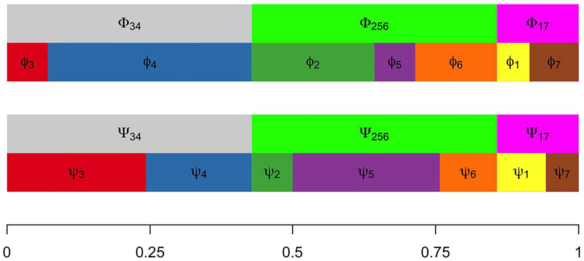
Proportions of $K=7$ cellular subtypes in two different conditions. Aggregated proportions of subtypes 3 and 4, subtypes 2, 5 and 6 and subtypes 1 and 7 remain same across conditions, while individual subtype frequencies change. Depending on the changes in average expression among subtypes, these frequency changes may or may not induce changes between two conditions in the marginal distribution of some gene’s expression.

For any partition $\pi =\left\{b\right\}$, consider aggregate subtype frequencies

$${\Phi }_b=\sum _{k\in b}{\varphi }_k{\text{ and }\Psi }_b=\sum _{k\in b}{\psi }_k$$

and extend the notation, allowing vectors ${\Phi }_{\pi }=\left\{{\Phi }_b:b\in \pi \right\}$, and similarly for ${\Psi }_{\pi }$. Recall the partial ordering of partitions based on refinement, and note that as long as $\pi$ is not the most refined partition (every cell type is in its own block), then the mapping from $\left(\varphi ,\psi \right)$ to $\left({\Phi }_{\pi },{\Psi }_{\pi }\right)$ is many-to-one. Further, define sets

$$A_{\pi }=\left\{\theta \in \Theta :{\Phi }_b={\Psi }_b\forall b\in \pi \right\}$$ (3)

and

$$M_{g,\pi }=\left\{\theta \in \Theta :{\mu }_{g,k}={\mu }_{g,k^{\prime }}\iff k,k^{\prime }\in b,b\in \pi \right\}.$$ (4)

Under $A_{\pi }$ there are constraints on cell subtype frequencies; under $M_{g,\pi }$ there is equivalence in the gene-level distribution of expression between certain subtypes. These sets are precisely the structures needed to address differential distribution ${\text{DD}}_g$ (and its complement, equivalent distribution, ${\text{ED}}_g$) at a given gene $g$.

Theorem 1. Let $C_{g,\pi }=A_{\pi }\cap M_{g,\pi }$. For partitions ${\pi }_1\ne {\pi }_2,C_{g,{\pi }_1}\cap C_{g,{\pi }_2}=\varnothing$. Further, at any gene $g$, equivalent distribution is

$${\text{ED}}_g=\underset{\pi \in \Pi }{\cup }{C}_{g,\pi }.$$

With additional probability structure on the parameter space, we immediately obtain from Theorem 1 a formula for local false discovery rates,

$$1-P\left({\text{DD}}_g\mid X,y\right)=P\left({\text{ED}}_g\mid X,y\right)=\sum _{\pi \in \Pi }P\left(A_{\pi }\cap M_{g,\pi }\mid X,y\right).$$ (5)

Local false discovery rates are important empirical Bayesian statistics in large-scale testing (Efron (2007); Muralidharan (2010); Newton et al. (2004)). For example, the conditional false discovery rate of a list of genes is the arithmetic mean of the associated local false discovery rates. The partition representation guides the construction of a prior distribution (Section 2.3) and a model-based method (Section 2.2) for scoring differential distribution. Setting the stage, Figure 3 shows the dependency structure of the proposed compositional model and the partition-reliant prior specification.

Fig. 3.

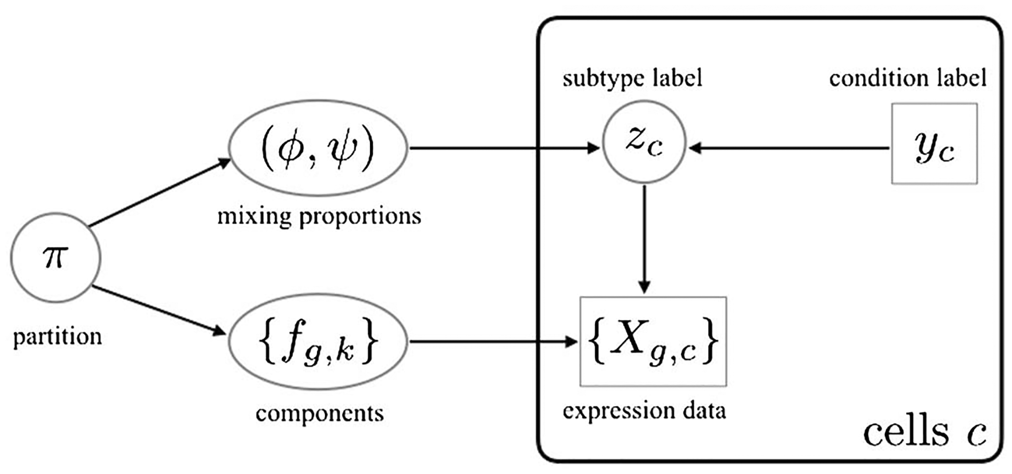
Directed acyclic graph structure of the compositional model and partition-reliant prior. The plate on the right side indicates i.i.d. copies over cells c, conditionally on mixing proportions and mixing components. Observed data are indicated in rectangles/squares, and unobserved variables are in circles/ovals.

Key to computing the gene-specific local false discovery rate $P\left({\text{ED}}_g\mid X,y\right)$ is evaluating probabilities $P\left(A_{\pi }\cap M_{g,\pi }\mid X,y\right)$. The dependence structure (Figure 3) implies a useful reduction of this quantity, at least conditionally upon subtype labels $z=\left(z_c\right)$. For each subtype partition $\pi$ and gene $g$,

Theorem 2. $P\left(A_{\pi }\cap M_{g,\pi }\mid X,y,z\right)=P\left(A_{\pi }\mid y,z\right)P\left(M_{g,\pi }\mid X,z\right)$.

In what follows we develop the modeling and computational elements necessary to efficiently evaluate inference summaries (5) taking advantage of Theorems 1 and 2. Roughly, the methodological idea is that subtype labels $z$ have relatively low uncertainty and may be estimated from genome-wide clustering of cells in the absence of condition information $y$. (up to an arbitrary label permutation). We handle the modest uncertainty in $z$ through a computationally efficient randomized clustering scheme. Theorem 2 indicates that our computational task then separates into two parts given $z$. On one hand, cell subtype frequcies combine with condition labels to give $P\left(A_{\pi }\mid y,z\right)$. Then, gene-level data locally drive the posterior probabilities $P\left(M_{g,\pi }\mid X,z\right)$ that measure differential expression between subtypes. Essentially, the model provides a specific form of information sharing between genes that leverages the compositional structure of single-cell data in order to sharpen our assessments of between-condition expression changes.

2.2. Method structure and clustering.

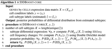
To infer subtypes, we leverage the extensive research on how to cluster cells using scRNA-seq data: for example, SC3 (Kiselev et al. (2017)), CIDR (Lin, Troup and Ho (2017)) and ZIFA (Pierson and Yau (2015)). We propose distance-based clustering on the full set of profiles in a way that is blind to the condition label vector $y$ in order to have as many cells as possible to inform the subtype structure. We investigated several clustering schemes in numerical experiments and allow flexibility in this choice within the scDDboost software. Associating clusters with subtype labels ${\hat{z}}_c$ estimates the actual subtypes $z_c$ and prepares us to use Theorems 1 and 2 in order to compute separate posterior probabilities $P\left(A_{\pi }\mid y,\hat{z}\right)$ and $P\left(M_{g,\pi }\mid X,\hat{z}\right)$ that are necessary for scoring differential distribution. The first probability concerns patterns of cell counts over subtypes in the two conditions and has a convenient closed form within the double-Dirichlet model (Section 2.3). The second probability concerns patterns of changes in expected expression levels among subtypes, and this is also conveniently computed for negative-binomial counts using EBSeq (Leng et al. (2013)). Algorithm 1 summarizes how these elements combine to get the posterior probability of differential distribution per gene, conditional on an estimate of the subtype labels.

We invoke $K$-medoids (Kaufman and Rousseeuw (1987)) as the default clustering method in scDDboost, and customize the cell-cell distance by integrating two measures. The first assembles gene-level information by cluster-based-similarity partitioning (Strehl and Ghosh (2003)). Separately at each gene, modal clustering (Dahl (2009) and in the Supplementary Material Section 2.2, Ma et al. (2021)) partitions the cells, and then we define dissimilarity between cells as the Manhattan distance between gene-specific partition labels. A second measure defines dissimilarity by one minus the Pearson correlation between cells, which is computationally inexpensive, less sensitive to outliers than Euclidean distance and effective at detecting cellular clusters in scRNA-seq (Kim et al. (2019)). The default clustering in scDDboost combines these two measures by weighted average, with $w_C=\frac{{\sigma }_P}{{\sigma }_C+{\sigma }_P}$ and $w_P=1-w_C$, where $w_C,{\sigma }_C,w_P,{\sigma }_P$ are the weights and standard deviations of cluster-based distance and Pearson-correlation distance, respectively. The software allows other distances, such as provided by SC3, which we use in some numerical experiments; in any case, the final distance matrix is denoted $D=\left(d_{i,j}\right)$.

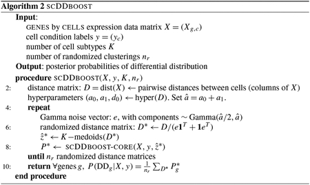
Any clustering method entails classification errors, and so ${\hat{z}}_c\ne z_c$ for some cells. To mitigate the effects of this uncertainty, scDDboost averages output probabilities from scDDboost-core over randomized clusterings ${\hat{z}}^{\text{*}}$. These are not uniformly random but rather are generated by applying $K$-medoids to a randomized distance matrix $D^{\text{*}}=\left(d_{i,j}/w_{i,j}\right)$, where $w_{i,j}$ are nonnegative weights $w_{i,j}=\left(e_i+e_j\right)$, where $\left(e_i\right)$ are independent and identically Gamma distributed deviates with shape $\hat{a}/2$ and rate $\hat{a}$ and where $\hat{a}$ is estimated from $D$. (Thus, $w_{i,j}$ is $\text{Gamma}\left(\hat{a},\hat{a}\right)$ and has unit mean.) The distribution of clusterings induced by this simple computational scheme approximates a Bayesian posterior analysis, as we argue in the Appendix where we also present pseudo-code for the resulting scDDboost Algorithm 2. Averaging over results from randomized clusterings gives additional stability to the posterior probability statistics (Supplementary Figure S10).

Computations become more intensive the larger is the number $K$ of cell subtypes. Version 1.0 of scDDboost is restricted to $K\le 9$; we consider further computational strategies in Section 5. Inferentially, taking $K$ to be too large may inflate the false positive rate (Supplementary Figure S11). The approach taken in ScDDboost is to set $K$ using the validity score (Ray and Turi (2000)) which measures changes in within-cluster sum of squares as we increase $K$. Our implementation, in Supplementary Material Section 2.2, Ma et al. (2021), shows good operating characteristics in simulation.

2.3. $P\left(A_{\pi }\mid y,z\right)$.

We introduce the double Dirichlet mixture (DDM), which is the partition-reliant prior $p\left(\varphi ,\psi \right)$ indicated in Figure 3, in order to derive an explicit formula for $P\left(A_{\pi }\mid y,z\right)$. We lose no generality here by defining $A_{\pi }=\left\{\left(\varphi ,\psi \right):{\Phi }_b={\Psi }_b\forall b\in \pi \right\}$ rather than as a subset of the full parameter space, as in (3). Each $A_{\pi }$ is closed and convex subset of the product space holding all possible pairs of length- $K$ probability vectors.

We propose a spike-slab-style mixture prior with the following form:

$$p\left(\varphi ,\psi \right)=\sum _{\pi \in \Pi }{\omega }_{\pi }{p}_{\pi }\left(\varphi ,\psi \right).$$ (6)

Each mixture component $p_{\pi }\left(\varphi ,\psi \right)$ has support $A_{\pi }$; the mixing proportions ${\omega }_{\pi }$ are positive constants summing to one. To specify component $p_{\pi }$, notice that on $A_{\pi }$ there is a 1–1 correspondence between pairs $\left(\varphi ,\psi \right)$ and parameter states,

$$\left\{\left({\tilde{\varphi }}_b,{\tilde{\psi }}_b,{\Phi }_b\right),\forall b\in \pi \right\},$$ (7)

where

$${\tilde{\varphi }}_b=\frac{{\varphi }_b}{{\Phi }_b},{\tilde{\psi }}_b=\frac{{\psi }_b}{{\Psi }_b}{\text{ and }\Phi }_b=\sum _{k\in b}{\varphi }_k=\sum _{k\in b}{\psi }_k={\Psi }_b$$

For example, ${\tilde{\varphi }}_b$ is a vector of conditional probabilities for each subtype, given that a cell from the first condition is one of the subtypes in $b$.

We introduce hyperparameters ${\alpha }_k^1,{\alpha }_k^2>0$ for each subtype $k$ and set ${\beta }_b={\sum }_{k\in b}\left({\alpha }_k^1+{\alpha }_k^2\right)$ for any possible block $b$. Extending notation, let ${\alpha }_b^j$ be the vector of ${\alpha }_k^j$ for $k\in b,{\beta }_{\pi }$ be the vector of ${\beta }_b$ for $b\in \pi ,{\varphi }_b$ and ${\psi }_b$ be vectors of ${\varphi }_k$ and ${\psi }_k$, respectively, for $k\in b$, and ${\Phi }_{\pi }$ and ${\Psi }_{\pi }$ be the vectors of ${\Phi }_b$ and ${\Psi }_b$ for $b\in \pi$. The proposed double-Dirichlet component $p_{\pi }$ is determined in the transformed scale by assuming ${\Psi }_{\pi }={\Phi }_{\pi }$ and further,

$$\begin{array}{ll}{\Phi }_{\pi }~{\text{Dirichet}}_{N\left(\pi \right)}\left[{\beta }_{\pi }\right],\hfill & \hfill \\ {\tilde{\varphi }}_b~{\text{Dirichlet}}_{N\left(b\right)}\left[{\alpha }_b^1\right]\hfill & \forall b\in \pi ,\hfill \\ {\tilde{\psi }}_b~{\text{Dirichlet}}_{N\left(b\right)}\left[{\alpha }_b^2\right]\hfill & \forall b\in \pi ,\hfill \end{array}$$ (8)

where $N\left(\pi \right)$ is the number of blocks in $\pi$ and $N\left(b\right)$ is the number of subtypes in $b$ and where all random vectors in (8) are mutually independent. Mixing over $\pi$ as in (6), we write $\left(\varphi ,\psi \right)~\text{DDM}\left[\omega =\left({\omega }_{\pi }\right),{\alpha }^1=\left({\alpha }_k^1\right),{\alpha }^2=\left({\alpha }_k^2\right)\right]$.

We record some properties of the component distributions $p_{\pi }$.

Property 1. In $p_{\pi }\left(\varphi ,\psi \right),\psi$ and $\varphi$ are dependent, unless $\pi$ is the null partition in which all subtypes constitute a single block.

Property 2. With $k\in b$, marginal means are

$$E_{\pi }\left({\varphi }_k\right)=\frac{{\alpha }_k^1}{{\sum }_{k^{\prime }\in b}{\alpha }_{k^{\prime }}^1}\frac{{\beta }_b}{{\sum }_{b^{\prime }\in \pi }{\beta }_{b^{\prime }}}\text{ and }{E}_{\pi }\left({\psi }_k\right)=\frac{{\alpha }_k^2}{{\sum }_{k^{\prime }\in b}{\alpha }_{k^{\prime }}^2}\frac{{\beta }_b}{{\sum }_{b^{\prime }\in \pi }{\beta }_{b^{\prime }}}.$$

Recall from (1) the vectors $t^1$ and $t^2$ holding counts of cells in each subtype in each condition, computed from $y$ and $z$. Relative to a block $b\in \pi$, let $t_b^j={\sum }_{k\in b}{t}_k^j$, for cell conditions $j=1,2$, and, let $t_{\pi }^j$ be the vector of these counts over $b\in \pi$. The following properties refer to marginal distributions in which $\left(\varphi ,\psi \right)$ have been integrated out of the joint distribution involving (2) and the component $p_{\pi }$.

Property 3. $t^1$ and $t^2$ are conditionally independent, given $y,t_{\pi }^1$ and $t_{\pi }^2$.

Property 4. For $j=1,2$,

$$p_{\pi }\left(t^j\mid t_{\pi }^j,y\right)=\prod _{b\in \pi }\left\{\left[\frac{\Gamma \left(t_b^j+1\right)}{{\prod }_{k\in b}\Gamma \left(t_k^j+1\right)}\right]\left[\frac{\Gamma \left({\sum }_{k\in b}{\alpha }_k^j\right)}{{\prod }_{k\in b}\Gamma \left({\alpha }_k^j\right)}\right]\left[\frac{{\prod }_{k\in b}\Gamma \left({\alpha }_k^j+t_k^j\right)}{\Gamma \left(t_b^j+{\sum }_{k\in b}{\alpha }_k^j\right))}\right]\right\}.$$

Property 5.

$$p_{\pi }\left(t_{\pi }^1,t_{\pi }^2\mid y\right)=\left[\frac{\Gamma \left(n_1+1\right)\Gamma \left(n_2+1\right)}{{\prod }_{b\in \pi }\Gamma \left(t_b^1+1\right)\Gamma \left(t_b^2+1\right)}\right]\left[\frac{\Gamma \left({\sum }_{b\in \pi }{\beta }_b\right)}{{\prod }_{b\in \pi }\Gamma \left({\beta }_b\right)}\right]\left[\frac{{\prod }_{b\in \pi }\Gamma \left({\beta }_b+t_b^1+t_b^2\right)}{\Gamma \left(n_1+n_2+{\sum }_{b\in \pi }{\beta }_b\right)}\right].$$

Let’s look at some special cases to dissect this result.

Case 1. If $\pi$ has a single block equal to the entire set of cell types $\left\{1,2,\dots ,K\right\}$, then $t_b^j=n_j$ for both $j=1,2$, and Property 5 reduces, correctly, to $p_{\pi }\left(t_{\pi }^1,t_{\pi }^2\mid y\right)=1$. Further,

$$p_{\pi }\left(t^j\mid t_{\pi }^j,y\right)=\left[\frac{\Gamma \left(n_j+1\right)}{\Gamma \left(n_j+{\sum }_{k=1}^K{\alpha }_k^j\right)}\right]\left[\frac{\Gamma \left({\sum }_{k=1}^K{\alpha }_k^j\right)}{{\prod }_{k=1}^K\Gamma \left({\alpha }_k^j\right)}\right]\left[\prod _{k=1}^K\frac{\Gamma \left({\alpha }_k^j+t_k^j\right)}{\Gamma \left(t_k^j+1\right)}\right]$$

which is the well-known Dirichlet-multinomial predictive distribution for counts $t^j$ (Wagner and Taudes (1986)). For example, taking ${\alpha }_k^j=1$ for all types $k$, we get the uniform distribution

$$p_{\pi }\left(t^j\mid t_{\pi }^j,y\right)=\frac{\Gamma \left(n_j+1\right)\Gamma \left(K\right)}{\Gamma \left(n_j+K\right)}.$$

Case 2. At the opposite extreme, $\pi$ has one block $b$ for each class $k$, so $\varphi =\psi$. Then, $p_{\pi }\left(t^j\mid t_{\pi }^j,y\right)=1$, and, further, writing $b=k$,

$$p_{\pi }\left(t_{\pi }^1,t_{\pi }^2\mid y\right)=\left[\frac{\Gamma \left(n_1+1\right)\Gamma \left(n_2+1\right)}{{\prod }_{k=1}^K\Gamma \left(t_k^1+1\right)\Gamma \left(t_k^2+1\right)}\right]\left[\frac{\Gamma \left({\sum }_{k=1}^K{\beta }_k\right)}{{\prod }_{k=1}^K\Gamma \left({\beta }_k\right)}\right]\left[\frac{{\prod }_{k=1}^K\Gamma \left({\beta }_k+t_k^1+t_k^2\right)}{\Gamma \left(n_1+n_2+{\beta }_k\right)}\right],$$

which corresponds to Dirichlet-multinomial predictive distribution for counts $t^1+t^2$ since $t^1$ and $t^2$ are identical distributed given $\left(\varphi ,\psi \right)$ in this case. These properties are useful in establishing

Theorem 3. DDM is conjugate to multinomial sampling of $t^1$ and $t^2$,

$$\left(\varphi ,\psi \right)\mid y,z~\text{DDM}\left[{\omega }^{\text{post}}=\left({\omega }_{\pi }^{\text{post}}\right),{\alpha }^1+t^1,{\alpha }^2+t^2\right]$$

where

$${\omega }_{\pi }^{\text{post}}\propto p_{\pi }\left(t^1\mid t_{\pi }^1,y\right)p_{\pi }\left(t^2\mid t_{\pi }^2,y\right)p_{\pi }\left(t_{\pi }^1,t_{\pi }^2\mid y\right){\omega }_{\pi }$$ (9)

The target probability $P\left(A_{\pi }\mid y,z\right)$ is an integral of the posterior distribution in Theorem 3. To evaluate it, we need to contend with the fact that sets $\left\{A_{\pi }:\pi \in \Pi \right\}$ are not disjoint. Relevant overlaps have to do with partition refinement. Recall that a partition ${\pi }^r$ is a refinement of a partition ${\pi }^c$ if, for any $b\in {\pi }^c$, there exists $s\subset {\pi }^r$ such that ${\cup }_{b^{\prime }\in s}{b}^{\prime }=b$. We say ${\pi }^c$ coarsens ${\pi }^r$ when ${\pi }^r$ refines ${\pi }^c$. Any partition both refines and coarsens itself as a trivial case. Generally, refinements increase the number of blocks. If subtype frequency vectors $\left(\varphi ,\psi \right)$ satisfy the constraints in $A_{{\pi }^r}$, then they also satisfy the constraints of any ${\pi }^c$ that coarsens ${\pi }^r$; that is, $A_{{\pi }^r}\subset A_{{\pi }^c}$. Refinements reduce the dimension of allowable parameter states. For the double-Dirichlet component distributions $P_{\pi }$, we find

Property 6. For two partitions $\tilde{\pi }$ and $\pi ,P_{\tilde{\pi }}\left(A_{\pi }\mid y,z\right)=1[\tilde{\pi }$ refines $\pi ]$.

This supports the main finding of this section,

$$P\left(A_{\pi }\mid y,z\right)=\sum _{\tilde{\pi }\in \Pi }{\omega }_{\tilde{\pi }}^{\text{post}}1\left[\tilde{\pi }\text{ refines }\pi \right]$$ (10)

2.4. $P\left(M_{g,\pi }\mid X,z\right)$.

We leverage well-established modeling techniques for transcript analysis, including (Leng et al. (2013), Newton and Kendziorski (2003) and Jensen et al. (2009)) which characterize equivalent or differential expression in terms of shared or independently drawn mean effects. Let $X_{g,b}$ denote the subvector of expression values at gene $g$ over cells $c$ with $z_c=k$ for which subtype $k$ is part of block $b$ of partition $\pi$. Conditioning on subtype labels $z=\left(z_c\right)$, we assume that under $M_{g,\pi }$ :

1. Between blocks: subvectors $\left\{X_{g,b}:b\in \pi \right\}$ are mutually independent;

2. Within blocks: for cells mapping to block $b$, observations $X_{g,c}$ are i.i.d;

3. Mean effects: for each block $b$, there is a univariate mean, ${\mu }_{g,b}$, shared by cells mapping to that block; a priori these means are i.i.d. between blocks.

These assumptions imply a useful factorization marginally to latent means,

$$P\left(X_g\mid M_{g,\pi },z\right)=\prod _{b\in \pi }f\left(X_{g,b}\right),$$ (11)

where $f$ is a customized density kernel. In our case we use EBseq from (Leng et al. (2013)): the sampling distribution of $X_{g,c}$ is negative binomial, and $f$ becomes a particular compound multivariate negative binomial formed from integrating uncertainty in the block-specific means (see Supplementary Material Section 2.2, Ma et al. (2021)). Through its gene-level mixing model, EBseq also gives estimates of $\left\{P\left(M_{g,\pi }\mid z\right)\right\}$ : the proportions of genes governed by any of the different patterns $\pi$ of equivalent/differential expression among subtypes. With these estimates and (11) we compute by Bayes’s rule,

$$P\left(M_{g,\pi }\mid X,z\right)\propto P\left(M_{g,\pi }\mid z\right)\prod _{b\in \pi }f\left(X_{g,b}\right).$$

The proportionality is resolved by calculating over all partitions $\pi$.

3. Numerical experiments.

3.1. Synthetic data.

We used splatter (v. 1.2.0) to generate synthetic scRNA-seq data for which the DD status of genes is known (Zappia, Phipson and Oshlack (2017)), thereby allowing us to measure operating characteristics of scDDboost in a controlled setting. Splatter is a generative system for simulating realistic single-cell RNA-seq data. It accounts for biological and technical sources of variation and is calibrated from a number of published data sets. Our hypothetical two-condition comparison involved $n=400$ cells and 17,421 genes and mixing over various numbers $K$ of distinct subtypes. To reflect common variation patterns, we adopted default settings of the primary parameters in splatter and focused our experiments on four settings of splatter’s location and scale parameters $\left(\theta ,\gamma \right)$ which encode distributional shifts between subtypes. We entertained 12 scenarios encoding four distributional shift settings for each of three different values for the number $K$ of subtypes, with composition parameters $\varphi$ and $\psi$ selected to account for various mixing possibilities. Ten replicate data sets were simulated on each scenario. These 12 scenarios, encoded by $K/\theta /\gamma$, span states with rather strong signals, like 3/ −0.1/1 to quite weak signals, like 15/0.1/0.4. Supplementary Figures S6 and S7 provide a view of the global separation between the subtypes and the degree of difficulty of the inference task. We note that the mechanistic sampling model induced by splatter is distinct from the descriptive model underlying scDDboost. We choose it to reflect anticipated technical and biological sources of variation. Further details are in Supplementary Material Section 3.1, Ma et al. (2021).

Figures 4 and 5 summarize the true positive rate and false discovery rate of scDDboost compared to three other methodologies: MAST (v. 1.4.0), ScDD (v. 1.2.0) and DESeq2 (v. 1.18.1). scDDboost exhibits very good operating characteristics in this study, as it controls the FDR in all cases while also delivering a relatively high rate of true positives in all cases. The beneficial sampling properties are not limited to the 5% FDR threshold, as indicated by receiver operator characteristic curves (Supplementary Figure S9).

Fig. 4.

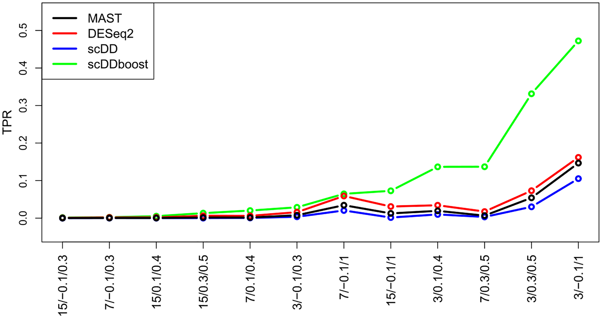
True positive rate (vertical) of four DD detection methods in 12 synthetic-data settings (horizontal). Settings are labeled for $K/\theta /\gamma$ and ranked by scDDboost values. Each method is targeting a 5% false discovery rate (FDR). The plot shows average rates over replicate simulated data in each setting.

Fig. 5.

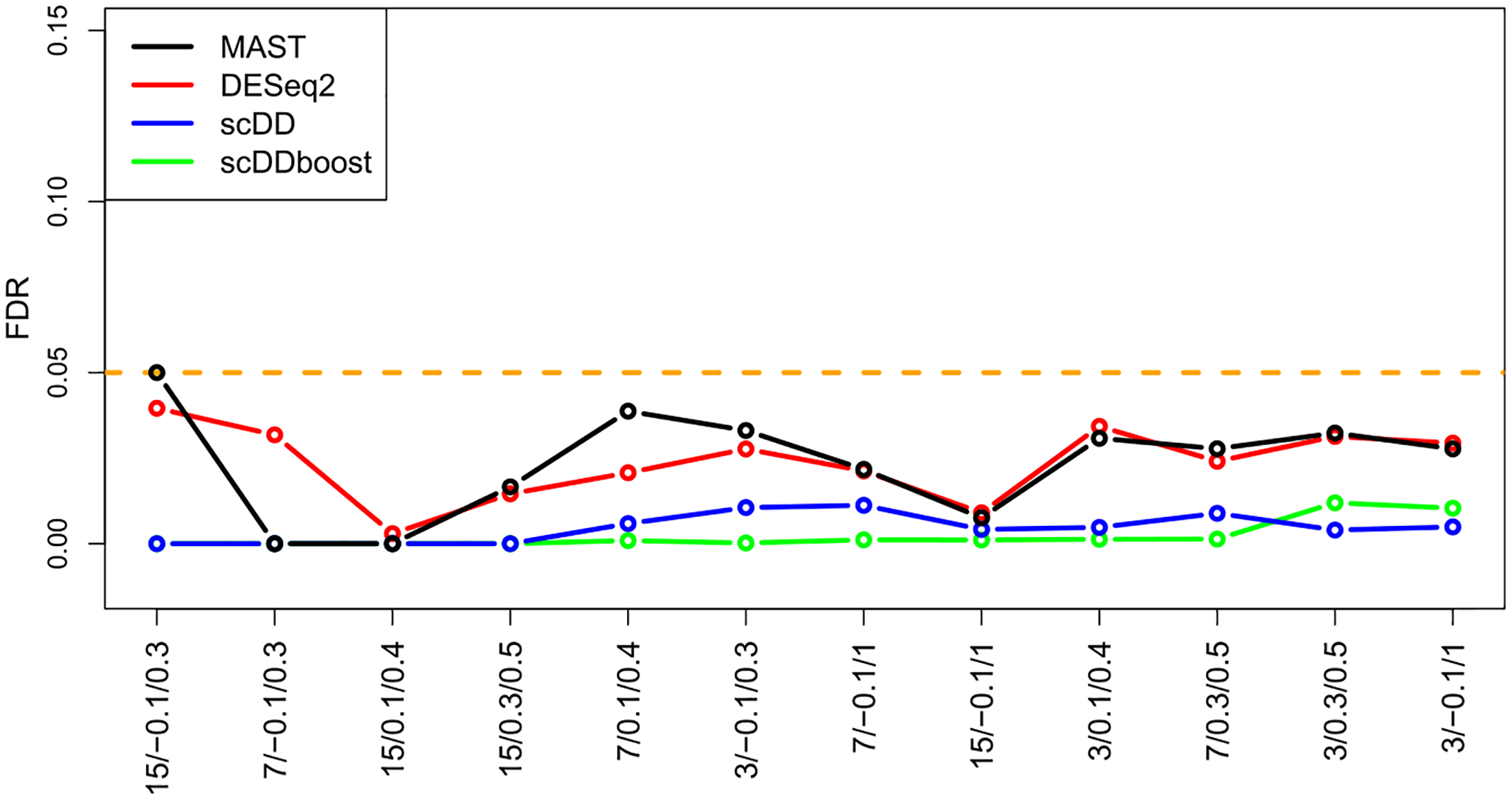
False discovery rate (vertical) of methods in the synthetic-data settings (horizontal, same order) from Figure 4. FDR is approximated from the 12 replicate data sets in each scenario using the known generative hypothesis states.

3.2. Empirical study.

We applied scDDboost to a collection of previously published data sets that are recorded at conquer (Soneson and Robinson (2018)). Though not knowing the truly DD genes, we can examine how scDDboost output compares to output from several standard methods. We selected 12 data sets from conquer representing different species and experimental settings and involving hundreds to thousands of cells. Appendix Table A1 provides details. Figure 6 compares methods in terms of the size of the reported list of DD genes at the 5% FDR target level. We see a consistently high yield of scDDboost among the evaluated methods. For reference, one of these data sets (GSE64016) happens to be the data behind Figure 1, where we know from other information that some of the uniquely identified genes are likely not to be false positives.

Fig. 6.

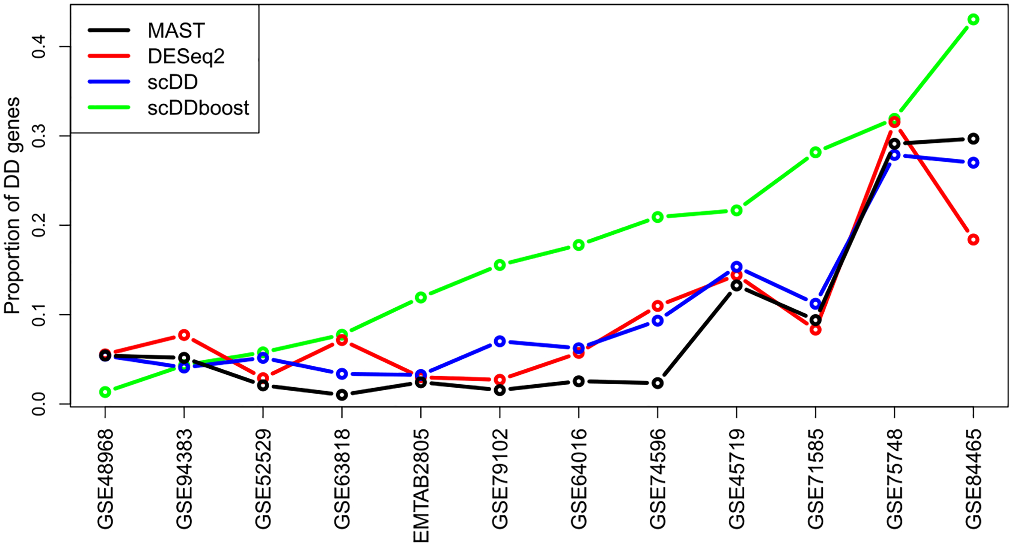
Proportion of DD genes at 5% FDR threshold with respect to total number of genes identified by each method. Data sets are ordered by scDDboost list size.

To check that the increased discovery rate of scDDboost is not associated with an increased rate of false calls, we applied it to a series of random splits of single-condition data sets (Appendix Table A2). Figure 7 confirms a very low call rate in cases where no changes in distribution are expected.

Fig. 7.

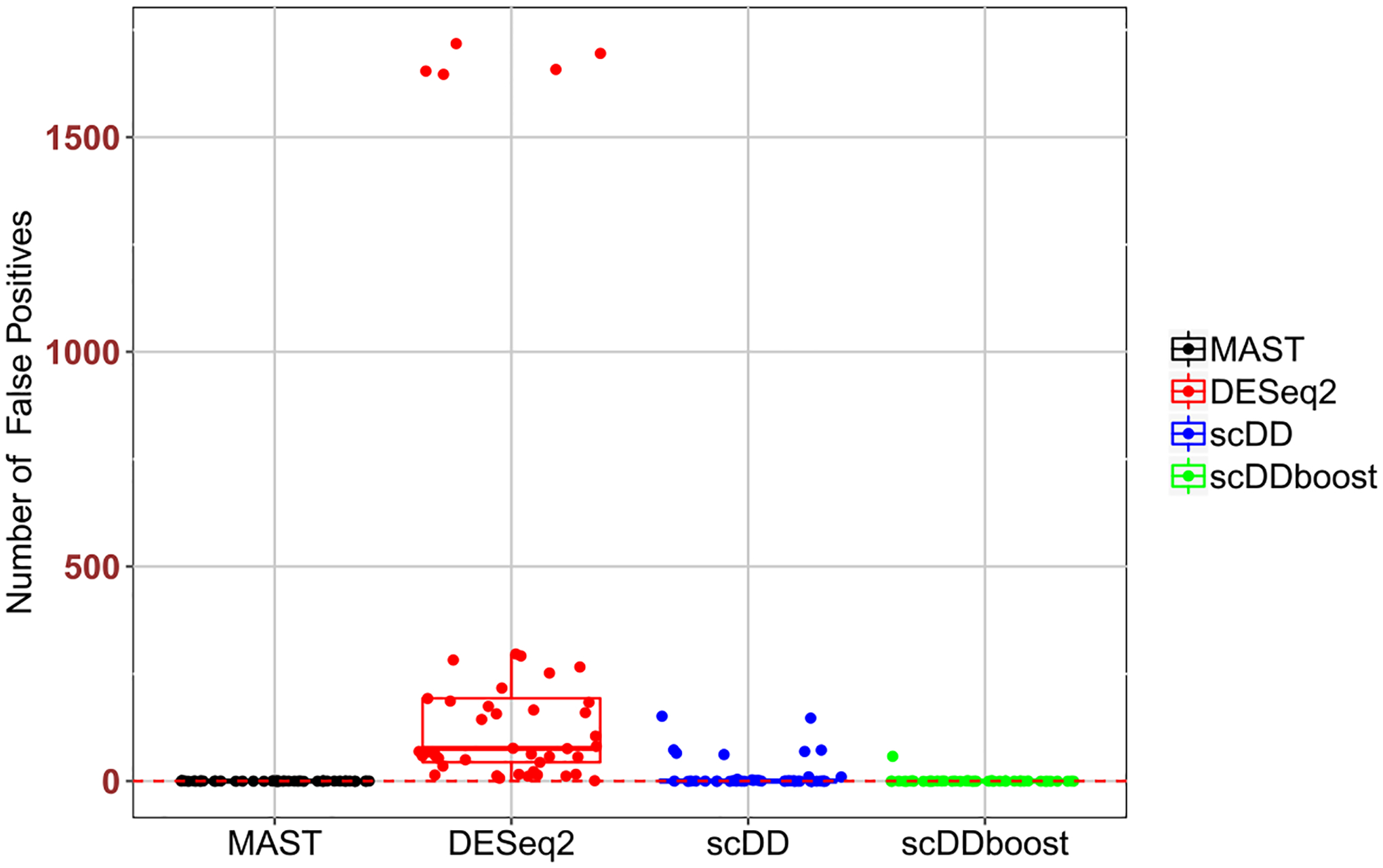
False positive counts at 5% FDR threshold by several methods on five random splits of nine single-condition data sets from Appendix Table A2.

We conjecture that scDDboost gains power through its novel approach to borrowing strength across genes, that is, that the genomic data are providing information about cell subtypes and mixing proportions, leaving gene-level data to guide gene-specific mixture components. One way to drill into this idea is to consider how many genes have similar expression characteristics to a given gene. By virtue of the EBseq analysis inside scDDboost, we may assign each gene to a set of related genes that all have the same highest-probability pattern of equality/inequality of means across the subtypes. Say ${\hat{\pi }}_g={\text{argmax}}_{\pi }P\left(M_{g,\pi }\mid \hat{z},X\right)$. In Figure 8 we show that, compared to DD genes commonly identified by multiple methods (blue), the set sizes for genes uniquely identified by scDDboost (red) tend to be larger. Essentially, the proposed methodology boosts weak DD evidence when a gene’s pattern of differential expression among cell subtypes matches a large number of other genes.

Fig. 8.

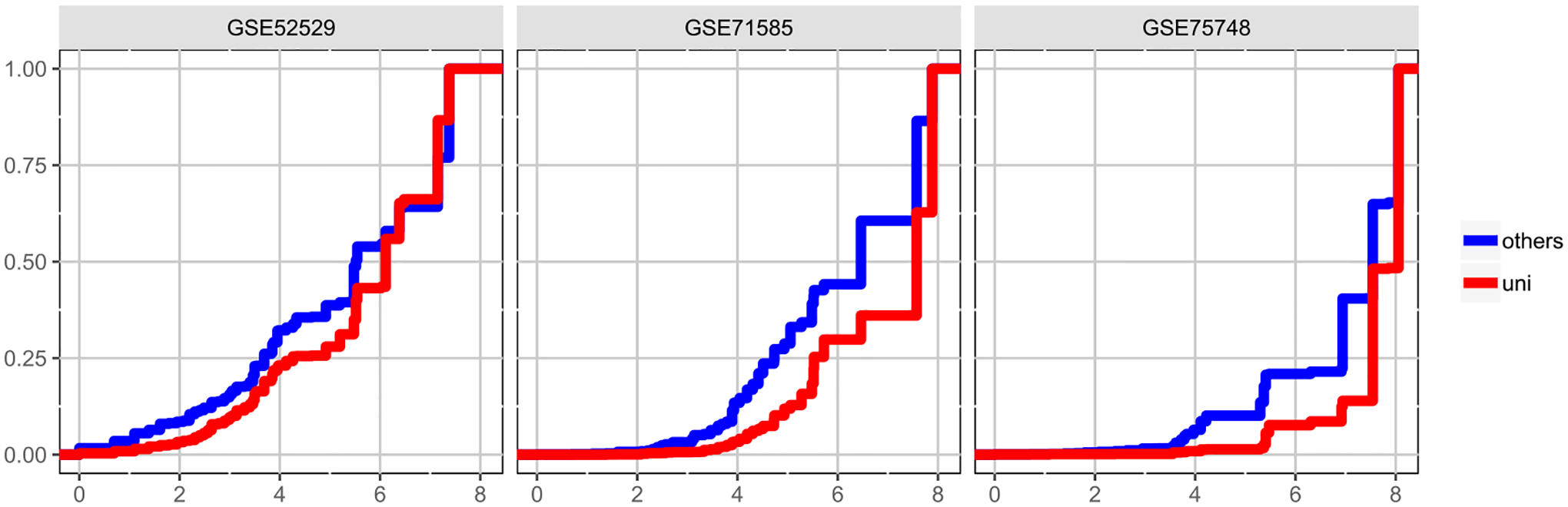
Genes are grouped by their pattern of differential expression across subtypes as inferred by the EBseq computation within scDDboost for three example datasets. Cumulative distribution functions of the log-scale size statistic for all genes identified by scDDboost are plotted; red is the subset uniquely identified by scDDboost; blue are those also identified by the comparison methods (MAST, scDD, or DESeq2). Sets of similarly-patterned genes tend to be larger (horizontal axis, log size) for genes uniquely identified by scDDboost (red) compared to other DD genes (blue), at 5% FDR.

3.3. Bursting.

Transcriptional bursting is a fundamental property of genes, wherein transcription is either negligible or attains a certain probability of activation (Raj and van Oudenaarden (2008)). D3E (Delmans and Hemberg (2016)) is a computationally intensive method for DE gene analysis rooted in modeling the bursting process. It considers transcripts as in the stationary distribution from an experimentally validated stochastic process of single-cell gene expression (Peccoud and Ycart (1995)). Three mechanistic parameters (rate of promoter activation, rate of promoter inactivation and the conditional rate of transcription given an active promoter) characterize the model which allows distributional changes between conditions without changes in mean expression level. For genes identified as DD by scDDboost in dataset GSE71585, either uniquely or in common with comparison methods MAST, scDD and DESeq2, Figure 9 shows changes of these bursting parameters. Interestingly, genes uniquely identified by scDDboost are associated with more significant changes between estimated bursting parameters than genes that all methods identify. This finding and similar findings on other data sets (not shown) provide some evidence that scDDboost is able to detect biologically meaningful changes in the expression distribution.

Fig. 9.

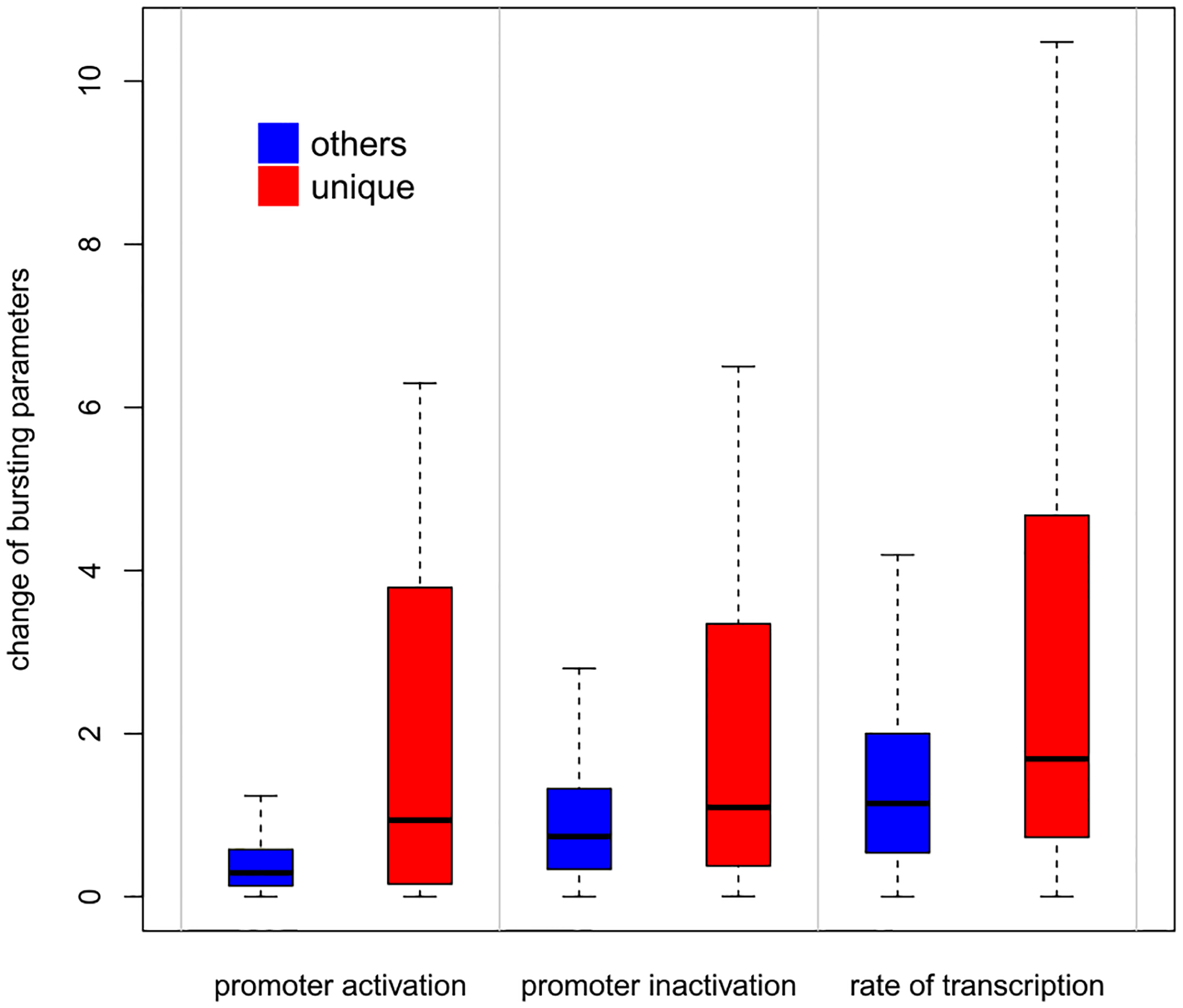
Absolute values of log fold changes of bursting parameters tend to be larger for 1758 genes uniquely identified by scDDboost (red) compared to 2983 genes (blue) that are identified at 5% FDR by scDDboost and other methods: MAST, scDD, and DESeq2.

3.4. Time complexity.

Run time complexity of scDDboost is dominated by the cost of clustering cells and of running EBSeq to measure differences between subtypes. Recall the notation that $n$ for number of cells, $G$ for number of genes and $K$ for number of subtypes. Our distance-based clustering of $n$ cells measuring $G$ genes requires on the order of $G\times n^2$ operations (see Supplementary Material Section 2.2, Ma et al. (2021)). Further, EBSeq uses summed counts within each subtype for each gene to compute its density kernel, and there are $\text{Bell}\left(K\right)$ differential patterns to compute, where Bell counts the partitions of $K$. We impose the computational limit $K\le 9$ in scDDboost (v. 1.0). In a typical case involving 20,000 genes and 200 cells, using 50 of randomized distances, scDDboost is relatively efficient for $K\le 6$ requiring less than 15 CPU minutes on, for example, a quad-core 2.2 GHz Intel Core i7 with 16 Gb of RAM. The same data might require 20 to 40 CPU hours when $K=9$. In Section 5 we mention some opportunities to improve this speed.

3.5. Diagnostics.

As implemented, scDDboost uses a particular distance matrix to inform subtypes and computes probabilities in a model for which expression is a mixture of constant-shape negative binomials. To check the effect of these assumptions, we consider a variety of diagnostic calculations using the data sets presented in Sections 3.1 and 3.2. We first point out that model misspecification may have a limited impact on Type-I error rates, as evidenced by the permutation study (Figure 7) and also the synthetic-data study (Figure 5), which does not encode the same modeling assumptions as scDDboost.

To check the within-subtype negative binomial (NB) assumption, we deployed a bootstrap goodness-of-fit test in three data sets (Yin and Ma (2013)). Fewer than 1.5% of genes show evidence against a within subtype NB assumption at a 5% FDR. Further, for most of these non-NB genes the inference drawn by scDDboost is the same as that drawn by various other methods (Supplementary Table S3) and where there are differences the scDDboost call is plausible (Supplementary Figure S12). Among the genes identified by scDDboost at 5% FDR in the stem-cell example (recall Figure 1), just six of them fail the NB test, and two of these are uniquely called by scDDboost; further, one of the two genes is cell-cycle related.

The constant-shape assumption is less well supported empirically, according to a likelihood-ratio test that we developed (Supplementary Figure S13). More than 15% of genes show evidence against constant shape in the examples considered, though inference on differential distribution is only mildly affected (Supplementary Table S4, Figure S14). We have similar findings in the splatter-generated synthetic data. Even with evident model misspecification, Figure 10 shows that the marginal fit by scDDboost is reasonably accurate in the stem-cell example.

Fig. 10.

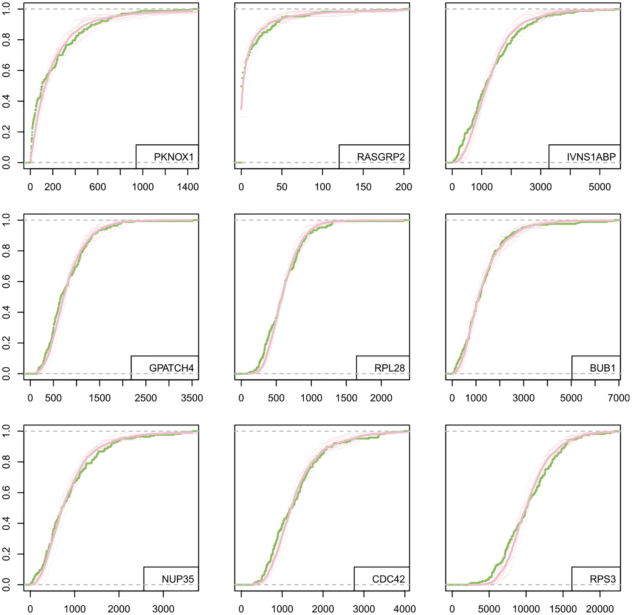
Empirical CDF for observed data (green) compared to expression levels simulated from the fitted NB mixture (pink) for data set GSE64016. The top six panels are genes randomly selected from those genes being identified as DD by scDDboost and not violating constant shape assumption; the last three genes are randomly sampled from genes that fail the test of constant NB shape parameter. Each thin pink curve is from one of the randomized distances; the thicker pink curve represents pointwise averaging over 10 randomized distance matrices. Note, horizontal scales differ among the panels, and cells are pooled from the two conditions.

Choice of distance function.

We propose distance-based clustering to convey subtype information (Section 2.2), and one may ask how sensitive are findings to the choice of distance function. The randomization scheme mitigates variation associated with the specific partition of cells, but the choice of distance function does affect the computed probabilities. To check this, we repeated the numerical experiments in Section 3 using the SC3 distance in place of the default. Importantly, Type I error rates remain in control, as evidenced by the simulation study and the negative-control permutatation study (Supplementary Figure S15). There can be substantial differences in yeild at a given FDR control level (Supplementary Table S5).

4. Asymptotics of the double Dirichlet mixture.

Summary statistics $P\left(A_{\pi }\mid y,z\right)$, from Section 2.3, are amenable to a first-order asymptotic analysis that provides further insight into DDM model behavior. The fact that support sets $A_{\pi }$ for component distributions $p_{\pi }\left(\varphi ,\psi \right)$ are not disjoint becomes an important issue. Consider distinct partitions ${\pi }_1$ and ${\pi }_2$ of subtypes $\left\{1,2,\dots ,K\right\}$, and recall that $N\left(\pi \right)$ counts the number of blocks in partition $\pi$. In case ${\pi }_2$ refines ${\pi }_1$, then $N\left({\pi }_1\right)<N\left({\pi }_2\right)$, and we also know that $A_{{\pi }_2}\subset A_{{\pi }_1}$, since refinement imposes additional constraints on the pair $\left(\varphi ,\psi \right)$ of probability vectors. If the data-generating state $\left(\varphi ,\psi \right)\in A_{{\pi }_2}$, one might ask how posterior probability mass tends to be allocated among the other mixture components whose support sets also contain this state. The question is addressed by the following.

Theorem 4. Let ${\pi }_1$ and ${\pi }_2$ denote two partitions for which $N\left({\pi }_1\right)<N\left({\pi }_2\right)$ and $A_{{\pi }_1}\cap$ $A_{{\pi }_2}$ is nonempty. Let $\left(\varphi ,\psi \right)\in A_{{\pi }_1}\cap A_{{\pi }_2}$ denote the data generating state for subtype labels $z_1,z_2,\dots ,z_n$ given i.i.d. Bernoulli condition labels $y_1,y_2,\dots ,y_n$, and recall the posterior mixing proportions ${\omega }_{\pi }^{\text{post}}$ from equation (9) with hyperparameters ${\alpha }_i^j\ge 1$ for $i=1,\dots ,K$, $j=1,2$. Then

$$\frac{{\omega }_{{\pi }_1}^{\text{post}}}{{\omega }_{{\pi }_2}^{\text{post}}}{\to }_{\text{a.s. }}0\text{ as }n\to \infty .$$

Essentially, mixing mass is transferred to components associated with the most refined partition consistent with a given parameter state. To be precise, let $H\left(\varphi ,\psi \right)=\{\pi :\left(\varphi ,\psi \right)\in A_{\pi }\}$ record all the partitions associated with one state. Typically, there is a most refined partition, ${\pi }^{\text{*}}={\pi }^{\text{*}}\left(\varphi ,\psi \right)$ such that

$$A_{{\pi }^{\text{*}}}=\underset{\pi \in H\left(\varphi ,\psi \right)}{\cap }{A}_{\pi }.$$ (12)

This always happens when $K\le 3$. In Supplementary Material Section 4, Ma et al. (2021), we characterize the exceptional set of states where (12) does not hold. Notably, if (12) does hold for state $\left(\varphi ,\psi \right)$, then, for any $\pi \in H\left(\varphi ,\psi \right)$, using Theorem 4 and (10), we have

$$P\left(A_{\pi }\mid y_1,\dots ,y_n;z_1,\dots ,z_n\right){\to }_{\text{a.s. }}1\text{ as }n\to \infty .$$

This provides conditions under which we expect good performance for large numbers of cells.

5. Concluding remarks.

We have presented scDDboost, a tool for detecting differentially distributed genes from scRNA-seq data, where transcripts are modeled as a mixture of cellular subtypes. The methodology links established model-based techniques with novel empirical Bayesian modeling and computational elements to provide a powerful detection method showing comparatively good operating characteristics in simulation, empirical and asymptotic studies.

In the software and numerical experiments we made specific choices, such as to use mixtures of negative binomial components per gene, and to use K-medoids clustering on particular cell-cell distances. These choices have evident advantages, but the model structure and theory developed in Section 2 carry through for other cases. Future experiments could study other formulations within the same schema; for example there may be cell-cell distances that better capture the intrinsic dimensionality of expression programs, including, perhaps distances based on diffusions (Haghverdi, Buettner and Theis (2015)) or the longest-leg path distance (Little, Maggioni and Murphy (2017)). Future experiments could also further assess operating characteristics when the number of cells is very large and the number of reads is relatively small, as may arise with unique molecular identifiers (Chen et al. (2018)). Further, assuming a compositional structure to drive model-based computations may not be restrictive, since it allows great flexibility in the form of each gene/condition-specific expression distribution (as coded, they are finite mixtures of negative binomials).

EBSeq currently presents a computational bottleneck for scDDboost, since it searches all partitions of $K$ and encodes a hyperparameter estimation algorithm that scales poorly with $K$. Several approximations present themselves that may redress the problem, since, in the mixture model context, only patterns $\pi$ corresponding to relatively probable expression-change patterns over subtypes have a big impact on the final posterior inference Ma, Kendziorski and Newton (2020). Even after resolving this bottleneck, there are advantages to having $K$ small compared to $n$. Numerical experiments show increased false discoveries when $K$ is overestimated. But accurate estimation with large $K$ would not be expected to provide much improved power, since that depends on accurate estimation of subtypes and their frequencies which relies on $K$ being relatively small compared to $n$.

APPENDIX

Proof of Theorem 1. If $\theta \in {\cup }_{\pi \in \Pi }\left[A_{\pi }\cap M_{g,\pi }\right]$, then there exists a partition $\pi$ for which $\theta \in A_{\pi }$ and $\theta \in M_{g,\pi }$. By construction

$$f_g^1\left(x\right)=\sum _{k=1}^K{\varphi }_k{f}_{g,k}\left(x\right)=\sum _{b\in \pi }\sum _{k\in b}{\varphi }_k{f}_{g,k}\left(x\right)=\sum _{b\in \pi }{\Phi }_b{f}_{g,k^{\text{*}}\left(b\right)}\left(x\right),$$

where $k^{\text{*}}\left(b\right)$ indexes any component in $b$, since all components in that block have the same component distribution owing to constraint $M_{g,\pi }$. Continuing, using the constraint $\theta \in A_{\pi }$,

$$f_g^1\left(x\right)=\sum _{b\in \pi }{\Psi }_b{f}_{g,k^{\text{*}}\left(b\right)}\left(x\right)=f_g^2\left(x\right)\forall x$$

That is, $\theta \in {\text{ED}}_g$.

If $\theta \in {\text{ED}}_g$, then $f_g^1\left(x\right)=f_g^2\left(x\right)$ for all $x$. Noting that both are mixtures over the same set of components $\left\{f_{g,k}\right\}$, let $\left\{h_{g,l}:l=1,2,\dots ,L\right\}$ be the set of distinct components over this set, and so

$$f_g^1\left(x\right)=\sum _{k=1}^k{\varphi }_k{f}_{g,k}\left(x\right)=\sum _{l=1}^L{c}_{g,l}\left(\varphi \right)h_{g,l}\left(x\right)=\sum _{l=1}^L{c}_{g,l}\left(\psi \right)h_{g,l}\left(x\right)=f_g^2\left(x\right),$$

where

$$c_{g,l}\left(\varphi \right)=\sum _{k=1}^K{\varphi }_{k}1\left[f_{g,k}=h_{g,l}\right],c_{g,l}\left(\psi \right)=\sum _{k=1}^K{\psi }_{k}1\left[f_{g,k}=h_{g,l}\right].$$ (13)

Finite mixtures of distinct negative binomial components are identifiable (Proposition 5 from Yakowitz and Spragins (1968)), and so the equality of $f_g^1$ and $f_g^2$ implies $c_{g,l}\left(\varphi \right)=c_{g,l}\left(\psi \right)$ for all $l=1,2,\dots ,L$. Identifying the partition blocks $b_l=\left\{k:f_{g,k}=h_{g,l}\right\}$ and the partition $\tilde{\pi }=\left\{b_l\right\}$, we find $\theta \in A_{\tilde{\pi }}\cap M_{g,\tilde{\pi }}$. The accumulated probabilities in (13) correspond to ${\Phi }_{\tilde{\pi }}$ and ${\Psi }_{\tilde{\pi }}$ which are equal on $A_{\tilde{\pi }}$.

Randomizing distances for approximate posterior inference.

One way to frame the subtype problem is to suppose that subtype labels $z=\left(z_i\right)$ satisfy $z=f\left(\Delta \right)$, where $\Delta =\left({\delta }_{i,j}\right)$ is a $n\times n$ matrix holding true, unobservable distances, such as ${\delta }_{i,j}$ between cells $i$ and $j$ and that $f$ is some assignment function, like the one induced by the $K$-medoids algorithm. Then, posterior uncertainty in $z$ would follow directly from posterior uncertainty in $\Delta$. On one hand, we could proceed via formal Bayesian analysis, say under a simple conjugate prior in which $1/{\delta }_{i,j}~\text{Gamma}\left(a_0,d_0\right)$, for hyperparameters $a_0$ and $d_0$ and in which the observed distance $d_{i,j}\mid {\delta }_{i,j}~\text{Gamma}\left(a_1,a_1/{\delta }_{i,j}\right)$. This would assure that ${\delta }_{i,j}$ is the expectation of $d_{i,j}$, with shape parameter $a_1$ affecting variation of measured distances about their expected values. Not accounting for any constraints imposed by both $D$ and $\Delta$ being distance matrices, we would have the posterior distribution $1/{\delta }_{i,j}\mid D~\text{Gamma}\left(a_0+a_1,d_0+a_1{d}_{i,j}\right)$. For any threshold $c>0$, we would find

$$P\left({\delta }_{i,j}\le c\mid D\right)=P\left(U\ge \frac{d_0+a_1{d}_{i,j}}{c\left(a_0+a_1\right)}\right)$$ (14)

where $U~\text{Gamma}\left(a_0+a_1,a_0+a_1\right)$.

Alternatively, we could form randomized distances $d_{i,j}^{\text{*}}=d_{i,j}/w_{i,j}$, where $w_{i,j}$ is the analyst-supplied random weight distributed as $\text{Gamma}\left(\hat{a},\hat{a}\right)$, as in Section 2.2. Notice that

$$P\left(d_{i,j}^{\text{*}}\le c\mid D\right)=P\left(w_{i,j}>d_{i,j}/c\mid D\right)$$

which is also an upper tail probability for a unit-mean Gamma deviate with shape and rate equal to $\hat{a}$. Comparing to (14), by setting $\hat{a}$ to equal $a_0+a_1$, and if $a_0$ and $d_0$ are relatively small, we find

$$P\left(d_{i,j}^{\text{*}}\le c\mid D\right)\approx P\left({\delta }_{i,j}\le c\mid D\right).$$

In other words, the randomized distance procedure is providing approximate posterior draws of the underlying distance matrix. In spite of limitations of this procedure for full Bayesian inference, it provides an elementary scheme to account for uncertainty in subtype allocations. Numerical experiments in the Supplementary Material make comparisons to a full, Dirichlet-process-based, posterior analysis.

Pseudo-code.

Empirical datasets.

Appendix Table A1.

Data sets used for the empirical study of scDDboost

	Conditions	# cells	Organism	Ref
GSE94383	0 min unstim vs 75 min stim	186, 145	human	Lane et al. (2017)
GSE48968-GPL13112	BMDC (2h LPS stimulation) vs 6h LPS	96, 96	mouse	Shalek et al. (2014)
GSE52529	T0 vs T72	69, 74	human	Trapnell et al. (2014)
GSE74596	NKT1 vs NTK2	46, 68	mouse	Engel et al. (2016)
EMTAB2805	G1 vs G2M	96, 96	mouse	Buettner et al. (2015)
GSE71585-GPL13112	Gad2tdTpositive vs Cux2tdTnegative	80, 140	mouse	Tasic et al. (2016)
GSE64016	G1 vs G2	91,76	human	Leng et al. (2015)
GSE79102	patient1 vs patient2	51, 89	human	Kiselev et al. (2017)
GSE45719	16-cell stage blastomere vs mid blastocyst cell	50, 60	mouse	Deng et al. (2014)
GSE63818	Primordial Germ Cells, developmental stage: 7 week gestation vs Somatic Cells, developmental stage: 7 week gestation	40, 26	mouse	Guo et al. (2015)
GSE75748	DEC vs EC	64, 64	human	Chu et al. (2016)
GSE84465	neoplastic cells vs non-neoplastic cells	1000, 1000	human	Darmanis et al. (2017)

Appendix Table A2.

Single-condition data sets used in the random-splitting experiment

Data set	Condition	# cells
GSE63818null	7 week gestation	40
GSE75748null	DEC	64
GSE94383null	T0	186
GSE48968-GPL13112null	BMDC (2h LPS stimulation)	96
GSE74596null	NKT1	46
EMTAB2805null	G1	96
GSE71585-GPL13112null	Gad2tdTpositive	80
GSE64016null	G1	91
GSE79102null	patient1	51

REFERENCES

- Anders S and Huber W (2010). Differential expression analysis for sequence count data. Genome Biol 11 R106. 10.1186/gb-2010-11-10-r106 [DOI] [PMC free article] [PubMed] [Google Scholar]
- Bacher R and Kendziorski C (2016). Design and computational analysis of single-cell RNA-sequencing experiments. Genome Biol 17 63. 10.1186/s13059-016-0927-y [DOI] [PMC free article] [PubMed] [Google Scholar]
- Buettner F, Natarajan KN, Casale FP, Proserpio V, Scialdone A, Theis FJ, Teichmann SA, Marioni JC and Stegle O (2015). Computational analysis of cell-to-cell heterogeneity in single-cell RNA-sequencing data reveals hidden subpopulations of cells. Nat. Biotechnol 33155. [DOI] [PubMed] [Google Scholar]
- Chen W, Li Y, Easton J, Finkelstein D, Wu G and Chen X (2018). UMI-count modeling and differential expression analysis for single-cell RNA sequencing. Genome Biol 19 70. 10.1186/s13059-018-1438-9 [DOI] [PMC free article] [PubMed] [Google Scholar]
- Chu L-F, Leng N, Zhang J, Hou Z, Mamott D, Vereide DT, Choi J, Kendziorski C, Stewart R et al. (2016). Single-cell RNA-seq reveals novel regulators of human embryonic stem cell differentiation to definitive endoderm. Genome Biol 17 173. 10.1186/s13059-016-1033-x [DOI] [PMC free article] [PubMed] [Google Scholar]
- Dahl DB (2009). Modal clustering in a class of product partition models. Bayesian Anal 4 243–264. MR2507363 10.1214/09-BA409 [DOI] [Google Scholar]
- Darmanis S, Sloan SA, Croote D, Mignardi M, Chernikova S, Samghababi P, Zhang Y, Neff N, Kowarsky M et al. (2017). Single-cell RNA-seq analysis of infiltrating neoplastic cells at the migrating front of human glioblastoma. Cell Rep 21 1399–1410. 10.1016/j.celrep.2017.10.030 [DOI] [PMC free article] [PubMed] [Google Scholar]
- Delmans M and Hemberg M (2016). Discrete distributional differential expression (D3E)-A tool for gene expression analysis of single-cell RNA-seq data. BMC Bioinform 17 110. 10.1186/s12859-016-0944-6 [DOI] [PMC free article] [PubMed] [Google Scholar]
- Deng Q, Ramsköld D, Reinius B and Sandberg R (2014). Single-cell RNA-seq reveals dynamic, random monoallelic gene expression in mammalian cells. Science 343 193–196. 10.1126/science.1245316 [DOI] [PubMed] [Google Scholar]
- Dominguez D, Tsai Y-H, Gomez N, Jha DK, Davis I and Wang Z (2016). A high-resolution transcriptome map of cell cycle reveals novel connections between periodic genes and cancer. Cell Res 26 946. [DOI] [PMC free article] [PubMed] [Google Scholar]
- Efron B (2007). Size, power and false discovery rates. Ann. Statist 35 1351–1377. MR2351089 10.1214/009053606000001460 [DOI] [Google Scholar]
- Engel I, Seumois G, Chavez L, Samaniego-Castruita D, White B, Chawla A, Mock D, Vijayanand P and Kronenberg M (2016). Innate-like functions of natural killer T cell subsets result from highly divergent gene programs. Nat. Immunol 17 728. [DOI] [PMC free article] [PubMed] [Google Scholar]
- Finak G, McDavid A, Yajima M, Deng J, Gersuk V, Shalek AK, Slichter CK, Miller HW, McElrath MJ et al. (2015). MAST: A flexible statistical framework for assessing transcriptional changes and characterizing heterogeneity in single-cell RNA sequencing data. Genome Biol 16 278. 10.1186/s13059-015-0844-5 [DOI] [PMC free article] [PubMed] [Google Scholar]
- Guo F, Yan L, Guo H, Li L, Hu B, Zhao Y, Yong J, Hu Y, Wang X et al. (2015). The transcriptome and DNA methylome landscapes of human primordial germ cells. Cell 161 1437–1452. 10.1016/j.cell.2015.05.015 [DOI] [PubMed] [Google Scholar]
- Haghverdi L, Buettner F and Theis FJ (2015). Diffusion maps for high-dimensional single-cell analysis of differentiation data. Bioinformatics 31 2989–2998. 10.1093/bioinformatics/btv325 [DOI] [PubMed] [Google Scholar]
- Huang M, Wang J, Torre E, Dueck H, Shaffer S, Bonasio R, Murray JI, Raj A, Li M et al. (2018). SAVER: Gene expression recovery for single-cell RNA sequencing. Nat. Methods 15 539–542. 10.1038/s41592-018-0033-z [DOI] [PMC free article] [PubMed] [Google Scholar]
- Jensen ST, Erkan I, Arnardottir ES and Small DS (2009). Bayesian testing of many hypotheses × many genes: A study of sleep apnea. Ann. Appl. Stat 3 1080–1101. MR2750387 10.1214/09-AOAS241 [DOI] [Google Scholar]
- Kaufman L and Rousseeuw P (1987). Clustering by Means of Medoids North-Holland, Amsterdam. [Google Scholar]
- Kendziorski CM, Newton MA, Lan H and Gould MN (2003). On parametric empirical Bayes methods for comparing multiple groups using replicated gene expression profiles. Stat. Med 22 3899–3914. 10.1002/sim.1548 [DOI] [PubMed] [Google Scholar]
- Kim T, Chen IR, Lin Y, Wang AY-Y, Yang JYH and Yang P (2019). Impact of similarity metrics on single-cell RNA-seq data clustering. Brief. Bioinform 20 2316–2326. 10.1093/bib/bby076 [DOI] [PubMed] [Google Scholar]
- Kiselev VY, Kirschner K, Schaub MT, Andrews T, Yiu A, Chandra T, Natarajan KN, Reik W, Barahona M et al. (2017). SC3: Consensus clustering of single-cell RNA-seq data. Nat. Methods 14 483. [DOI] [PMC free article] [PubMed] [Google Scholar]
- Korthauer KD, Chu L-F, Newton MA, Li Y, Thomson J, Stewart R and Kendziorski C (2016). A statistical approach for identifying differential distributions in single-cell RNA-seq experiments. Genome Biol 17 222. 10.1186/s13059-016-1077-y [DOI] [PMC free article] [PubMed] [Google Scholar]
- Lane K, Van Valen D, DeFelice MM, Macklin DN, Kudo T, Jaimovich A, Carr A, Meyer T, Pe’er D et al. (2017). Measuring signaling and RNA-seq in the same cell links gene expression to dynamic patterns of NF- κ B activation. Cell Syst 4 458–469.e5. 10.1016/j.cels.2017.03.010 [DOI] [PMC free article] [PubMed] [Google Scholar]
- Leng N, Dawson JA, Thomson JA, Ruotti V, Rissman AI, Smits BMG, Haag JD, Gould MN, Stewart RM et al. (2013). EBSeq: An empirical Bayes hierarchical model for inference in RNA-seq experiments. Bioinformatics 29 1035–1043. 10.1093/bioinformatics/btt087 [DOI] [PMC free article] [PubMed] [Google Scholar]
- Leng N, Chu L-F, Barry C, Li Y, Choi J, Li X, Jiang P, Stewart RM, Thomson JA et al. (2015). Oscope identifies oscillatory genes in unsynchronized single-cell RNA-seq experiments. Nat. Methods 12 947. [DOI] [PMC free article] [PubMed] [Google Scholar]
- Li F and Altieri DC (1999). The cancer antiapoptosis mouse Survivin gene. Cancer Res 59 3143. [PubMed] [Google Scholar]
- Lin P, Troup M and Ho JWK (2017). CIDR: Ultrafast and accurate clustering through imputation for single-cell RNA-seq data. Genome Biol 18 59. 10.1186/s13059-017-1188-0 [DOI] [PMC free article] [PubMed] [Google Scholar]
- Little AF, Maggioni M and Murphy JM (2017). Path-based spectral clustering: Guarantees, robustness to outliers, and fast algorithms
- Love MI, Huber W and Anders S (2014). Moderated estimation of fold change and dispersion for RNA-seq data with DESeq2. Genome Biol 15 550. 10.1186/s13059-014-0550-8 [DOI] [PMC free article] [PubMed] [Google Scholar]
- Ma X, Kendziorski C and Newton MA (2020). EBSeq: Improving mixing computations for multigroup differential expression analysis. BioRxiv 10.1101/2020.06.19.162180 [DOI] [Google Scholar]
- Ma X, Korthauer K, Kendziorski C and Newton MA (2021). Supplement to “A compositional model to assess expression changes from single-cell RNA-seq data.” 10.1214/20-AOAS1423SUPPA, , [DOI] [PMC free article] [PubMed] [Google Scholar]
- Marioni JC and Arendt D (2017). How single-cell genomics is changing evolutionary and developmental biology. Annu. Rev. Cell Dev. Biol 33 537–553. 10.1146/annurev-cellbio-100616-060818 [DOI] [PubMed] [Google Scholar]
- McDavid A, Dennis L, Danaher P, Finak G, Krouse M, Wang A, Webster P, Beechem J and Gottardo R (2014). Modeling bi-modality improves characterization of cell cycle on gene expression in single cells. PLoS Comput. Biol 10 e1003696. [DOI] [PMC free article] [PubMed] [Google Scholar]
- Muralidharan O (2010). An empirical Bayes mixture method for effect size and false discovery rate estimation. Ann. Appl. Stat 4 422–438. MR2758178 10.1214/09-AOAS276 [DOI] [Google Scholar]
- Navin NE (2015). The first five years of single-cell cancer genomics and beyond. Genome Res 25 1499–1507. 10.1101/gr.191098.115 [DOI] [PMC free article] [PubMed] [Google Scholar]
- Nawy T (2013). Single-cell sequencing. Nat. Methods 11 18. [DOI] [PubMed] [Google Scholar]
- Newton MA, Noueiry A, Sarkar D and Ahlquist P (2004). Detecting differential gene expression with a semiparametric hierarchical mixture method. Biostatistics 5 155–176. 10.1093/biostatistics/5.2.155 [DOI] [PubMed] [Google Scholar]
- Papalexi E and Satija R (2017). Single-cell RNA sequencing to explore immune cell heterogeneity. Nat. Rev., Immunol 18 35. [DOI] [PubMed] [Google Scholar]
- Peccoud J and Ycart B (1995). Markovian modeling of gene-product synthesis. Theor. Popul. Biol 48 222–234. 10.1006/tpbi.1995.1027 [DOI] [Google Scholar]
- Pierson E and Yau C (2015). ZIFA: Dimensionality reduction for zero-inflated single-cell gene expression analysis. Genome Biol 16 241. 10.1186/s13059-015-0805-z [DOI] [PMC free article] [PubMed] [Google Scholar]
- Raj A and Van Oudenaarden A (2008). Nature, nurture, or chance: Stochastic gene expression and its consequences. Cell 135 216–226. 10.1016/j.cell.2008.09.050 [DOI] [PMC free article] [PubMed] [Google Scholar]
- Ray S and Turi RH (2000). Determination of number of clusters in K-Means clustering and application in colour image segmentation
- Shalek AK, Satija R, Shuga J, Trombetta JJ, Gennert D, Lu D, Chen P, Gertner RS, Gaublomme JT et al. (2014). Single-cell RNA-seq reveals dynamic paracrine control of cellular variation. Nature 510 363. [DOI] [PMC free article] [PubMed] [Google Scholar]
- Sohr S and Engeland K (2008). RHAMM is differentially expressed in the cell cycle and downregulated by the tumor suppressor p53. Cell Cycle 7 3448–3460. 10.4161/cc.7.21.7014 [DOI] [PubMed] [Google Scholar]
- Soneson C and Robinson MD (2018). Bias, robustness and scalability in single-cell differential expression analysis. Nat. Methods 15 255–261. 10.1038/nmeth.4612 [DOI] [PubMed] [Google Scholar]
- Strehl A and Ghosh J (2003). Cluster ensembles—A knowledge reuse framework for combining multiple partitions. J. Mach. Learn. Res 3 583–617. MR1991087 10.1162/153244303321897735 [DOI] [Google Scholar]
- Tasic B, Menon V, Nguyen TN, Kim TK, Jarsky T, Yao Z, Levi B, Gray LT, Sorensen SA et al. (2016). Adult mouse cortical cell taxonomy revealed by single cell transcriptomics. Nat. Neurosci 19 335. [DOI] [PMC free article] [PubMed] [Google Scholar]
- Trapnell C, Cacchiarelli D, Grimsby J, Pokharel P, Li S, Morse M, Lennon NJ, Livak KJ, Mikkelsen TS et al. (2014). The dynamics and regulators of cell fate decisions are revealed by pseudotemporal ordering of single cells. Nat. Biotechnol 32 381–386. 10.1038/nbt.2859 [DOI] [PMC free article] [PubMed] [Google Scholar]
- Wagner U and Taudes A (1986). A multivariate Polya model of brand choice and purchase incidence. Mark. Sci 5 219–244. 10.1287/mksc.5.3.219 [DOI] [Google Scholar]
- Yakowitz SJ and Spragins JD (1968). On the identifiability of finite mixtures. Ann. Math. Stat 39 209–214. MR0224204 10.1214/aoms/1177698520 [DOI] [Google Scholar]
- Yin G and Ma Y (2013). Pearson-type goodness-of-fit test with bootstrap maximum likelihood estimation. Electron. J. Stat 7 412–427. MR3020427 10.1214/13-EJS773 [DOI] [PMC free article] [PubMed] [Google Scholar]
- Zappia L, Phipson B and Oshlack A (2017). Splatter: Simulation of single-cell RNA sequencing data. Genome Biol 18 174. 10.1186/s13059-017-1305-0 [DOI] [PMC free article] [PubMed] [Google Scholar]
Associated Data
This section collects any data citations, data availability statements, or supplementary materials included in this article.