Time fused coefficient SIR model with application to COVID-19 epidemic in the United States

Abstract

In this paper, we propose a Susceptible–Infected–Removal (SIR) model with time fused coefficients. In particular, our proposed model discovers the underlying time homogeneity pattern for the SIR model's transmission rate and removal rate via Bayesian shrinkage priors. MCMC sampling for the proposed method is facilitated by the nimble package in R. Extensive simulation studies are carried out to examine the empirical performance of the proposed methods. We further apply the proposed methodology to analyze different levels of COVID-19 data in the United States.

1. Introduction

The severe acute respiratory syndrome coronavirus 2 (SARS-CoV-2) was first identified in December 2019, and then rapidly spread across the world, causing the current global pandemic of coronavirus disease 2019 (COVID-19). As of July 23, the novel coronavirus has spread to 216 countries and territories, with a total of more than 14 million confirmed infections and 600,000 fatal cases worldwide [26]. Eight months after the initial outbreak, large numbers of new cases are still reported from many major countries, resulting in not only public health crises, but also severe economic and political ramifications. As the pandemic rages on with no end in sight, it is of urgent necessity for epidemiologists to quantify and interpret the trajectories of the COVID-19 pandemic, so as to help formulate more effective public policies.

The Susceptible–Infectious–Recovered [SIR; 12] model and its variants, such as Susceptible–Infected–Removed–Susceptible [SIRS; 13,14] and Susceptible–Exposed–Infected–Removal [SEIR; 9] models are commonly used to describe the dynamics of an infectious disease in a certain region. In the basic SIR model, a population is segregated into three time-dependent compartments including Susceptible ( $S\left(t\right)$), Infectious ( $I\left(t\right)$), and Recovered/removed ( $R\left(t\right)$). One who does not have the disease at time t, but may be infected due to contact with an infected person belongs to the susceptible compartment. The infected compartment is made up of those who have a disease at time t, and can potentially get a susceptible individual infected by contact. The recovered compartment include those who are either recovered or dead from the disease, and are no longer contagious, i.e. removed from the infectious compartment, at time t. Removal can be due to several possible reasons, including death, recovery with immunity against reinfection, and quarantine and isolation from the rest of the population. A recovered/removed individual will not be back into the susceptible compartment anymore. Such model assumption match well with the COVID-19 outbreak, and therefore we adopt the SIR model as our basic model in this paper.

From the statistical perspective, the key study objective is the inference of transmission and recovery rates from the model. Regarding time-invariant SIR and SEIR models, there have been timely applications to early epidemic data right after the breakout of COVID-19 [18,22,27]. In order to differentiate evolutional patterns of COVID-19 among different regions, Hu and Geng [10] developed a Bayesian heterogeneity learning methodology for SIRS. As the epidemic continued to spread rampantly, statisticians proposed time-dependent models based on SIR to elucidate the temporal dynamics of this disease [4,11,21]. Estimated by various assumptions on temporal smoothness, the transmission and recovery rates of these models constantly alter over time, which limits their ability to effectively detect abrupt changes. In contrast, we consider the scenario in which the transmission and recovery rates are constant within locally stationary periods segmented by a collection of change points, which is aligned with the fact that different stages of epidemic progression are naturally partitioned. This motivates us to estimate a piecewise constant model.

The fused lasso [23], with $L_1$ sparsity-inducing penalty imposed on all successive differences, is one of the most popular methods for time fusion and change point detection. Motivated by the frequentist $L_1$ fusion penalty, Kyung et al. [1] proposed its Bayesian counterpart, namely Bayesian fused lasso, which imposed independent Laplace priors [16] on the differences. To solve the posterior inconsistency problem of Bayesian fused lasso, Song and Cheng [19] used heavier tailed student-t priors for Bayesian fusion estimation. In addition to the Laplace and student-t priors, other Bayesian shrinkage priors with different statistical properties, such as spike-and-slab [7] and horseshoe priors [3], can also be adopted to induce time fusion.

The contributions of this paper are in three-fold. First, we apply three different types of shrinkage priors to capture the time homogeneity patterns of infectious and removal rates under the SIR framework. Second, it is noticed that our proposed method can be easily implemented by the nimble package [6] in R. A straightforward tutorial on using nimble to obtain shrinkage priors under the SIR framework is provided in the supplemental material. Finally, several interesting findings are discovered through analysis of COVID-19 data, including including national level, state level, and county level.

The remainder of this paper is organized as follows. In Section 2, the COVID-19 data of selected state and county are introduced. We briefly review the SIR model, and then present our model framework in Section 3. Simulation studies are conducted in Section 4. Applications of the proposed methods to COVID-19 data are presented in Section 5. Section 6 concludes the paper with a discussion.

2. Motivating data

The COVID-19 data is obtained from the R package COVID19 [8]. We consider the observations recorded from 2020-05-14 to 2020-07-23, a 71-day long period. US nationwide aggregated data, as well as data for five states: New York (NY), California (CA), Florida (FL), South Dakota (SD), and Wyoming (WY) are our focus in this study. We also consider the county-level data including: Los Angeles, Miami-Dade and New York City. The data is reported daily, with variables including the population size, the number of confirmed cases, the number of recoveries, and the number of deaths, etc.

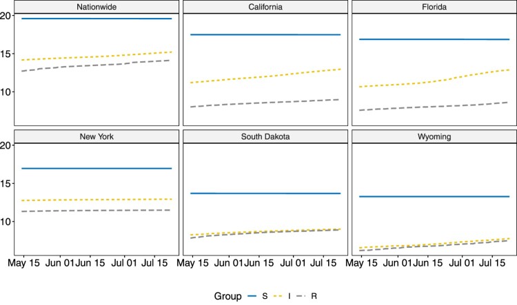
Note that the removal group for county-level data only contain deaths and there is no information available for recoveries. Similar to in Sun et al. [21], a three-point moving average filter is applied to the infectious group  $I\left(t\right)$ and removal group  $R\left(t\right)$ to reduce noise. Due to the large size of the susceptible group, the group sizes are visualized on a natural log scale in Figure 1 and Figure 2. The infectious and removal numbers are much smaller in SD and WY when compared to other states. As during the studied period, NY is still under lock-down, both the infectious and removal groups experienced slow increases. For CA and FL, however, potentially due to re-open in early May, their infectious and removal groups saw rapid increases. The three counties selected are the metropolitan areas in CA, FL and NY, and the trends observed are similar to those in their respective states.

Figure 1.

Visualizations for $S\left(t\right)$, $I\left(t\right)$ and $R\left(t\right)$ in US nationwide and five individual states on natural log scale.

Figure 2.

Visualizations for  $S\left(t\right)$, $I\left(t\right)$ and  $R\left(t\right)$ in the three selected counties on natural log scale.

3. Method

3.1. The SIR and vSIR models

In the SIR model, we consider a fixed total population of size N. By ‘fixed’, we assume that the population size does not vary over time. The effect of natural death or birth are not considered here, as the outstanding period of an infectious disease is much shorter than human average lifetime. Denote, at time t ( $t\ge 1$), the counts of susceptible, infectious, and recovered/removed persons within a given region as  $S\left(t\right)$,  $I\left(t\right)$ and  $R\left(t\right)$, respectively, and the relationship $N=S\left(t\right)+I\left(t\right)+R\left(t\right)$ always holds.

Two parameters in the SIR model are time-invariant: the transmission rate β, and the recovering rate γ. The transmission rate β controls how much the disease can be transmitted through exposure. It is jointly determined by the chance of contact and the probability of disease transmission. The recovering rate γ stands for the rate at which infected individuals recover or die. Time-varying property of these two parameters is ignored in traditional SIR modeling, which is a rather strong simplifying assumption that hurdles the model's prediction power for disease trend. Therefore, we adopt the time-varying SIR [vSIR; 3] framework, where both β and γ are functions of time t.

The vSIR model can be viewed as both a deterministic model and a stochastic model. The deterministic vSIR model allows us to describe the number of people in each compartment with the ordinary differential equations (ODEs). A generalized version of the deterministic vSIR model having infectious rate  $\mathrm{\text{β}}\left(t\right)$ and removal rate  $\gamma \left(t\right)$ with respect to time can be described as follows:

$$\begin{array}{rl}\frac{\mathrm{d}\mathrm{S}\left(\mathrm{t}\right)}{\mathrm{d}\mathrm{t}}& =\frac{-\mathrm{\text{β}}\left(t\right)I\left(t\right)S\left(t\right)}{N},\\ \frac{\mathrm{d}\mathrm{I}\left(\mathrm{t}\right)}{\mathrm{d}\mathrm{t}}& =\frac{\mathrm{\text{β}}\left(t\right)I\left(t\right)S\left(t\right)}{N}-\gamma \left(t\right)I\left(t\right),\\ \frac{\mathrm{d}\mathrm{R}\left(\mathrm{t}\right)}{\mathrm{d}\mathrm{t}}& =\gamma \left(t\right)I\left(t\right).\end{array}$$ (1)

While the deterministic vSIR model seems appealing due to its simplicity, the spread of a disease, however, is naturally stochastic. Disease transmission between two individuals is random rather than deterministic. The stochastic formulation of the vSIR model is, therefore, preferred for epidemic modeling purposes, as it allows for randomness in the disease spreading process.

3.2. Time fusion SIR model

Consider the the vSIR-Poisson process framework of Sun et al. [21] with two time-varying parameters, $\mathrm{\text{β}}\left(t\right)$ and  $\gamma \left(t\right)$. Let N be the total population, $M\left(t\right)=I\left(t\right)+R\left(t\right)$ denote the cumulative number of diagnosed cases and  $\mathrm{\Delta }M\left(t\right)=M\left(t\right)-M(t-1)$, $\mathrm{\Delta }R\left(t\right)=R\left(t\right)-R(t-1)$ represent the daily changes of  $M\left(t\right)$ and  $R\left(t\right)$. The initial values $\mathrm{\Delta }M\left(1\right)$ and $\mathrm{\Delta }R\left(1\right)$ are defaulted, respectively, to  $M\left(1\right)$ and $R\left(1\right)$. Let $t=1,\dots ,T$ denote the time domain. Hence we have

$$\begin{array}{rl}\mathrm{\Delta }M\left(t\right)& \sim \mathrm{P}\mathrm{o}\mathrm{i}\mathrm{s}\mathrm{s}\mathrm{o}\mathrm{n}\left(\frac{\mathrm{\text{β}}\left(t\right)S\left(t\right)I\left(t\right)}{N}\right),\\ \mathrm{\Delta }R\left(t\right)& \sim \mathrm{P}\mathrm{o}\mathrm{i}\mathrm{s}\mathrm{s}\mathrm{o}\mathrm{n}\left(\gamma \left(t\right)I\left(t\right)\right),t=2,\dots ,T.\end{array}$$ (2)

For most infectious diseases, the infectious and removal rates  $\mathrm{\text{β}}\left(t\right)$ and  $\gamma \left(t\right)$ do not always change smoothly over time, as they can be influenced by certain government policies in a notable manner. In other words, $\mathrm{\text{β}}\left(t\right)$ and  $\gamma \left(t\right)$ can fluctuate around a fixed value within a specific time period, and then with the inception of a policy, fluctuate around another value in a period that follows. Identifying the subpopulation structure of these two parameters with time fusion patterns in the SIR model will enhance our understanding of infectious diseases such as COVID-19. In this paper, we assume that successive differences of the infectious rate $\mathrm{\Delta }\mathrm{\text{β}}\left(t\right)=\mathrm{\text{β}}\left(t\right)-\mathrm{\text{β}}(t-1)$ and removal rate $\mathrm{\Delta }\gamma \left(t\right)=\gamma \left(t\right)-\gamma (t-1)$ both have an unknown clustered pattern with respect to time. Both  $\mathrm{\Delta }\mathrm{\text{β}}\left(1\right)$ and  $\mathrm{\Delta }\gamma \left(1\right)$ are defaulted to 0. For example, with a cluster of 0's in the successive differences, $\mathrm{\text{β}}\left(t\right)$ would remain constant over the corresponding time period. Toward this end, we use three different shrinkage priors on both  $\mathrm{\Delta }\mathrm{\text{β}}\left(t\right)$ and $\mathrm{\Delta }\gamma \left(t\right)$ to detect such clusters, including the student-t prior, horseshoe prior and spike-and-slab prior [see, 17,19 for more discussion]. As our proposed model focuses on time fusion, we name it hierarchical time fusion SIR (tf-SIR).

The first prior we consider is student-t prior. Despite the popularity of the Laplace prior, it has a light tail, suffers from posterior inconsistency issues [19,20], and often leads to smoothly varying estimation results, i.e. it cannot identify the clustered structure. The student-t prior, with its heavier tail, induces stronger shrinkage effect, and enjoys a nice posterior consistency property. The student-t shrinkage prior on the successive differences can be written as:

$$\begin{array}{rl}& \mathrm{\Delta }\mathrm{\text{β}}\left(t\right)\mid {\sigma }_{\mathrm{\text{β}}}^2\sim t_{d{f}_{\mathrm{\text{β}}}}\left(l_{\mathrm{\text{β}}}{\sigma }_{\mathrm{\text{β}}}\right),{\sigma }_{\mathrm{\text{β}}}^2\sim \mathrm{I}\mathrm{G}(a_{{\sigma }_{\mathrm{\text{β}}}},b_{{\sigma }_{\mathrm{\text{β}}}}),\mathrm{\text{β}}\left(1\right)\mid {\sigma }_{\mathrm{\text{β}}}^2\sim \mathrm{N}(0,{\sigma }_{\mathrm{\text{β}}}^2{\lambda }_1),\\ & \mathrm{\Delta }\gamma \left(t\right)\mid {\sigma }_{\gamma }^2\sim t_{d{f}_{\gamma }}\left(l_{\gamma }{\sigma }_{\gamma }\right),{\sigma }_{\gamma }^2\sim \mathrm{I}\mathrm{G}(a_{{\sigma }_{\gamma }},b_{{\sigma }_{\gamma }}),\gamma \left(1\right)\mid {\sigma }_{\gamma }^2\sim N(0,{\sigma }_{\gamma }^2{\eta }_1),t=2,\dots ,T,\end{array}$$

where T denotes the termination time of observation, $t_{{\omega }_1}\left({\omega }_2\right)$ denotes the student-t distribution with degree of freedom  ${\omega }_1$ and scale parameter  ${\omega }_2$, N() stands for the normal distribution, and IG() stands for the inverse gamma distribution. Note that the above student-t distribution can be rewritten as an inverse gamma scaled Gaussian mixture, and hence the tf-SIR model with student-t prior for the sequential differences in  $\mathrm{\text{β}}\left(t\right)$ and  $\gamma \left(t\right)$ can be alternatively formulated as:

$$\begin{array}{rl}& \mathrm{\Delta }\mathrm{\text{β}}\left(t\right)\mid {\sigma }_{\mathrm{\text{β}}}^2,{\lambda }_t\sim \mathrm{N}(0,{\lambda }_t{\sigma }_{\mathrm{\text{β}}}^2),{\lambda }_t\sim \mathrm{I}\mathrm{G}\left(a,b\right),\\ & \mathrm{\Delta }\gamma \left(t\right)\mid {\sigma }_{\gamma }^2,{\eta }_t\sim \mathrm{N}(0,{\eta }_t{\sigma }_{\gamma }^2),{\eta }_t\sim \mathrm{I}\mathrm{G}\left(c,d\right),\\ & {\sigma }_{\mathrm{\text{β}}}^2\sim \mathrm{I}\mathrm{G}\left(a_{{\sigma }_{\mathrm{\text{β}}}},b_{{\sigma }_{\mathrm{\text{β}}}}\right),{\sigma }_{\gamma }^2\sim \mathrm{I}\mathrm{G}\left(a_{{\sigma }_{\gamma }},b_{{\sigma }_{\gamma }}\right),t=2,\dots ,T,\end{array}$$ (3)

where a, b satisfy conditions $d{f}_{\mathrm{\text{β}}}=2a$ and $l_{\mathrm{\text{β}}}=\sqrt{\frac{b}{a}}$. Similarly, c, d satisfy conditions $d{f}_{\gamma }=2c$ and $l_{\gamma }=\sqrt{\frac{d}{c}}$. Both  ${\sigma }_{\mathrm{\text{β}}}^2$ and  ${\sigma }_{\gamma }^2$ are global parameters that shrink the successive differences toward 0. Following common practices, we assume inverse gamma priors for both to impart heavy tails, and keep the probability distribution further from 0 than the Gamma distribution. Different levels of sparsity can be achieved by varying the values of  ${\sigma }_{\mathrm{\text{β}}}^2$ and  ${\sigma }_{\gamma }^2$, with smaller values inducing stronger shrinkage toward 0.

The second prior is the horseshoe prior [2,3], which is a continuous shrinkage prior, and is one of the so called global-local shrinkage prior. It has exhibited ideal theoretical characteristics, and demonstrated good empirical performance [5,24]. Our tf-SIR model with the horseshoe prior can be expressed as:

$$\begin{array}{rl}& \mathrm{\Delta }\mathrm{\text{β}}\left(t\right)\mid {\sigma }_{\mathrm{\text{β}}}^2,{\lambda }_t\sim \mathrm{N}(0,{\lambda }_t^2{\sigma }_{\mathrm{\text{β}}}^2),{\lambda }_t\sim {\mathrm{C}}^{+}\left(0,1\right),\mathrm{\text{β}}\left(1\right)\mid {\sigma }_{\mathrm{\text{β}}}^2\sim \mathrm{N}(0,{\sigma }_{\mathrm{\text{β}}}^2{\lambda }_1),\\ & \mathrm{\Delta }\gamma \left(t\right)\mid {\sigma }_{\gamma }^2,{\eta }_t\sim \mathrm{N}(0,{\eta }_t^2{\sigma }_{\gamma }^2),{\eta }_t\sim {\mathrm{C}}^{+}\left(0,1\right),\gamma \left(1\right)\mid {\sigma }_{\gamma }^2\sim \mathrm{N}(0,{\sigma }_{\gamma }^2{\eta }_1),\\ & {\sigma }_{\mathrm{\text{β}}}^2\sim \mathrm{I}\mathrm{G}\left(a_{{\sigma }_{\mathrm{\text{β}}}},b_{{\sigma }_{\mathrm{\text{β}}}}\right),{\sigma }_{\gamma }^2\sim \mathrm{I}\mathrm{G}\left(a_{{\sigma }_{\gamma }},b_{{\sigma }_{\gamma }}\right),t=2,\dots ,T,\end{array}$$ (4)

where ${\sigma }_{\mathrm{\text{β}}}^2$ and ${\sigma }_{\gamma }^2$ are same as defined above, and ${\lambda }_t$ and ${\eta }_t$ are both local parameters following the half-Cauchy distribution ${\mathrm{C}}^{+}(0,1)$ that allows, respectively, some $\mathrm{\Delta }\mathrm{\text{β}}\left(t\right)$ and $\mathrm{\Delta }\gamma \left(t\right)$ to escape from the shrinkage.

Finally, our third prior of choice is the spike-and-slab prior [7,15]. It is a two component discrete mixture prior. In this paper, we write it as a two-component mixture of Gaussian distributions, and the model is expressed as:

$$\begin{array}{rl}& \mathrm{\Delta }\mathrm{\text{β}}\left(t\right)\mid {\sigma }_{\mathrm{\text{β}}}^2,{\lambda }_t\sim {\lambda }_t\mathrm{N}(0,{\sigma }_{\mathrm{\text{β}}}^2)+(1-{\lambda }_t)\mathrm{N}(0,{ϵ}^2),\\ & {\lambda }_t\sim \mathrm{B}\mathrm{e}\mathrm{r}\left(p\right),\mathrm{\text{β}}\left(1\right)\mid {\sigma }_{\mathrm{\text{β}}}^2\sim \mathrm{N}(0,{\sigma }_{\mathrm{\text{β}}}^2{\lambda }_1),\\ & \mathrm{\Delta }\gamma \left(t\right)\mid {\sigma }_{\gamma }^2,{\eta }_t\sim {\eta }_t\mathrm{N}(0,{\sigma }_{\gamma }^2)+(1-{\eta }_t)\mathrm{N}(0,{ϵ}^2),\\ & {\eta }_t\sim \mathrm{B}\mathrm{e}\mathrm{r}\left(\pi \right),\gamma \left(1\right)\mid {\sigma }_{\gamma }^2\sim \mathrm{N}(0,{\sigma }_{\gamma }^2{\eta }_1),\\ & {\sigma }_{\mathrm{\text{β}}}^2\sim \mathrm{I}\mathrm{G}\left(a_{{\sigma }_{\mathrm{\text{β}}}},b_{{\sigma }_{\mathrm{\text{β}}}}\right),{\sigma }_{\gamma }^2\sim \mathrm{I}\mathrm{G}\left(a_{{\sigma }_{\gamma }},b_{{\sigma }_{\gamma }}\right),t=2,\dots ,T,\end{array}$$ (5)

where  $ϵ\ll {\sigma }_{\mathrm{\text{β}}}^2$ and $ϵ\ll {\sigma }_{\gamma }^2$, ${\lambda }_t$ and  ${\eta }_t$ are indicators that take values in  $\{0,1\}$, $\mathrm{B}\mathrm{e}\mathrm{r}\left(\right)$ denotes the Bernoulli distribution, and again ${\sigma }_{\mathrm{\text{β}}}^2$ and ${\sigma }_{\gamma }^2$ are same as defined above. In this paper, we fix the inclusion probabilities p and π. In some cases, ϵ is set to 0 so that the spike is taken to a point mass at the origin  ${\delta }_0$. This distribution can be sensitive to prior choices of the slab width or prior inclusion probability, and therefore we choose the normal distribution with a small variance centered at 0 as the spike.

4. Simulation

4.1. Simulation designs

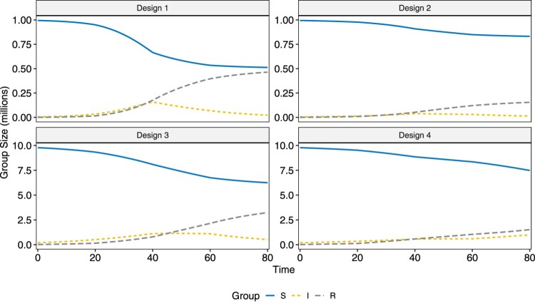
We use the R package SimInf [25] to generate data. Four designs over a time span of 80 days are considered. The time domain is divided into four equally sized pieces each spanning for 20 days, where both the infectious rate  $\mathrm{\text{β}}\left(t\right)$ and the removal rate  $\gamma \left(t\right)$ are piecewise constant within each of them. The four designs have different $\mathrm{\text{β}}\left(t\right)$, $\gamma \left(t\right)$, and population size N, and the numerical values are listed in Table 1. Four example datasets, one for each design, are visualized in Figure 3. Design 1 corresponds to a fairly high infectious disease with high removal/recovery rate and design 2 corresponds to a mildly infectious disease with similar removal/recovery rate. Designs 3 and 4 have larger population sizes, and a disease with smaller numerical values for  $\mathrm{\text{β}}\left(t\right)$ can infect a large portion of the population, such as demonstrated for Design 3. Design 4, with small  $\mathrm{\text{β}}\left(t\right)$ and  $\gamma \left(t\right)$, exhibits slow overall development. A total of 100 replicates are performed for each design. In each replicate, the length of the MCMC chain is set to 50,000. As the numerical values for  $\mathrm{\text{β}}\left(t\right)$ and  $\gamma \left(t\right)$ in all four designs are not large, it is essential that we get independent posterior samples. To ensure minimal correlation between draws, we set the thinning interval to 10 and set the burn-in to 3000, which leaves us 2000 samples to perform inference.

Table 1.

Parameters used in data generation under the four simulation settings.

Design	$\mathrm{\text{β}}\left(t\right)$ on pieces 1, 2, 3, 4	$\gamma \left(t\right)$ on pieces 1, 2, 3, 4	Population size
Design 1	(0.15, 0.20, 0.10, 0.05)	(0.05, 0.09, 0.10, 0.08)	${10}^6$
Design 2	(0.10, 0.15, 0.10, 0.05)	(0.05, 0.09, 0.10, 0.08)	${10}^6$
Design 3	(0.07, 0.09, 0.08, 0.05)	(0.02, 0.04, 0.06, 0.07)	${10}^7$
Design 4	(0.05, 0.08, 0.05, 0.07)	(0.02, 0.05, 0.04, 0.03)	${10}^7$

Figure 3.

Visualization of example datasets generated under each of the two simulation designs.

4.2. Performance measures

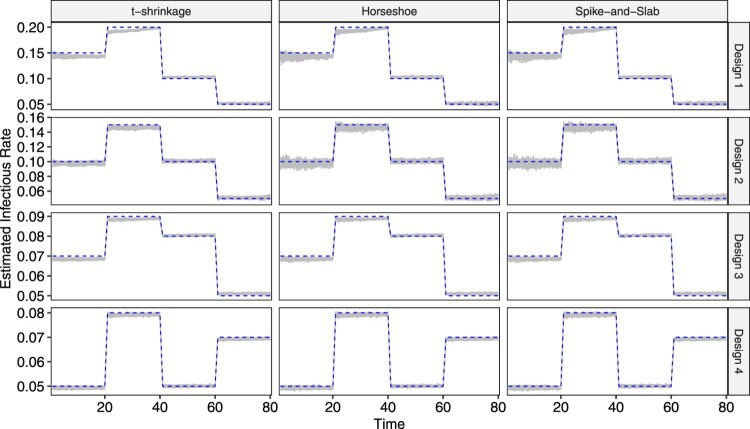
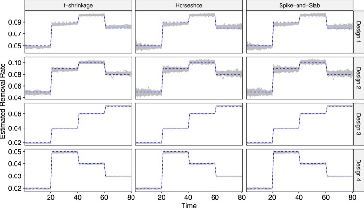
The parameter estimates for  $\mathrm{\text{β}}\left(t\right)$ and  $\gamma \left(t\right)$ for the 100 replicates are visualized respectively in Figures 4 and 5 as grey lines, and the true underlying values are also plotted in dashed lines. The first observation is that, under all four designs, all three models yield quite accurate parameter estimation performance, as the grey band formed by 100 parameters lie close to or around the dashed line in both plots. Secondly, as the population size in Design 3 and Design 4 is 10 times that in Design 1 and 2, their corresponding grey bands are, overall, tighter. Thirdly, in both figures, the grey bands corresponding to the t-shrinkage prior is narrower than those for horseshoe and spike-and-slab, indicating overall relatively stable estimation performance.

Figure 4.

Plot of estimated  $\mathrm{\text{β}}\left(t\right)$ in 100 replicates for each combination of design and prior. True values are overlaid in dashed lines.

Figure 5.

Plot of estimated  $\gamma \left(t\right)$ in 100 replicates for each combination of design and prior. True values are overlaid in dashed lines.

The estimation performance, in addition to visually, is also measured numerically. For  $\mathrm{\text{β}}\left(t\right)$, we apply the following three metrics:

$$\begin{array}{rl}{\mathrm{M}\mathrm{A}\mathrm{B}}_{\mathrm{\text{β}}}\left(t\right)& =\frac{1}{100}\sum _{\ell =1}^{100}\left|{\widehat{\mathrm{\text{β}}}}_{\ell }\left(t\right)-\mathrm{\text{β}}\left(t\right)\right|,\end{array}$$ (6)

$$\begin{array}{rl}{\mathrm{M}\mathrm{S}\mathrm{E}}_{\mathrm{\text{β}}}\left(t\right)& =\frac{1}{100}\sum _{\ell =1}^{100}{\left({\widehat{\mathrm{\text{β}}}}_{\ell }\left(t\right)-\mathrm{\text{β}}\left(t\right)\right)}^2,\end{array}$$ (7)

$$\begin{array}{rl}{\mathrm{S}\mathrm{D}}_{\mathrm{\text{β}}}\left(t\right)& =\frac{1}{99}\sum _{\ell =1}^{100}{\left({\widehat{\mathrm{\text{β}}}}_{\ell }\left(t\right)-\overline{\widehat{\mathrm{\text{β}}}}\left(t\right)\right)}^2,\end{array}$$ (8)

where ${\widehat{\mathrm{\text{β}}}}_{\ell }\left(t\right)$ is the posterior estimate of β at time t in the ℓth replicate for  $\ell =1,\dots ,100$ and  $t=1,\dots ,80$, and $\overline{\widehat{\mathrm{\text{β}}}}\left(t\right)=\frac{1}{100}\sum _{\ell =1}^{100}{\widehat{\mathrm{\text{β}}}}_{\ell }\left(t\right)$. The metrics for γ are defined in a similar manner, and therefore we omit the details.

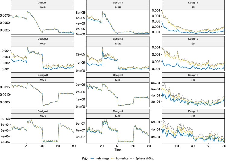
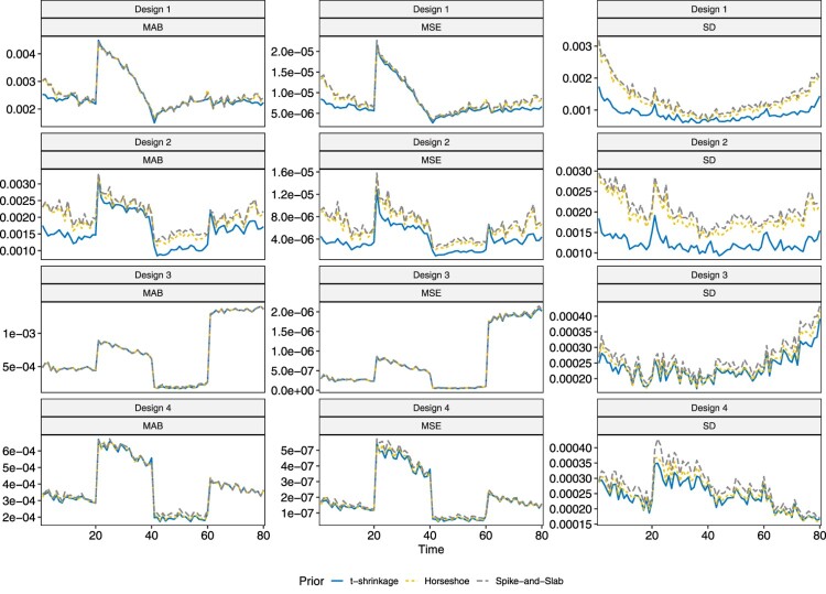
The three models are compared in terms of the three performance metrics in Figures 6 and 7. One interesting observation is that the MAB and MSE tend to be large near when $t\in \{20,40,60\}$, which corresponds to when changes in parameters occur. They then stabilize as the disease continues to develop. For relatively larger values of the true parameter, the MAB and MSE are larger than for small values of true parameters. As can be observed from the third column in both Figures 6 and 7, the horseshoe and spike-and-slab priors perform similarly in terms of MAB, MSE and SD. When the sample size is ${10}^6$, the t-shrinkage prior yields parameter estimates that are overall more stable and have smaller SD than the other two, which is consistent with the third observation for the grey bands. This difference, however, decreases with increase in sample size.

Figure 6.

Plot of MAB, MSE and SD of parameter estimate for  $\mathrm{\text{β}}\left(t\right)$ under different designs.

Figure 7.

Plot of MAB, MSE and SD of parameter estimate for  $\gamma \left(t\right)$ under different designs.

5. Real data analysis

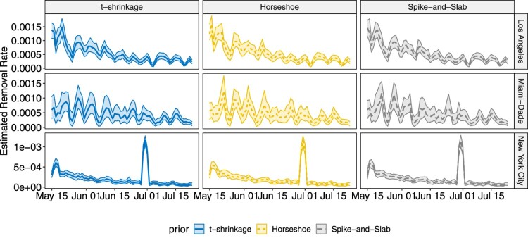
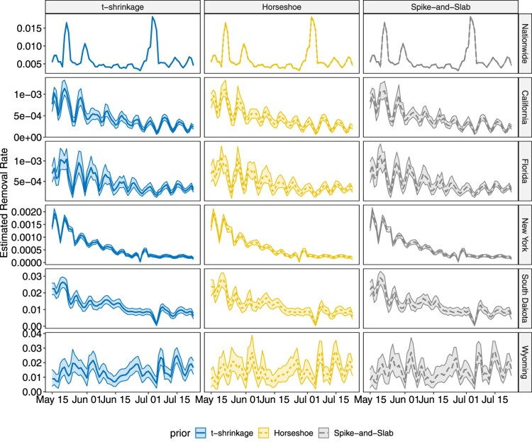
The proposed methodology is applied on COVID-19 data for both state-level and county level introduced in Section 2. Analysis for other states and counties can be conducted in the same way, which is omitted in this paper. Similar as the simulation studies, the chain length is set to 50,000 with thinning 10, and the first 3000 samples after thinning are treated as burn-in. The estimated infectious rates and removal rates, together with their 95% highest posterior density (HPD) intervals are shown in Figures 8 – 11.

Figure 10.

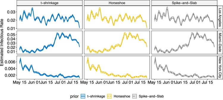
Plot for the estimated infectious rate  $\mathrm{\text{β}}\left(t\right)$ with 95% HPD intervals for the three selected counties over the studied time frame.

Figure 8.

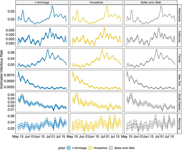
Plot for the estimated infectious rate  $\mathrm{\text{β}}\left(t\right)$ with 95% HPD intervals for US nationwide and five individual states over the studied time frame.

Figure 11.

Plot for the estimated removal rate  $\gamma \left(t\right)$ with 95% HPD intervals for the three selected counties over the studied time frame.

In both state-level and county-level, the three different priors yield similar results. From Figures 8 and 9, we find the infectious rate for NY is smaller than other states during this period. Also, the relatively stable $\widehat{\mathrm{\text{β}}}\left(t\right)$ for NY after June 6th indicates a potential cluster. FL witnesses a pump peak after mid June, which results from the aggressive reopen in FL. The clustered pattern in other states, however, is not as clear as that in NY, which is partially due to the fact that testing and reporting are conducted timely in NY as it is one of the initial hotspots in March and April that experienced high growth of COVID-19 cases, while in the other states that we considered, there is more delay in testing and reporting. As the number of cumulative cases and daily new cases are large in CA, FL and NY, the HPD band for $\widehat{\mathrm{\text{β}}}\left(t\right)$ is tight, while in SD and WY, where daily new cases do not exceed, respectively, 100 and 50, the estimated HPD band is much wider. As for the removal rate, NY, FL and CA have similar result. Despite the differences in numerical values, the trends of $\hat{\gamma }\left(t\right)$ for NY and FL are similar, and display a weekly seasonality, with the estimated removal rates being smaller than average on weekends. This is due to the fact that reporting is less active during weekends than during the week. Note that for SD, the estimated removal rate clearly shows a relatively stable pattern between June 20th and July 1st, indicating the existence of a potential cluster. The nation-wide removal rate estimate is constant across the time and has few peaks during this time period, as a few states release the recovered cases in a cumulative manner on a certain day. On the county level, $\widehat{\mathrm{\text{β}}}\left(t\right)$ for New York City becomes stable after June 15th. The infectious rate estimate for Miami-Dade remained relatively low before June 22nd but started to increase, and remained relatively high. For Los Angeles, $\widehat{\mathrm{\text{β}}}\left(t\right)$ experiences fluctuations with weekly seasonality, but the overall trend remains stable. The estimated removal rates are very small in all three counties, and all have wide HPD bands, since the removal group only contains deaths in county-level data. The sudden jump in Figure 11 for New York City corresponds to the release of 633 death cases, which was due to data anomaly.

Figure 9.

Plot for the estimated removal rate  $\gamma \left(t\right)$ with 95% HPD intervals for US nationwide and five individual states over the studied time frame.

6. Conclusion

In this paper, we proposed the tf-SIR model to capture group structure for infectious rate and removal rate of different time period by using Bayesian shrinkage priors. To our best knowledge, this is the first attempt in literature to use Bayesian shrinkage to recover unknown grouping structure for SIR model. Our simulation results indicate that the proposed method has reasonable performance and ability to capture the group pattern of infectious rate and removal rate. The analysis of COVID-19 data also brings in new understanding of the infectious disease such as COVID-19. Also, our tf-SIR model can not only be used to model and assess COVID-19 pandemic but also other epidemic.

One interesting consideration, as suggested by one anonymous reviewer, is to use a supermartingale structure, i.e. non-increasing function with respective to time, to model the infectious rate  $\mathrm{\text{β}}\left(t\right)$ because of the implementation of policy intervention. While such assumption might not be met by the development of COVID-19 in the United States, it is a quite reasonable assumption when studying the course of development for COVID-19 in countries where quarantine and stay-at-home policies are strictly enforced such as China, Singapore, and Vietnam.

In addition, three topics beyond the scope of this paper are worth further investigation. First, in our real data application, a moving average approach is applied to deal with measurement errors for observed data. Proposing a measurement error model with SIR is an interesting future work. Furthermore, different states may have similar infection and removal pattern. Subgroup detection for different states will help the government design its polices. Finally, discovering theoretical guarantees such as posterior concentration rates of proposed methods is also devoted to future research.

Disclosure statement

No potential conflict of interest was reported by the author(s).

References

- 1.Casella G., Ghosh M., Gill J., and Kyung M., Penalized regression, standard errors, and Bayesian lassos, Bayesian Anal. 5 (2010), pp. 369–411. [Google Scholar]
- 2.Carvalho C.M., Polson N.G., and Scott J.G., Handling Sparsity via the Horseshoe, in Proceedings of the Twelfth International Conference on Artificial Intelligence and Statistics, Vol. 5, D. van Dyk and M. Welling, eds., Proceedings of Machine Learning Research, pp. 16–18 Apr, Hilton Clearwater Beach Resort, Clearwater Beach, Florida, USA, PMLR, 2009, pp. 73–80.
- 3.Carvalho C.M., Polson N.G., and Scott J.G., The horseshoe estimator for sparse signals, Biometrika 97 (2010), pp. 465–480. [Google Scholar]
- 4.Chen Y.C., Lu P.E., Chang C.S. and Liu T.H., A time-dependent SIR model for COVID-19 with undetectable infected persons, IEEE Trans. Netw. Sci. Eng. 7 (2020), pp. 3279–3294. [DOI] [PMC free article] [PubMed] [Google Scholar]
- 5.Datta J. and Ghosh J.K., Asymptotic properties of Bayes risk for the horseshoe prior, Bayesian Anal. 8 (2013), pp. 111–132. [Google Scholar]
- 6.de Valpine P., Turek D., Paciorek C.J., Anderson-Bergman C., Lang D.T., and Bodik R., Programming with models: Writing statistical algorithms for general model structures with NIMBLE, J. Comput. Graph. Stat. 26 (2017), pp. 403–413. [Google Scholar]
- 7.George E.I. and McCulloch R.E., Variable selection via Gibbs sampling, J. Amer. Statist. Assoc. 88 (1993), pp. 881–889. [Google Scholar]
- 8.Guidotti E. and Ardia D., COVID-19 data hub, 2020, working paper. Available at https://covid19datahub.io.
- 9.Hethcote H.W., The mathematics of infectious diseases, SIAM Rev. 42 (2000), pp. 599–653. [Google Scholar]
- 10.Hu G. and Geng J., Heterogeneity learning for SIRS model: An application to the COVID-19, Stat. Interface 14 (2021), pp. 73–81. [Google Scholar]
- 11.Jung S.Y., Jo H., Son H., and Hwang H.J., Real-world implications of a rapidly responsive COVID-19 spread model with time-dependent parameters via deep learning: Model development and validation, J. Med. Internet. Res. 22 (2020), p. e19907. [DOI] [PMC free article] [PubMed] [Google Scholar]
- 12.Kermack W.O. and McKendrick A.G., A contribution to the mathematical theory of epidemics, Proc. R. Soc. Lond. Ser. A. 115 (1927), pp. 700–721. [Google Scholar]
- 13.Kermack W.O. and McKendrick A.G., Contributions to the mathematical theory of epidemics. II. The problem of endemicity, Proc. R. Soc. Lond. Ser. A 138 (1932), pp. 55–83. [Google Scholar]
- 14.Kermack W.O. and McKendrick A.G., Contributions to the mathematical theory of epidemics. III. Further studies of the problem of endemicity, Proc. R. Soc. Lond. Ser. A 141 (1933), pp. 94–122. [Google Scholar]
- 15.Mitchell T.J. and Beauchamp J.J., Bayesian variable selection in linear regression, J. Amer. Statist. Assoc. 83 (1988), pp. 1023–1032. [Google Scholar]
- 16.Park T. and Casella G., The Bayesian lasso, J. Amer. Statist. Assoc. 103 (2008), pp. 681–686. [Google Scholar]
- 17.Piironen J. and Vehtari A., Sparsity information and regularization in the horseshoe and other shrinkage priors, Electron. J. Stat. 11 (2017), pp. 5018–5051. [Google Scholar]
- 18.Read J.M., Bridgen J.R., Cummings D.A., Ho A., and Jewell C.P., Novel coronavirus 2019-nCoV: Early estimation of epidemiological parameters and epidemic predictions, MedRxiv (2020). doi: 10.1101/2020.01.23.20018549. [DOI] [PMC free article] [PubMed] [Google Scholar]
- 19.Song Q. and Cheng G., Bayesian fusion estimation via t shrinkage, Sankhya A (2019), pp. 1–33. [Google Scholar]
- 20.Song Q. and Liang F., Nearly optimal Bayesian shrinkage for high dimensional regression, arXiv preprint arXiv:1712.08964 (2017).
- 21.Sun H., Qiu Y., Yan H., Huang Y., Zhu Y., and Chen S.X., Tracking reproductivity of COVID-19 epidemic in China with varying coefficient SIR model, J. Data Sci. 18 (2020), pp. 455–472. [Google Scholar]
- 22.Tang B., Wang X., Li Q., Bragazzi N.L., Tang S., Xiao Y., and Wu J., Estimation of the transmission risk of the 2019-nCoV and its implication for public health interventions, J. Clin. Med. 9 (2020), pp. 462. [DOI] [PMC free article] [PubMed] [Google Scholar]
- 23.Tibshirani R., Saunders M., Rosset S., Zhu J., and Knight K., Sparsity and smoothness via the fused lasso, J. R. Stat. Soc. Ser. B. (Stat. Methodol.) 67 (2005), pp. 91–108. [Google Scholar]
- 24.Van Der Pas S.L., Kleijn B.J., and Van Der Vaart A.W., The horseshoe estimator: Posterior concentration around nearly black vectors, Electron. J. Stat. 8 (2014), pp. 2585–2618. [Google Scholar]
- 25.Widgren S., Bauer P., Eriksson R., and Engblom S., SimInf: An R package for data-driven stochastic disease spread simulations, J. Stat. Softw. 91 (2019), pp. 1–42. [Google Scholar]
- 26.World Health Organization , WHO coronavirus disease (COVID-19) dashboard, 2020. Available at https://covid19.who.int/ (accessed 20 July 2020).
- 27.Wu J.T., Leung K., and Leung G.M., Nowcasting and forecasting the potential domestic and international spread of the 2019-nCoV outbreak originating in Wuhan, China: A modelling study, Lancet 395 (2020), pp. 689–697. [DOI] [PMC free article] [PubMed] [Google Scholar]
Associated Data
This section collects any data citations, data availability statements, or supplementary materials included in this article.