Differentially Private Bayesian Neural Networks on Accuracy, Privacy and Reliability

Abstract

Bayesian neural network (BNN) allows for uncertainty quantification in prediction, offering an advantage over regular neural networks that has not been explored in the differential privacy (DP) framework. We fill this important gap by leveraging recent development in Bayesian deep learning and privacy accounting to offer a more precise analysis of the trade-off between privacy and accuracy in BNN. We propose three DP-BNNs that characterize the weight uncertainty for the same network architecture in distinct ways, namely DP-SGLD (via the noisy gradient method), DP-BBP (via changing the parameters of interest) and DP-MC Dropout (via the model architecture). Interestingly, we show a new equivalence between DP-SGD and DP-SGLD, implying that some non-Bayesian DP training naturally allows for uncertainty quantification. However, the hyperparameters such as learning rate and batch size, can have different or even opposite effects in DP-SGD and DP-SGLD. Extensive experiments are conducted to compare DP-BNNs, in terms of privacy guarantee, prediction accuracy, uncertainty quantification, calibration, computation speed, and generalizability to network architecture. As a result, we observe a new tradeoff between the privacy and the reliability. When compared to non-DP and non-Bayesian approaches, DP-SGLD is remarkably accurate under strong privacy guarantee, demonstrating the great potential of DP-BNN in real-world tasks.

1. Introduction

Deep learning has exhibited impressively strong performance in a wide range of classification and regression tasks. However, standard deep neural networks do not capture the model uncertainty and fail to provide the information available in statistical inference, which is crucial to many applications where poor decisions are accompanied with high risks. As a consequence, neural networks are prone to overfitting and being overconfident about their prediction, reducing their generalization capability and more importantly, their reliability. From this perspective, Bayesian neural network (BNN) [22,23,7,27] is highly desirable and useful as it characterizes the model’s uncertainty, which on one hand offers a reliable and calibrated prediction interval that indicates the model’s confidence [35,15,4,19], and on the other hand reduces the prediction error through the model averaging over multiple weights sampled from the learned posterior distribution. For example, networks with the dropout [31] can be viewed as a Bayesian neural network by [13]; the dropout improves the accuracy from 57% [37] to 63% [31] on CIFAR100 image dataset and 69.0% to 70.4% on Reuters RCV1 text dataset [31]. In another example, on a genetics dataset where the task is to predict the occurrence probability of three alternative-splicing-related events based on RNA features. The performance of ‘Code Quality’ (a measure of the KL divergence between the target and the predicted probability distributions) can be improved from 440 on standard network to 623 on BNN [36].

In a long line of research, much effort has been devoted to making BNNs accurate and scalable. These approaches can be categorized into three main classes: (i) by introducing random noise into gradient methods (e.g. SG-MCMC [34]) to quantify the weight uncertainty; (ii) by considering each weight as a distribution, instead of a point estimate, so that the uncertainty is described inside the distribution; (iii) by introducing randomness on the network architecture (e.g. the dropout) that leads to a stochastic training process whose variability characterizes the model’s uncertainty. To be more specific, we will discuss these methods including the Stochastic Gradient Langevin Descent (SGLD) [21], the Bayes By Backprop (BBP) [4] and the Monte Carlo Dropout (MC Dropout) [13].

Another natural yet urgent concern on the standard neural networks is the privacy risk. The use of sensitive datasets that contain information from individuals, including medical records, email contents, financial statements, and photos, has incurred serious risk of privacy violation. For example, the sale of Facebook user data to Cambridge Analytica [8] leads to the $5 billion fine to the Federal Trade Commission for its privacy leakage. As a gold standard to protect the privacy, the differential privacy (DP) has been introduced by [11] and widely applied to deep learning [1,5,30,6], due to its mathematical rigor.

Although both uncertainty quantification and privacy guarantee have drawn increasing attention, most existing work studied these two perspectives separately. Previous arts either studied DP Bayesian linear models [34,38] or studied DP-BNN using SGLD [20] but only for the accuracy measure without uncertainty quantification. In short, to the best of our knowledge, no existing deep learning models have equipped with the differential privacy and the Bayesian uncertainty quantification simultaneously.

Our proposal contributes on several fronts. First, We propose three distinct DP-BNNs that all use the DP-SGD (stochastic gradient descent) but characterize the weight uncertainty in fundamentally distinct ways, namely DP-SGLD (via the noisy gradient method), DP-BBP (via changing the parameters of interest), and DP-MC Dropout (via the model architecture). Our DP-BNNs are essentially DP Bayesian training procedures, as summarized in Figure 10, while the inference procedures of DP-BNNs are the same as regular non-private BNNs.

Second, we establish the precise connection between the Bayesian gradient method, DP-SGLD and the non-Bayesian method, DP-SGD. Through a rigorous analysis, we show that DP-SGLD is a sub-class of DP-SGD yet the training hyperparameters (e.g. learning rate and batch size) have very different impacts on the performance of these two methods.

Finally, We empirically evaluate DP-BNNs through the classification and regression tasks. Notice that although all three DP-BNNs are equally private and capable of uncertainty quantification, their performance can be significantly different under various measures, as discussed in Section 4.

2. Differentially Private Neural Networks

In this work, we consider (ϵ, δ)-DP and also use μ-GDP as a tool to compose the privacy loss ϵ iteratively. We first introduce the definition of (ϵ, δ)-DP in [12].

Definition 1. A randomized algorithm M is (ε, δ)-differentially private (DP) if for any pair of datasets S, S′ that differ in a single sample, and any event E,

$$\mathbb{P}\left[M\left(S\right)\in E\right]⩽{\text{e}}^{\epsilon }\mathbb{P}\left[M\left(S^{\prime }\right)\in E\right]+\delta .$$ (1)

A common approach to learn a DP neural network (NN) is to use DP gradient methods, such as DP-SGD (see Algorithm 1; possibly with the momentum and weight decay) and DP-Adam [5], to update the neural network parameters, i.e. weights and biases. In order to guarantee the privacy, DP gradient methods differ from its non-private counterparts in two steps. For one, the gradients are clipped on a per-sample basis, by a pre-defined clipping norm C. This is to ensure the sum of gradients has a bounded sensitivity to data points (this concept is to be defined in Appendix A). We note that in non-neural-network training, DP gradient methods may apply without the clipping, for instance, DP-SGLD in [34] requires no clipping and is thus different from our DP-SGLD in Algorithm 2 (also our DP-SGLD need not to modify the noise scale). For the other, some level of random Gaussian noises are added to the clipped gradient at each iteration. This is known as the Gaussian mechanism which has been rigorously shown to be DP by [12, Theorem 3.22].

$$\begin{array}{l}\overline{\underset{¯}{\mathbf{Algorithm\; 1:}\text{ Differentially private SGD (DP-SGD) with regularization\hspace{0.17em}\hspace{0.17em}\hspace{0.17em}\hspace{0.17em}\hspace{0.17em}\hspace{0.17em}\hspace{0.17em}\hspace{0.17em}\hspace{0.17em}\hspace{0.17em}\hspace{0.17em}}}}\\ \mathbf{Input:}\text{ Examples }\left\{\left({\mathit{\text{x}}}_i,y_i\right)\right\},\text{\hspace{0.17em}loss\hspace{0.17em}}𝓁\left(\cdot ;\mathit{w}\right),\text{\hspace{0.17em}regularization\hspace{0.17em}}r\left(\mathit{w}\right).\\ \mathbf{for}t=1toT\mathbf{do}\\ \text{\hspace{1em}\hspace{1em}Randomly\hspace{0.17em}sample\hspace{0.17em}}{B}_t\subset \left\{1,2,\dots ,N\right\};\\ \mathbf{for}i\in B_t\mathbf{do}\\ \text{\hspace{1em}\hspace{1em}\hspace{1em}Compute\hspace{0.17em}}{g}_i={\nabla }_{\mathit{w}}𝓁\left(x_i,y_i;{\mathit{w}}_{t-1}\right)\\ \text{\hspace{1em}\hspace{1em}\hspace{1em}Clip\hspace{0.17em}}{\tilde{g}}_i=\min \left\{1,\frac{C_t}{{‖g_i‖}_2}\right\}\cdot g_i.;\\ \text{\hspace{1em}\hspace{1em}Add\hspace{0.17em}noise\hspace{0.17em}}\widehat{g}=\frac{1}{\left|B_t\right|}{\sum }_{i\in B_t}{\tilde{g}}_i+\frac{\sigma \cdot C_t}{\left|B_t\right|}\cdot 𝒩\left(0,I_d\right).\\ \text{\hspace{1em}\hspace{1em}Update\hspace{0.17em}}{\mathit{w}}_t\leftarrow {\mathit{w}}_{t-1}-{\eta }_t\left(\widehat{g}+{\nabla }_{\mathit{w}}r\left({\mathit{w}}_{t-1}\right)\right);\\ \underset{¯}{\mathbf{Output:}{\mathit{w}}_1,{\mathit{w}}_2,\cdots ,{\mathit{w}}_T}\end{array}$$

In the training of neural networks, the Gaussian mechanism is applied multiple times and the privacy loss ϵ accumulates, indicating the model becomes increasingly vulnerable to privacy risk though more accurate. To compute the total privacy loss, we leverage the recent privacy accounting methods: Gaussian differential privacy (GDP) [10,5] and Moments accountant [1,9]. Both methods give valid though different upper bounds of ϵ as a consequence of using different composition theories. Notably, the rate at which the privacy compromises depends on the certain hyperparameters, such as the number of iterations T, the learning rate η, the noise scale σ, the batch size |B|, the clipping norm C. In the following sections, we exploit how these training hyperparameters influences DP and the convergence, and subsequently the uncertainty quantification.

3. Bayesian Neural Networks

BNNs have achieved significant success recently, by incorporating expert knowledge and making statistical inference through uncertainty quantification. On the high level, BNNs share the same architecture as regular NNs f (x; w) but are different in that BNNs treat weights as a probability distribution instead of a single deterministic value. Learned properly, these weight distributions can characterize the uncertainty in prediction and improve the generalization behavior. For example, suppose we have obtained the weight distribution W, then the prediction distribution of BNNs is f(x;W), which is unavailable by regular NNs. We now describe three popular yet distinct approaches to learn BNNs, leaving the algorithms in Section 4, which has the DP-BNNs but reduces to non-DP BNNs when σ = 0 (no noise) and C_t = ∞ (no clipping). We highlight that all three approaches are heavily based on SGD (though other optimizers can also be used): the difference lies in how SGD is applied. The Pytorch implementation is available at github.com/JavierAntoran/Bayesian-Neural-Networks.

3.1. Bayesian Neural Networks via Sampling

Stochastic Gradient Langevin Dynamics (SGLD)

SGLD [35,21] is a gradient method that applies on the weights w of NN, and the weight uncertainty arises from the random noises injected into the training dynamics. Therefore, SGLD works on regular NN without any modification. However, unlike SGD, SGLD makes w to converge to a posterior distribution rather than to a point estimate, from which SGLD can sample and characterize the uncertainty of w. In details, SGLD takes the following form

$${\mathit{w}}_t={\mathit{w}}_{t-1}+{\eta }_t\left(\nabla \log p\left({\mathit{w}}_{t-1}\right)+\frac{n}{\left|B_t\right|}{\sum }_{i\in B_t}\nabla \log p\left({\mathit{\text{x}}}_i,y_i|{\mathit{w}}_{t-1}\right)\right)+𝒩\left(0,{\eta }_t\right)$$

where p(w) is the pre-defined prior distribution of weights and p(x, y|w) is the likelihood of data. In the literature of empirical risk minimization, SGLD can be viewed as SGD with random Gaussian noise in the updates:

$${\mathit{w}}_t={\mathit{w}}_{t-1}+{\eta }_t\left(\nabla r\left({\mathit{w}}_{t-1}\right)+\frac{n}{\left|B_t\right|}{\sum }_{i\in B_t}\nabla 𝓁\left({\mathit{\text{x}}}_i,y_i;{\mathit{w}}_{t-1}\right)\right)+𝒩\left(0,{\eta }_t\right),$$

where r(w) is the regularization and ℓ(x, y;w) is loss. We summarize in Footnote 1 an one-to-one correspondence between the regularization r(w) and the prior p(w), as well as between the loss ℓ(x, y;w) and the likelihood p(x, y|w). Writing the penalized loss as ${ℒ}_{\text{SGLD}}\left({\mathit{\text{x}}}_i,y_i;\mathit{w}\right):=n\cdot 𝓁\left({\mathit{\text{x}}}_i,y_i;\mathit{w}\right)+r\left(\mathit{w}\right)$, we obtain

$${\mathit{w}}_t={\mathit{w}}_{t-1}-\frac{{\eta }_t}{\left|B_t\right|}{\sum }_{i\in B_t}\frac{\partial {ℒ}_{\text{SGLD}}\left({\mathit{\text{x}}}_i,y_i;{\mathit{w}}_{t-1}\right)}{\partial {\mathit{w}}_{t-1}}+𝒩\left(0,{\eta }_t\right).$$

Interestingly, although SGLD adds an isotropic Gaussian noise to the gradient (similar to DP-SGD in Algorithm 1), it is not guaranteed as DP without the per-sample gradient clipping. Nevertheless, while SGLD is different from SGD, we show in Theorem 1 that DP-SGLD is indeed a sub-class of DP-SGD.

3.2. Bayesian Neural Networks via Optimization

In contrast to SGLD, which is considered as a sampling approach that modifies the updating algorithm, we now introduce two optimization approaches of BNNs that use the regular optimizers like SGD, but modify the objective of minimization or the network architecture instead.

Bayes By Backprop (BBP)

BBP [4] uses the standard SGD except it is applied on the hyperparameters of of pre-defined weight distributions, rather than on the weights w directly. For example, suppose we assume that $w~𝒩\left(\mu ,{\sigma }^2\right)$. Then BBP updates hyperparameters (μ, σ) while the regular SGD updates w.

This approach is known as the ‘variational inference’ or the ‘variational Bayes’, where a variational distribution q(w|θ) is learned through its governing hyperparameter θ. Consequently, the weight uncertainty is included in such variational distribution from which we can sample during the inference time.

In order to update the hyperparameter θ, the objective of minimization requires highly non-trivial transformation from $𝓁\left(\mathit{x},y;w\right)$ and is derived as follows. Given data D = {(x_i, y_i)}, the likelihood is $p\left(D|w\right)={\Pi }_{i}p\left(y_i|{\mathit{\text{x}}}_i,\mathit{w}\right)$ under some probabilistic model p(y|x,w). By the Bayes theorem, the posterior distribution p(w|D) is proportional to the likelihood and the prior distribution p(w),

$$p\left(w|D\right)\propto p\left(D|w\right)p\left(w\right)={\Pi }_{i}p\left(y_i|x_i,w\right)p\left(w\right).$$

Within a pre-specified variational distribution q(w|θ), we seek the distributional parameter θ such that q(w|θ) ≈ p(w|D). Conventionally, the variational distribution is restricted to be Gaussian and we learn its mean and standard deviation θ = (μ, σ) through minimizing the KL divergence:

$${\min }_{\theta }KL\left(q\left(w|\theta \right)\left|\right|p\left(w|D\right)\right)\equiv \mathbb{E}\log q\left(w|\theta \right)-\mathbb{E}\log p\left(w\right)-\mathbb{E}\log p\left(D|w\right).$$ (2)

This objective function is analytically intractable but can be approximated by drawing w^(j) from q(w|θ) for N independent times:

$${ℒ}_{\text{BBP}}\left(D;\theta \right):=\frac{1}{N}{\sum }_{j\in \left[N\right]}\log q\left(w^{\left(j\right)}|\theta \right)+r\left(w^{\left(j\right)}\right)+𝓁\left(D;{\mathit{w}}^{\left(j\right)}\right)$$

This approximated KL divergence is the actual objective to optimize instead of $𝓁\left(D;w\right)$ used by the non-Bayesian NN (see the derivation of ${ℒ}_{\text{BBP}}$ in Appendix B.1). It follows that in BBP, the SGD updating rule for the reparameterization θ = (μ, ρ) with σ = log(1 + exp(ρ)) is

$${\mu }_t={\mu }_{t-1}-\frac{{\eta }_t}{\left|B_t\right|}{\sum }_{i\in B_t}\frac{d{ℒ}_{\text{BBP}}\left({\mathit{\text{x}}}_i,y_i\right)}{d\mu },{\rho }_t={\rho }_{t-1}-\frac{{\eta }_t}{\left|B_t\right|}{\sum }_{i\in B_t}\frac{d{ℒ}_{\text{BBP}}\left({\mathit{\text{x}}}_i,y_i\right)}{d\rho }.$$

Monte Carlo Dropout (MC Dropout)

MC Dropout is proposed by [13] that establishes an interesting connection: optimizing the loss with L₂ penalty in regular NNs with dropout layers is equivalent to learning Bayesian inference approximately. From this perspective, the weight uncertainty is described by the randomness of the dropout operation. We refer to Appendix B.2 for an in-depth review of MC dropout.

In more details, denoting ${ℒ}_{\text{Dropout}}\left({\mathit{\text{x}}}_i,y_i;\mathit{w}\right):=𝓁\left({\mathit{\text{x}}}_i,y_i;\mathit{w}\right)+r\left(\mathit{w}\right)$, such connection claims equivalence between the problem ${\min }_{\mathit{w}}\frac{1}{n}{\sum }_{i=1}^n{ℒ}_{\text{Dropout}}\left({\mathit{\text{x}}}_i,y_i;\mathit{w}\right)$ and the variational inference problem (2), when the prior distribution is a zero mean Gaussian one. This equivalence makes MC Dropout similar to BBP in the sense of minimizing the same KL divergence. Nevertheless, while BBP directly minimizes the KL divergence, MC Dropout in practice leverages the equivalence to minimize the regular loss $𝓁\left(D;w\right)$ via the empirical risk minimization. Hence MC Dropout also shares similarity with SGD or SGLD. From the algorithmic perspective, suppose w_t is the remaining weights after the dropout in the t-th iteration, then the updating rule for MC Dropout with SGD is

$${\mathit{w}}_t={\mathit{w}}_{t-1}-\frac{{\eta }_t}{\left|B_t\right|}{\sum }_{i\in B_t}\frac{\partial {ℒ}_{\text{Dropout}}\left({\mathit{\text{x}}}_i,y_i;{\mathit{w}}_{t-1}\right)}{\partial {\mathit{w}}_{t-1}}.$$

4. Differentially Private Bayesian Neural Networks

To prepare the development of DP-BNNs, we summarize how to transform a regular NN to be Bayesian and to be DP, respectively. To learn a BNN, we need to establish the relationship between the Bayesian quantities (likelihood and prior) and the optimization loss and regularization. Under the Bayesian regime, $𝓁$ is the negative log-likelihood – log p(x, y|θ) and log p(θ) is the log-prior. Under the empirical risk minimization regime, $𝓁$ is the loss function and we view – log p(θ) as the regularization or penalty¹. To learn a DP network, we simply apply DP gradient methods that guarantee DP via the Gaussian mechanism (see Appendix A). Therefore, we can privatize each BNN to gain DP guarantee by applying DP gradient methods to update the parameters, as shown in Figure 10 and Figure 11 in Appendix E.

Although the high-level ideas of DP-BNNs are easy to understand, we emphasize that different DP-BNNs vary significantly in terms of generalizability, computation efficiency, and uncertainty quantification (see Table 5).

4.1. Differentially Private Stochastic Gradient Langevin Dynamics

$$\begin{array}{l}\overline{\underset{¯}{\mathbf{Algorithm\; 2:}\text{ Differentially private SGLD (DP-SGLD)\hspace{0.17em}\hspace{0.17em}\hspace{0.17em}\hspace{0.17em}\hspace{0.17em}\hspace{0.17em}\hspace{0.17em}\hspace{0.17em}\hspace{0.17em}\hspace{0.17em}\hspace{0.17em}\hspace{0.17em}\hspace{0.17em}\hspace{0.17em}\hspace{0.17em}\hspace{0.17em}\hspace{0.17em}\hspace{0.17em}\hspace{0.17em}\hspace{0.17em}\hspace{0.17em}\hspace{0.17em}\hspace{0.17em}\hspace{0.17em}\hspace{0.17em}\hspace{0.17em}\hspace{0.17em}\hspace{0.17em}\hspace{0.17em}\hspace{0.17em}\hspace{0.17em}\hspace{0.17em}\hspace{0.17em}\hspace{0.17em}\hspace{0.17em}\hspace{0.17em}\hspace{0.17em}\hspace{0.17em}\hspace{0.17em}\hspace{0.17em}\hspace{0.17em}\hspace{0.17em}\hspace{0.17em}\hspace{0.17em}\hspace{0.17em}\hspace{0.17em}\hspace{0.17em}\hspace{0.17em}\hspace{0.17em}}}}\\ \mathbf{Input:}\text{ Examples }\left\{\left({\mathit{\text{x}}}_i,y_i\right)\right\},\text{\hspace{0.17em}loss\hspace{0.17em}}𝓁\left(\cdot ;\mathit{w}\right),\text{\hspace{0.17em}regularization\hspace{0.17em}}r\left(\mathit{w}\right).\\ \mathbf{for}t=1toT\mathbf{do}\\ \text{\hspace{1em}\hspace{1em}Randomly\hspace{0.17em}sample\hspace{0.17em}a\hspace{0.17em}batch\hspace{0.17em}}{B}_t\subset \left\{1,2,\dots ,n\right\};\\ \mathbf{for}i\in B_t\mathbf{do}\\ \text{\hspace{1em}\hspace{1em}\hspace{1em}Compute\hspace{0.17em}}{g}_i={\nabla }_{\mathit{w}}𝓁\left(x_i,y_i;{\mathit{w}}_{t-1}\right)\\ \text{\hspace{1em}\hspace{1em}\hspace{1em}Clip\hspace{0.17em}}{\tilde{g}}_i=\min \left\{1,\frac{C_t}{{‖g_i‖}_2}\right\}\cdot g_i.;\\ \text{\hspace{1em}\hspace{1em}Update\hspace{0.17em}}{\mathit{w}}_t\leftarrow {\mathit{w}}_{t-1}-{\eta }_t\left(\frac{n}{\left|B_t\right|}{\sum }_{i\in B_t}{\tilde{g}}_i+{\nabla }_{\mathit{w}}r\left({\mathit{w}}_{t-1}\right)\right)+𝒩\left(0,{\eta }_t\right);\\ \underset{¯}{\mathbf{Output:}{\mathit{w}}_1,{\mathit{w}}_2,\cdots ,{\mathit{w}}_T}\end{array}$$

We first prove in Theorem 1 (with proof in Appendix D) that DP-SGLD is a sub-class of DP-SGD: every DP-SGLD is equivalent to some DP-SGD; however, only DP-SGD with $\sigma \frac{\left|B\right|}{\sqrt{n\eta }C}$ is a DP-SGLD. In fact, DP-SGLD with non-informative prior is a special case of vanilla DP-SGD; DP-SGLD with Gaussian prior is equivalent to some DP-SGD with weight decay (i.e. with L₂ penalty).

Theorem 1. For DP-SGLD with some prior assumption and DP-SGD with the corresponding regularization,

$${\text{DP-SGLD}}_{\left({\eta }_{\text{SGLD}}=\eta ,C_{\text{SGLD}}=C\right)}={\text{DP-SGD}}_{\left({\eta }_{\text{SGD}}=\eta n,{\sigma }_{\text{SGD}}=\left|B\right|/\left(n\sqrt{\eta }C\right),C_{\text{SGD}}=C\right)},$$

$${\text{DP-SGD}}_{\left({\eta }_{\text{SGD}}=\eta ,{\sigma }_{\text{SGD}}=\sigma ,C_{\text{SGD}}=C\right)}={\text{DP-SGLD}}_{\left({\eta }_{\text{SGLD}}=\eta /n,C_{\text{SGLD}}=C=\left|B\right|/\left(\sqrt{n\eta }\sigma \right)\right)}.$$

In Figure 1, we empirically observe that DP-SGLD is indeed a sub-class in the family of DP-SGD and is superior to other members of this family as it occupies the top left corner of the graph. In fact, it has been suggested by [34] in the non-deep learning that, training a Bayesian model using SGLD automatically guarantees DP. In contrast, Theorem 1 is established in the deep learning regime and brings in a new perspective: training a regular NN using DP-SGD may automatically allow Bayesian uncertainty quantification.

Fig. 1:

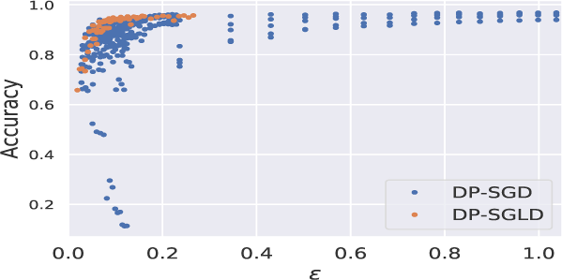
Performance of DP-SGLD within DP-SGD family, on MNIST with CNN. Here δ = 10⁻⁵,|B| = 256, η_SGD = 0.25, η_SGLD = 10⁻⁵, epoch ≤ 15, C ∈ [0.5, 5], σ_SGD ∈ [0.5, 3].

Furthermore, DP-SGLD is generalizable to any network architecture (whenever DP-SGD works) and to any weight prior distribution (via different regularization terms); DP-SGLD does not require the computation of the complicated KL divergence. Computationally speaking, DP-SGLD enjoys fast computation speed (i.e. low computation complexity) since the per-sample gradient clipping can be very efficiently calculated using the outer product method [14,29], the fastest acceleration technique of DP deep learning implemented in Opacus library. For example, on MNIST in Section 5, DP-SGLD requires only 10 sec/epoch, while DP-BBP takes 480 sec/epoch since it is incompatible with outer product.

However, DP-SGLD only offers empirical weight distribution{w_t}, which is not analytic and requires large memory for storage in order to give sufficiently accurate uncertainty quantification (e.g. we record 100 iterations of w_t in Figure 7 and 1000 iterations in Figure 4). The memory burden can be too large to scale to large models that have billions of parameters, such as GPT-2.

Fig. 4:

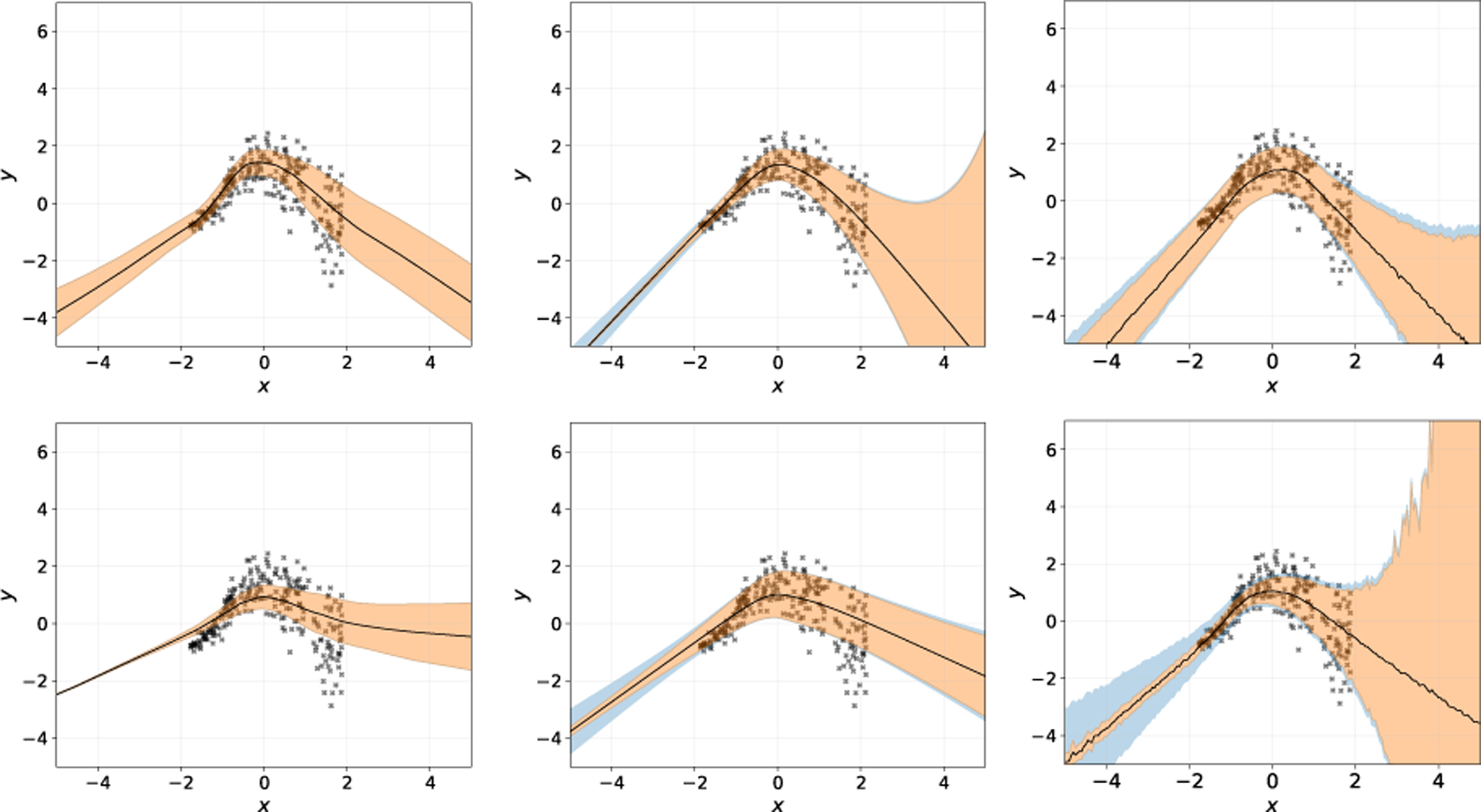
Prediction uncertainty on heteroscedasticity regression with Gaussian priors. Left to right: SGLD, BBP, MC Dropout. Upper: non-DP BNNs. Lower: DP-BNNs. Orange region refers to the posterior uncertainty. Blue region refers to the data uncertainty. Black line is the mean prediction.

4.2. Differentially Private Bayes by BackPropagation

Our DP-BBP can be viewed as DP-SGD working on the distributional hyperparameters such as the mean and the variance. In fact, it is the only method that does not works on weights directly, and thus requires to work with KL divergence via the variational inference problem (2).

$$\begin{array}{l}\overline{\underset{¯}{\mathbf{Algorithm\; 3:}\text{ Differentially private Bayes\hspace{0.17em}by\hspace{0.17em}BackPropagation (DP-BBP)\hspace{0.17em}\hspace{0.17em}\hspace{0.17em}\hspace{0.17em}\hspace{0.17em}\hspace{0.17em}\hspace{0.17em}\hspace{0.17em}\hspace{0.17em}\hspace{0.17em}\hspace{0.17em}\hspace{0.17em}\hspace{0.17em}\hspace{0.17em}\hspace{0.17em}\hspace{0.17em}\hspace{0.17em}\hspace{0.17em}\hspace{0.17em}\hspace{0.17em}\hspace{0.17em}\hspace{0.17em}\hspace{0.17em}\hspace{0.17em}\hspace{0.17em}\hspace{0.17em}}}}\\ \mathbf{Input:}\text{ Examples }\left\{\left({\mathit{\text{x}}}_i,y_i\right)\right\},\text{\hspace{0.17em}loss\hspace{0.17em}}{ℒ}_{\text{BBP}}\left(\cdot ;\theta \right).\\ \mathbf{for}t=1toT\mathbf{do}\\ \text{\hspace{1em}\hspace{1em}Randomly\hspace{0.17em}sample\hspace{0.17em}a\hspace{0.17em}batch\hspace{0.17em}}{B}_t\subset \left\{1,2,\dots ,n\right\};\\ \mathbf{for}i\in B\mathbf{do}\\ \mathbf{for}j=1toN\mathbf{do}\\ \text{\hspace{1em}\hspace{1em}\hspace{1em}\hspace{1em}Sample\hspace{0.17em}}{w}^{\left(j\right)}\text{\hspace{0.17em}from\hspace{0.17em}}q\left(w|{\theta }_{t-1}\right)\text{\hspace{0.17em}and\hspace{0.17em}compute}\\ g_i^{\left(j\right)}={\nabla }_{\theta }{ℒ}_{\text{BBP}}\left(x_i,y_i;w^{\left(j\right)},\theta \right);\\ \text{\hspace{1em}\hspace{1em}\hspace{1em}Define\hspace{0.17em}}{\overline{g}}_i=\frac{1}{N}{\sum }_j{g}_i^{\left(j\right)}\text{\hspace{0.17em}and\hspace{0.17em}clip\hspace{0.17em}}{\tilde{g}}_i=\min \left\{1,\frac{C_t}{{‖{\overline{g}}_i‖}_2}\right\}\cdot {\overline{g}}_i;\\ \text{\hspace{1em}\hspace{1em}Add\hspace{0.17em}noise\hspace{0.17em}}\widehat{g}=\frac{1}{\left|B_t\right|}{\sum }_{i\in B}{\tilde{g}}_i+\frac{\sigma \cdot C_t}{\left|B_t\right|}\cdot 𝒩\left(0,I_d\right).\\ \text{\hspace{1em}\hspace{1em}Update\hspace{0.17em}}{\theta }_t\leftarrow {\theta }_{t-1}-{\eta }_t\widehat{g};\\ \underset{¯}{\mathbf{Output:}{\theta }_T}\end{array}$$

There are three major drawbacks of DP-BBP due to the KL divergence approach. Firstly, the updating rule needs significant modification for each type of network layers, e.g. convolutional layers and embedding layers. Therefore DP-BBP cannot work flexibly on general NNs. Secondly, DP-BBP suffers from high computation complexity. Under Gaussian variational distributions, DP-BBP needs to compute two hyperparameters (mean and standard deviation) for a single parameter (weight), which doubles the complexity of DP-SGLD, DP-MC Dropout and DP-SGD. The computational issue is further exacerbated due to the N samplings of w^(j) from q(w|θ_t), which means the number of backpropagation is N times that of DP-SGLD and DP-MC Dropout. This introduces an inevitable tradeoff: when N is larger, DP-BBP tends to be more accurate but its computational complexity is also higher, leading to the overall inefficiency of DP-BBP. Thirdly, DP-BBP cannot be accelerated by the outer product method as it violates the supported network layers². Since the per-sample gradient clipping is the computational bottleneck for acceleration, DP-BBP can be too slow to be practically useful if the computation consideration overweighs its utility.

As for its advantages, DP-BBP is compatible to general DP optimizers such as DP-Adam. Similar to DP-SGLD, the DP-BBP can flexibly work under various priors by using different regularization terms r(w) inside ${ℒ}_{\text{BBP}}$. Moreover, in sharp contrast to DP-SGLD and DP-MC Dropout, which only describe the weight distribution empirically, the distributional hyperparameters updated by DP-BBP directly characterize an analytic weight distribution for inference.

4.3. Differentially Private Monte Carlo Dropout

We can view our DP-MC Dropout as applying DP-SGD (or any other DP optimizers) on any NN with dropout layers, and thus DP-MC Dropout enjoys the low computation costs provided by the outer product acceleration in Opacus. Regarding the uncertainty quantification, DP-MC Dropout offers the empirical weight distribution at low storage costs since only w_T is stored, which means that its posterior is not analytic and will not be accurate if the number of training iterations is not sufficiently large.

$$\begin{array}{l}\overline{\underset{¯}{\mathbf{Algorithm\; 4:}\text{ Differentially private MC\hspace{0.17em}Dropout (DP-MC\hspace{0.17em}Dropout)\hspace{0.17em}\hspace{0.17em}\hspace{0.17em}\hspace{0.17em}\hspace{0.17em}\hspace{0.17em}\hspace{0.17em}\hspace{0.17em}\hspace{0.17em}\hspace{0.17em}\hspace{0.17em}\hspace{0.17em}\hspace{0.17em}\hspace{0.17em}\hspace{0.17em}\hspace{0.17em}\hspace{0.17em}\hspace{0.17em}\hspace{0.17em}\hspace{0.17em}\hspace{0.17em}\hspace{0.17em}\hspace{0.17em}\hspace{0.17em}\hspace{0.17em}\hspace{0.17em}\hspace{0.17em}\hspace{0.17em}\hspace{0.17em}\hspace{0.17em}\hspace{0.17em}\hspace{0.17em}\hspace{0.17em}\hspace{0.17em}\hspace{0.17em}\hspace{0.17em}\hspace{0.17em}\hspace{0.17em}\hspace{0.17em}\hspace{0.17em}\hspace{0.17em}\hspace{0.17em}}}}\\ \mathbf{Input:}\text{ Examples }\left\{\left({\mathit{\text{x}}}_i,y_i\right)\right\},\text{\hspace{0.17em}loss\hspace{0.17em}}{ℒ}_{\text{Dropout}}\left(\cdot ;\mathit{w}\right),\text{\hspace{0.17em}regularization\hspace{0.17em}}r\left(\mathit{w}\right).\\ \mathbf{for}t=1toT\mathbf{do}\\ \text{\hspace{1em}\hspace{1em}Randomly\hspace{0.17em}sample\hspace{0.17em}a\hspace{0.17em}batch\hspace{0.17em}}{B}_t\subset \left\{1,2,\dots ,n\right\};\\ \text{\hspace{1em}\hspace{1em}Randomly drop out some weights and denote the remained as\hspace{0.17em}}{\mathit{w}}_{t-1};\\ \mathbf{for}i\in B_t\mathbf{do}\\ \text{\hspace{1em}\hspace{1em}\hspace{1em}Compute\hspace{0.17em}}{g}_i={\nabla }_{\mathit{w}}{ℒ}_{\text{Dropout}}\left({\text{x}}_i,y_i;{\mathit{w}}_{t-1}\right)\\ \text{\hspace{1em}\hspace{1em}\hspace{1em}Clip\hspace{0.17em}}{\tilde{g}}_i=\min \left\{1,\frac{C_t}{{‖g_i‖}_2}\right\}\cdot g_i.;\\ \text{\hspace{1em}\hspace{1em}Add\hspace{0.17em}noise\hspace{0.17em}}\widehat{g}=\frac{1}{\left|B_t\right|}{\sum }_{i\in B_t}{\tilde{g}}_i+\frac{\sigma \cdot C_t}{\left|B_t\right|}\cdot 𝒩\left(0,I_d\right)\\ \text{\hspace{1em}\hspace{1em}Update\hspace{0.17em}}{\mathit{w}}_t\leftarrow {\mathit{w}}_{t-1}-{\eta }_t\left(\widehat{g}+{\nabla }_{\mathit{w}}r\left({\mathit{w}}_{t-1}\right)\right);\\ \underset{¯}{\mathbf{Output:}{\mathit{w}}_T}\end{array}$$

A limitation to the theory of MC Dropout [13] is that the equivalence between the empirical risk minimization of ${ℒ}_{\text{Dropout}}$ and the KL divergence minimization (2) no longer holds beyond the Gaussian weight prior. Nevertheless, algorithmically speaking, DP-MC Dropout also works with other priors by using different regularization terms.

4.4. Analysis of Privacy

The following theorem gives the privacy loss ϵ by the GDP accountant [10,5].

Theorem 2 (Theorem 5 in [5]). For both DP-MC Dropout and DP-BBP, under any DP-optimizers (e.g. DP-SGD, DP-Adam, DP-HeavyBall) with the number of iterations T, noise scale σ and batch size |B|, the resulting neural network is $\sqrt{T\left(e^{1/{\sigma }^2}-1\right)}\left|B\right|/n-GDP$.

We remark that, from [10, Corollary 2.13], μ-GDP can be mapped to $\left(ϵ,\delta \right)\text{-DP}$ via $\delta \left(\epsilon ;\mu \right)=\Phi \left(-\epsilon /\mu +\mu /2\right)-{\text{e}}^{\epsilon }\Phi \left(-\epsilon /\mu -\mu /2\right)$. As alternatives to GDP, other privacy accountants such as the Moments Accountant (MA) [1,26,9,2] can be applied to characterize ϵ, though implicitly (see Appendix A). Since DP-MC Dropout and DP-BBP do not quantify the uncertainty via optimizers, all privacy accountants give the same ϵ as training DP-SGD on regular NNs. We next give the privacy of DP-SGLD by writing it as DP-SGD.

Theorem 3. For DP-SGLD with the number of iterations T, learning rate η, batch size |B| and clipping norm C, the resulting neural network is $\sqrt{T\left(e^{n^2\eta C^2/{\left|B\right|}^2}-1\right)}\left|B\right|/n-GDP$.

The proof follows from Theorem 1 and [5, Theorem 5], given in Appendix D. We observe sharp contrast between Theorem 2 and Theorem 3: (1) while the clipping norm C and learning rate η have no effect on the privacy guarantee of DP-MC Dropout and DP-BBP, these hyperparameters play important roles in DP-SGLD. For instance, the learning rate triggers a tradeoff: larger η converges faster but smaller η is more private; see Figure 2. (2) To get stronger privacy guarantee, DP-MC Dropout and DP-BBP need smaller T and larger σ; however, DP-SGLD needs smaller T, C and η. (3) Surprisingly, the batch size |B| has opposite effects in DP-SGLD and in other methods: DP-SGLD with larger |B| is more private, while smaller |B| amplifies the privacy for DP-SGD [3,33,17,10].

Fig. 2:

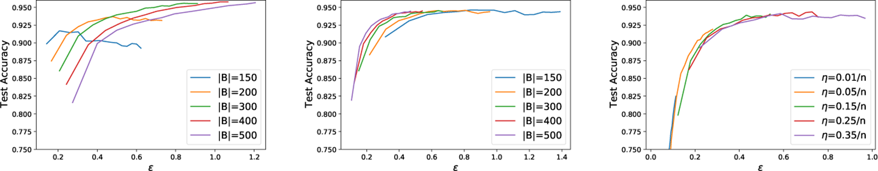
Effects of batch size and learning rate on DP-SGD (left) and DP-SGLD (middle & right) with CNNs on MNIST. See Appendix C.3 for settings.

5. Experiments

We further evaluate the proposed DP-BNNs on the classification (MNIST) and regression tasks, based on performance measures including uncertainty quantification, computational speed and privacy-accuracy tradeoff. In particular, we observe that DP-SGLD tends to outperform DP-MC Dropout, DP-BBP and DP-SGD, with little reduction in performance compared to non-DP models. All experiments (except BBP) are run with Opacus library under Apache License 2.0 and on Google Colab with a P100 GPU. A detailed description of the experiments can be found in Appendix C. Code of our implementation is available at https://github.com/littlekii/DPBBP.

5.1. Classification on MNIST

We first evaluate three DP-BNNs on the MNIST dataset, which contains n = 60000 training samples and 10000 test samples of 28 × 28 grayscale images of hand-written digits.

Accuracy and Privacy

While all of non-DP methods have similar high test accuracy, in the DP regime in Table 1, DP-SGLD outperforms other Bayesian and non-Bayesian methods under almost identical privacy budgets (for details, see Appendix C). For the multilayer perceptron (MLP), all BNNs (DP or non-DP) do not lose much accuracy when gaining the ability to quantify uncertainty, compared to the non-Bayesian SGD. However, DP comes at high cost of accuracy, except for DP-SGLD which does not deteriorate comparing to its non-DP version, while other methods experience an accuracy drop ≈ 20%. Furthermore, DP-SGLD enjoys clear advantage in accuracy on more complicated convolutional neural network (CNN).

Table 1:

Test accuracy and running time of DP-BBP, DP-SGLD, DP-MC Dropout, DP-SGD, and their non-DP counterparts. We use a default two-layer MLP and additionally a four-layer CNN by Opacus in parentheses.

Methods	Weight Prior	DP Time/Epoch	DP accuracy	Non-DP accuracy
SGLD	Gaussian  Laplacian	10s 10s	0.90 (0.95) 0.89 (0.89)	0.95 (0.96) 0.90 (0.89)
BBP	Gaussian Laplacian	480s 480s	0.80 (——) 0.81 (——)	0.97 (——) 0.98 (——)
MC Dropout	Gaussian	9s	0.78 (0.77)	0.98 (0.97)
SGD (non-Bayesian)	——	10s	0.77 (0.95)	0.97 (0.99)

Uncertainty and Calibration

Regarding uncertainty quantification, we visualize the empirical prediction posterior of Bayesian MLPs in Figure 7 over 100 predictions on a single image. Note that at each probability (x-axis), we plot a cluster of bins each of which represents a class³. For example, the left-most cluster represents not predicting a class. As a measure of the reliability, the calibration [28,16] measures the distance between a classification model’s accuracy and its prediction probability, i.e. confidence. Formally, denoting the vector of prediction probability for the i-th sample as π_i, the confidence for this sample is ${\text{conf}}_i={\max }_k{\left[{\pi }_i\right]}_k$ and the prediction is ${\text{pred}}_i=\arg {\max }_k{\left[{\pi }_i\right]}_k$. Two commonly applied calibration errors are the expected calibration error (ECE) and the maximum calibration error (MCE) [16].

Concretely, in the left-bottom plot, DP-SGLD has low red (class 3) and brown (class 5) bins on the left-most cluster, meaning it will predict 3 or 5. We see that non-DP BNNs usually predict correctly (with a low red bin in the left-most cluster), though the posterior probabilities of the correct class are different across three BNNs. Obviously, DP changes the empirical posterior probabilities significantly in distinct ways. First, all DP-BNNs are prone to make mistakes in prediction, e.g. both DP-SGLD and DP-BBP tend to predict class 5. In fact, DP-SGLD are equally likely to predict class 3 and 5 yet DP-BBP seldom predicts class 3 anymore, when DP is enforced. Additionally, DP-SGLD is less confident about its mistake compared to DP-BBP. This is indicated by the small x-coordinate of the right-most bins, and implies that DP-SGLD can be more calibrated, as discussed in the next paragraph. For MC Dropout, DP also reduces the confidence in predicting class 3 but the mistaken prediction spreads over several classes. Hence the quality of uncertainty quantification provided by DP-MC Dropout lies between that by DP-SGLD and DP-BBP.

Ideally, a reliable classifier should be calibrated in the sense that the accuracy matches the confidence. When a model is highly confident in its prediction yet it is not accurate, such classifier is over-confident; otherwise it is under-confident. It is well-known that the regular NNs are over-confident [16,25] and (non-DP) BNNs are more calibrated [24]. In Table 2 and Table 4, we again test the two-layer MLP and four-layer CNN on MNIST, with or without Gaussian prior under DP-BNNs regime. Notice that in the BNN regime, training with weight decay is equivalent to adopting a Gaussian prior, while training without weight decay is equivalent to using a non-informative prior.

Table 2:

Calibration errors of SGLD, BBP, MC Dropout, SGD, and their DP counterparts on MNIST with two-layer MLP, with or without Gaussian prior.

Methods	DP-ECE	DP-MCE	Non-DP ECE	Non-DP MCE
BBP (w/ prior)	0.204	0.641	0.024	0.052
BBP (w/o prior)	0.167	0.141	0.166	0.166
SGLD (w/ prior)	0.007	0.175	0.035	0.175
SGLD (w/o prior)	0.126	0.465	0.008	0.289
MC Dropout (w/ prior)	0.008	0.080	0.030	0.041
MC Dropout (w/o prior)	0.078	0.225	0.002	0.725
SGD (w/ prior)	0.013	0.089	0.016	0.139
SGD (w/o prior)	0.106	0.625	0.005	0.299

On MLP, the Gaussian prior (or weight decay) significantly improves the MCE, in the non-DP regime and furthermore in the DP regime (see Figure 8). However, on CNN, while the Gaussian prior helps in the non-DP regime, this may not hold true in the DP regime. For both neural network structures, DP exacerbates the mis-calibration: leading to worse MCE when the non-informative prior is used. See lower panel of Figure 8 and Figure 9. However, this is usually not the case when DP is guaranteed under the Gaussian prior. Additionally, BNNs often enjoy smaller MCE than the regular MLP but may have larger MCE than the regular CNN. In the case of SGLD, the effect of DP-BNN and prior distribution is visualized in Figure 3.

Fig. 3:

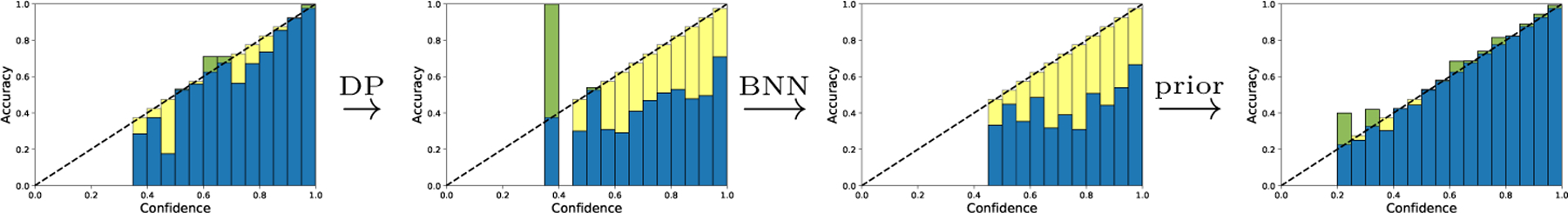
Reliability diagram on MNIST with two-layer MLP, using SGD, DP-SGD and DP-SGLD (right two).

5.2. Heteroscedastic synthetic data regression

We compare the prediction uncertainty of BNNs on the heteroscedastic data generated from Gaussian process (see details in Appendix C). Here, the prediction uncertainty for each data point is estimated by the empirical posterior over 1000 predictions. Specifically, the prediction uncertainty can be decomposed into the posterior uncertainty (also called epistemic uncertainty, the blue region) and the data uncertainty (also called aleatoric uncertainty, the orange region), whose mathematical formulation is delayed in Appendix C. In Figure 4, all three non-DP BNNs (upper panel) characterize similar prediction uncertainty, regarded as the ground truth.

In our experiments, we train all BNNs with DP-GD for 200 epochs and noise multiplier such that the DP is $ϵ=4.21$, $\delta =1/250$. As shown in Table 3, SGLD is surprisingly accurate in both DP and non-DP scenarios while BBP and MC Dropout suffer notably from DP, even though their non-DP versions are accurate.

Table 3:

Mean square error of heteroscedasticity regression with Gaussian prior. The reported error is the median over 20 independent simulations.

Methods	DP	Non-DP
SGLD	0.510	0.523
BBP	1.276	0.562
MC Dropout	0.682	0.591

Clearly, the prediction uncertainty of SGLD and BBP are barely affected by DP; additionally, given that DP-SGLD has much better mean squared error, this experiment confirms that DP-SGLD is more desirable for uncertainty quantification with DP guarantee. Unfortunately, for MC Dropout, DP leads to substantially greater posterior uncertainty and unstable mean prediction. The resulting wide out-of-sample predictive intervals provide little information.

6. Discussion

This work proposes three DP-BNNs, namely DP-SGLD, DP-BBP and DP-MC Dropout, to both quantify the model uncertainty and guarantee the privacy in deep learning. Our work also provides valuable insights about the connection between DP-SGLD, a method often applied in the Bayesian settings, and DP-SGD, which is widely used without the consideration of Bayesian inference. This connection reveals novel findings about the impact of training hyperparameters on DP-SGLD, e.g. larger batch size enhances the privacy. All three DP-BNNs are evaluated through multiple metrics and demonstrate their advantages and limitations, supported by both theoretical and empirical analyses. For instance, as a sampling method, DP-SGLD outperforms the optimization methods, DP-BBP and DP-MC Dropout, on classification and regression tasks, at little expense of performance in comparison to the non-Bayesian or non-DP counterparts. However, DP-SGLD requires a possibly long period of burn-in to converge and its uncertainty quantification requires storing hundreds of weights, making the method less scalable.

For future directions, it is of interest to extend the connection between DP-SGD and DP-SGLD to a more general class, i.e. DP-SG-MCMC. Particularly, the convergence and generalization behaviors of DP-BNNs needs more investigation, similar to the analysis of different DP linear regression [32].

References

- 1.Abadi M, Chu A, Goodfellow I, McMahan HB, Mironov I, Talwar K, Zhang L: Deep learning with differential privacy. In: Proceedings of the 2016 ACM SIGSAC conference on computer and communications security pp. 308–318 (2016) [Google Scholar]
- 2.Asoodeh S, Liao J, Calmon FP, Kosut O, Sankar L: A better bound gives a hundred rounds: Enhanced privacy guarantees via f-divergences. In: 2020 IEEE International Symposium on Information Theory (ISIT) pp. 920–925. IEEE; (2020) [Google Scholar]
- 3.Balle B, Barthe G, Gaboardi M: Privacy amplification by subsampling: Tight analyses via couplings and divergences. arXiv preprint arXiv:1807.01647 (2018)
- 4.Blundell C, Cornebise J, Kavukcuoglu K, Wierstra D: Weight uncertainty in neural network. In: International Conference on Machine Learning pp. 1613–1622. PMLR; (2015) [Google Scholar]
- 5.Bu Z, Dong J, Long Q, Su WJ: Deep learning with gaussian differential privacy. Harvard data science review 2020(23) (2020) [DOI] [PMC free article] [PubMed] [Google Scholar]
- 6.Bu Z, Gopi S, Kulkarni J, Lee YT, Shen JH, Tantipongpipat U: Fast and memory efficient differentially private-sgd via jl projections. arXiv preprint arXiv:2102.03013 (2021)
- 7.Buntine WL: Bayesian backpropagation. Complex systems 5, 603–643 (1991) [Google Scholar]
- 8.Cadwalladr C, Graham-Harrison E: Revealed: 50 million facebook profiles harvested for cambridge analytica in major data breach. The guardian 17, 22 (2018) [Google Scholar]
- 9.Canonne C, Kamath G, Steinke T: The discrete gaussian for differential privacy. arXiv preprint arXiv:2004.00010 (2020)
- 10.Dong J, Roth A, Su WJ: Gaussian differential privacy. arXiv preprint arXiv:1905.02383 (2019)
- 11.Dwork C, McSherry F, Nissim K, Smith A: Calibrating noise to sensitivity in private data analysis. In: Theory of cryptography conference pp. 265–284. Springer; (2006) [Google Scholar]
- 12.Dwork C, Roth A, et al. : The algorithmic foundations of differential privacy. Foundations and Trends in Theoretical Computer Science 9(3–4), 211–407 (2014) [Google Scholar]
- 13.Gal Y, Ghahramani Z: Dropout as a bayesian approximation: Representing model uncertainty in deep learning. In: international conference on machine learning pp. 1050–1059. PMLR; (2016) [Google Scholar]
- 14.Goodfellow I: Efficient per-example gradient computations. arXiv preprint arXiv:1510.01799 (2015)
- 15.Graves A: Practical variational inference for neural networks. Advances in neural information processing systems 24 (2011) [Google Scholar]
- 16.Guo C, Pleiss G, Sun Y, Weinberger KQ: On calibration of modern neural networks. In: International Conference on Machine Learning pp. 1321–1330. PMLR; (2017) [Google Scholar]
- 17.Kasiviswanathan SP, Lee HK, Nissim K, Raskhodnikova S, Smith A: What can we learn privately? SIAM Journal on Computing 40(3), 793–826 (2011) [Google Scholar]
- 18.Koskela A, Jälkö J, Honkela A: Computing tight differential privacy guarantees using fft. In: International Conference on Artificial Intelligence and Statistics pp. 2560–2569. PMLR; (2020) [Google Scholar]
- 19.Kuleshov V, Fenner N, Ermon S: Accurate uncertainties for deep learning using calibrated regression. In: International Conference on Machine Learning pp. 2796–2804. PMLR; (2018) [Google Scholar]
- 20.Li B, Chen C, Liu H, Carin L: On connecting stochastic gradient mcmc and differential privacy. In: The 22nd International Conference on Artificial Intelligence and Statistics pp. 557–566. PMLR; (2019) [Google Scholar]
- 21.Li C, Chen C, Carlson D, Carin L: Preconditioned stochastic gradient langevin dynamics for deep neural networks. In: Proceedings of the AAAI Conference on Artificial Intelligence vol. 30 (2016) [Google Scholar]
- 22.MacKay DJ: A practical bayesian framework for backpropagation networks. Neural computation 4(3), 448–472 (1992) [Google Scholar]
- 23.MacKay DJ: Probable networks and plausible predictions—a review of practical bayesian methods for supervised neural networks. Network: computation in neural systems 6(3), 469–505 (1995) [Google Scholar]
- 24.Maroñas J, Paredes R, Ramos D: Calibration of deep probabilistic models with decoupled bayesian neural networks. Neurocomputing 407, 194–205 (2020) [Google Scholar]
- 25.Minderer M, Djolonga J, Romijnders R, Hubis F, Zhai X, Houlsby N, Tran D, Lucic M: Revisiting the calibration of modern neural networks. arXiv preprint arXiv:2106.07998 (2021)
- 26.Mironov I, Talwar K, Zhang L: R\ ‘enyi differential privacy of the sampled gaussian mechanism. arXiv preprint arXiv:1908.10530 (2019)
- 27.Neal RM: Bayesian learning for neural networks, vol. 118. Springer Science & Business Media; (2012) [Google Scholar]
- 28.Niculescu-Mizil A, Caruana R: Predicting good probabilities with supervised learning. In: Proceedings of the 22nd international conference on Machine learning pp. 625–632 (2005) [Google Scholar]
- 29.Rochette G, Manoel A, Tramel EW: Efficient per-example gradient computations in convolutional neural networks. arXiv preprint arXiv:1912.06015 (2019)
- 30.Ryffel T, Trask A, Dahl M, Wagner B, Mancuso J, Rueckert D, PasseratPalmbach J: A generic framework for privacy preserving deep learning. arXiv preprint arXiv:1811.04017 (2018)
- 31.Srivastava N, Hinton G, Krizhevsky A, Sutskever I, Salakhutdinov R: Dropout: a simple way to prevent neural networks from overfitting. The journal of machine learning research 15(1), 1929–1958 (2014) [Google Scholar]
- 32.Wang YX: Revisiting differentially private linear regression: optimal and adaptive prediction & estimation in unbounded domain. arXiv preprint arXiv:1803.02596 (2018)
- 33.Wang YX, Balle B, Kasiviswanathan SP: Subsampled rényi differential privacy and analytical moments accountant. In: The 22nd International Conference on Artificial Intelligence and Statistics pp. 1226–1235. PMLR; (2019) [Google Scholar]
- 34.Wang YX, Fienberg S, Smola A: Privacy for free: Posterior sampling and stochastic gradient monte carlo. In: International Conference on Machine Learning pp. 2493–2502. PMLR; (2015) [Google Scholar]
- 35.Welling M, Teh YW: Bayesian learning via stochastic gradient langevin dynamics. In: Proceedings of the 28th international conference on machine learning (ICML-11) pp. 681–688. Citeseer; (2011) [Google Scholar]
- 36.Xiong HY, Barash Y, Frey BJ: Bayesian prediction of tissue-regulated splicing using rna sequence and cellular context. Bioinformatics 27(18), 2554–2562 (2011) [DOI] [PubMed] [Google Scholar]
- 37.Zeiler MD, Fergus R: Stochastic pooling for regularization of deep convolutional neural networks. arXiv preprint arXiv:1301.3557 (2013)
- 38.Zhang Z, Rubinstein B, Dimitrakakis C: On the differential privacy of bayesian inference. In: Proceedings of the AAAI Conference on Artificial Intelligence vol. 30 (2016) [Google Scholar]
Associated Data
This section collects any data citations, data availability statements, or supplementary materials included in this article.