

Summary
We develop a Bayesian nonparametric (BNP) approach to evaluate the causal effect of treatment in a randomized trial where a nonterminal event may be censored by a terminal event, but not vice versa (i.e., semi-competing risks). Based on the idea of principal stratification, we define a novel estimand for the causal effect of treatment on the nonterminal event. We introduce identification assumptions, indexed by a sensitivity parameter, and show how to draw inference using our BNP approach. We conduct simulation studies and illustrate our methodology using data from a brain cancer trial. The R code implementing our model and algorithm is available for download at https://github.com/YanxunXu/BaySemiCompeting.
Keywords: Bayesian nonparametrics, Brain cancer trial, Causal inference, Identification assumptions, Principal stratification, Sensitivity analysis
1. Introduction
Semi-competing risks (Fine and others, 2001) occur in studies where observation of a nonterminal event (e.g., progression) may be pre-empted by a terminal event (e.g., death), but not vice versa. In randomized clinical trials to evaluate treatments of life-threatening diseases, patients are often observed for specific types of disease progression and survival. Often, the primary outcome is patient survival, resulting in data analyses focusing on the terminal event using standard survival analysis tools (Ibrahim and others, 2005). However, there may also be interest in understanding the causal effect of treatment on nonterminal outcomes such as progression, readmission, etc. An example is a randomized trial for the treatment of malignant brain tumors, where one of the important progression endpoints is based on deterioration of the cerebellum. An important feature of this progression endpoint is that it is biologically plausible that a patient could die without cerebellar deterioration. Thus, analyzing the effect of treatment on progression needs to account for the fact that progression is not well-defined after death.
Varadhan and others (2014) review
models that have been proposed for analyzing semi-competing data. These models can be
classified into two broad categories: models for the distribution of the observable data,
e.g., cause-specific hazards, subdistribution functions (Fix
and Neyman, 1951; Hougaard, 1999; Xu and others, 2010; Lee and others, 2015), and models for
the distribution of the latent failure times (Robins,
1995a,b; Lin
and others, 1996; Wang,
2003; Peng and Fine, 2007; Ding and others, 2009; Peng and Fine, 2012; Chen,
2012; Hsieh and Huang, 2012; Comment and others, 2019). Xu and others (2010) argued against the
use of latent failure time models because the marginal distribution of the nonterminal event
is hypothetical. This is because the joint distribution of the nonterminal event
( ) and terminal event
(
) and terminal event
( ) is only identified on a wedge of
 . Rather, they argued that “semi-competing
risks data are better modeled using an illness-death compartment model,” where “a subject
can either transit directly to the terminal event or first to the nonterminal event and then
to the terminal event.” They proposed a Markov shared frailty model for the transition
rates. Lee and others (2015)
proposed a Bayesian semi-parametric extension, which focused on estimation of regression
parameters, characterization of dependence between event times and prediction of event times
for specific covariate profiles. The latent failure approaches of Fine and others (2001), Wang (2003), and Peng and Fine (2007) have
focused on estimating regression parameters and estimating dependence between nonterminal
and terminal event times using copula models. Robins
(1995a,b) focused solely on estimating
regression parameters and discusses causal interpretability. Recently, Comment and others (2019) proposed a casual estimand
similar to the one we discuss here, but uses different models (i.e., parametric frailty
models) and different causal assumptions (i.e., latent ignorability).
. Rather, they argued that “semi-competing
risks data are better modeled using an illness-death compartment model,” where “a subject
can either transit directly to the terminal event or first to the nonterminal event and then
to the terminal event.” They proposed a Markov shared frailty model for the transition
rates. Lee and others (2015)
proposed a Bayesian semi-parametric extension, which focused on estimation of regression
parameters, characterization of dependence between event times and prediction of event times
for specific covariate profiles. The latent failure approaches of Fine and others (2001), Wang (2003), and Peng and Fine (2007) have
focused on estimating regression parameters and estimating dependence between nonterminal
and terminal event times using copula models. Robins
(1995a,b) focused solely on estimating
regression parameters and discusses causal interpretability. Recently, Comment and others (2019) proposed a casual estimand
similar to the one we discuss here, but uses different models (i.e., parametric frailty
models) and different causal assumptions (i.e., latent ignorability).
In this article, we are interested in estimating the causal effect of treatment on the nonterminal endpoint from a randomized trial generating semi-competing risk data. Using the potential outcomes framework (Rubin, 1974), we propose a principal stratification estimand (Frangakis and Rubin, 2002) to quantify the causal effect. Our estimand is a time-varying version of the survival average causal effect (see, e.g., Zhang and Rubin, 2003; Tchetgen Tchetgen, 2014), quantified on a relative risk scale. We introduce assumptions that utilize baseline covariates to identify this estimand from the distribution of the observable data and propose a Bayesian nonparametric (BNP) approach for modeling this distribution. An important feature of BNP models is their large support. For example, a Dirichlet process (Ferguson and others, 1973) location-scale mixture of normals (one of the most widely used BNP models), has full support on the space of absolutely continuous distributions (Lo, 1984). To handle covariates, our approach is based on the dependent Dirichlet process (DDP) prior introduced by MacEachern (1999).
The article is outlined as follows: Section 2 introduces the motivating brain tumor study. The formal definition of the causal estimand is introduced in Section 3. We introduce the BNP model in Section 4. A simulation study is summarized in Section 5. We analyze the brain tumor data in Section 6, and conclude with brief discussion in Section 7.
2. Motivating brain tumor study
The methodology is motivated by a randomized and placebo-controlled Phase II trial for 222 recurrent gliomas patients, who were scheduled for tumor resection with recurrent malignant brain tumors (Brem and others, 1995). Eligible patients had a single focus of tumor in the cerebrum, had a Karnofsky score greater than 60, had completed radiation therapy, had not taken nitrosoureas within 6 weeks of enrollment, and had not had systematic chemotherapy within 4 weeks of enrollment. The data include 11 baseline prognostic measures and a baseline evaluation of cerebellar function. The former includes age, race, Karnofsky performance score, local vs. whole brain radiation, percent of tumor resection, previous use of nitrosoureas, and tumor histology (glioblastoma, anapestic astrocytoma, oligodendrolioma, or other) at implantation. Patients were randomized to receive surgically implanted biodegradable polymer discs with or without 3.85% of carmustine. The follow-up duration was 1 year. Of the 219 patients with complete baseline measures, 204 were observed to die and 100 were observed to progress prior to death. Of the 15 patients who did not die, 4 were observed to have cerebellar progression. Our goal is to estimate the causal effect of treatment on time to cerebellar progression.
3. Causal estimand and identification assumptions
3.1. Potential outcomes and causal estimand
Let  ,
,  , and
, and
 denote progression time, death time,
and censoring time, under treatment
denote progression time, death time,
and censoring time, under treatment  . Here,
 represents control and treatment
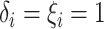
group, respectively. All event times are log-transformed. Fundamental to our setting is
that
represents control and treatment
group, respectively. All event times are log-transformed. Fundamental to our setting is
that  (i.e., progression
cannot happen after death).
(i.e., progression
cannot happen after death).
The causal estimand of interest is the function
| (3.1) |
where  is a smooth function of
 . Among patients who survive to time
 under both treatments, this estimand
contrasts the risk of progression prior to time
under both treatments, this estimand
contrasts the risk of progression prior to time  for treatment 1 relative
to treatment 0, which is a causal effect in a subgroup defined by potential outcomes. This
estimand is an example of a principal stratum causal effect (Frangakis and Rubin, 2002).
for treatment 1 relative
to treatment 0, which is a causal effect in a subgroup defined by potential outcomes. This
estimand is an example of a principal stratum causal effect (Frangakis and Rubin, 2002).
3.2. Observed data
Let  denote treatment assignment and
 denote a vector of the
baseline covariates. Let
denote a vector of the
baseline covariates. Let  ,
,  , and
, and  .
Let
.
Let  ,
,
 ,
,
 , and
, and
 denote the observed event
times and event indicators. The observed data for each patient are
denote the observed event
times and event indicators. The observed data for each patient are
 .
We assume that we observe
.
We assume that we observe  i.i.d. copies of
 . Throughout, variables
subscripted by
. Throughout, variables
subscripted by  will denote data specific to patient
 .
.
3.3. Identification assumptions
We introduce the following four assumptions that are sufficient for identifying our causal estimand.
Assumption 1: Treatment is randomized, i.e.,
 |
and  .
.
This obviously holds by design in randomized trials as considered here.
Assumption 2: Censoring is noninformative in the sense that
 |
and  for all
  .
.
Let  and
and
 denote the conditional
hazard function and conditional distribution function of
denote the conditional
hazard function and conditional distribution function of  given
given  ,
respectively. Under Assumptions 1 and 2,
,
respectively. Under Assumptions 1 and 2,  and
and  are identified via the
following formulae:
are identified via the
following formulae:
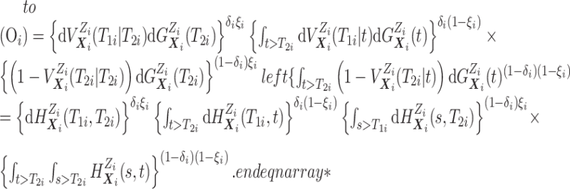
 |
and
| (3.2) |
Furthermore, the conditional subdistribution function of  given
given  and
and  ,
,
 , is identified via the
following formula:
, is identified via the
following formula:
| (3.3) |
where  . Together
 and
and
 identify the
joint subdistribution
identify the
joint subdistribution  for
for
 given
given
 .
.
Assumption 3: The conditional joint distribution function of
 given
given
 ,
,
 , follows a Gaussian
copula model, i.e.,
, follows a Gaussian
copula model, i.e.,
| (3.4) |
where  is a standard normal c.d.f. and
 is a bivariate normal c.d.f.
with mean 0, marginal variances 1, and correlation
is a bivariate normal c.d.f.
with mean 0, marginal variances 1, and correlation  . For
fixed
. For
fixed  ,
,  is identified since
 and
and
 are identified.
Similar assumptions have been used in the causal mediation literature (Daniels and others, 2012).
are identified.
Similar assumptions have been used in the causal mediation literature (Daniels and others, 2012).
Assumption 4: Progression time under treatment  is
conditionally independent of death time under treatment
is
conditionally independent of death time under treatment  given
death time under treatment
given
death time under treatment  and covariates
  , i.e.,
 |
Under Assumptions 1–4,  is identified from the
distribution of the observed data as follows:
is identified from the
distribution of the observed data as follows:
| (3.5) |
where  is the empirical
distribution of
is the empirical
distribution of  .
.
4. Bayesian regression model
In this section, we propose a BNP survival regression model on the unknown conditional (on
 ) distribution
of
) distribution
of  . However, any alternative
Bayesian survival regression models could be implemented (Hanson and Johnson, 2002; Gelfand and Kottas,
2003; Zhou and Hanson, 2018; Sparapani and others, 2016; Xu and others, 2019); however, the first
three are restrictive in how covariates are entered and the fourth one is
semi-parametric.
. However, any alternative
Bayesian survival regression models could be implemented (Hanson and Johnson, 2002; Gelfand and Kottas,
2003; Zhou and Hanson, 2018; Sparapani and others, 2016; Xu and others, 2019); however, the first
three are restrictive in how covariates are entered and the fourth one is
semi-parametric.
4.1. Dependent Dirichlet process—Gaussian process prior
We start with a review of the Dirichlet process (DP) as a prior for an unknown distribution and step by step extend it to the dependent Dirichlet process—Gaussian process prior.
The DP prior has been widely used as a prior model for a random unknown probability
distribution. We write  if a random
distribution
if a random
distribution  of a
of a  -dimensional random vector
 follows a DP prior, where
 is known as the total mass parameter
and
is known as the total mass parameter
and  is known as the base measure. Sethuraman (1994) provides a constructive definition of
a DP, where
is known as the base measure. Sethuraman (1994) provides a constructive definition of
a DP, where  ,
,
 ,
,
 and
and  .
In many applications, the discrete nature of
.
In many applications, the discrete nature of  is not appropriate. A DP
mixture model extends the DP model by replacing each point mass
is not appropriate. A DP
mixture model extends the DP model by replacing each point mass  with
a continuous kernel. For example, a DP mixture of normals takes the form:
with
a continuous kernel. For example, a DP mixture of normals takes the form:
 ,
where
,
where  is the density function of a multivariate normal random vector with mean vector
 and variance–covariance
matrix
and variance–covariance
matrix  .
.
To introduce a prior on the conditional (on covariates  ) distribution
(
) distribution
( ) of
) of
 , the DP mixture model has
been extended to a dependent DP (DDP) by replacing
, the DP mixture model has
been extended to a dependent DP (DDP) by replacing  in each term with
 ,
which is a multivariate stochastic process indexed by
,
which is a multivariate stochastic process indexed by  . A DDP mixture of normals
takes the form:
. A DDP mixture of normals
takes the form:
| (4.6) |
To complete the prior specification, we need to posit a stochastic process prior for
 .
A common specification are independent Gaussian process (GP) priors (MacEachern, 1999; Xu and
others, 2016) on
.
A common specification are independent Gaussian process (GP) priors (MacEachern, 1999; Xu and
others, 2016) on  .
A GP prior is specified such that for all
.
A GP prior is specified such that for all  and
(
and
( ,
the distribution of
,
the distribution of  follows a multivariate normal distribution with mean vector
  and
and  covariance matrix where the
 entry is
  ).
We write
).
We write  .
For an extensive review of the GP priors, see Rasmussen
and Williams (2006) and MacKay (1999). We
model the mean function
.
For an extensive review of the GP priors, see Rasmussen
and Williams (2006) and MacKay (1999). We
model the mean function  as a linear regression on
covariates
as a linear regression on
covariates  with covariance process specified as
| (4.7) |
where  is the dimension of the covariate vector,
 and
and
 is a small constant (e.g.,
 ) used to ensure that the
covariance function is positive definite. To ensure a reasonable covariance structure,
continuous covariates should be standardized to have mean 0 and variance 1. More flexible
covariance functions can be considered if desired. Additional priors are introduced on the
) used to ensure that the
covariance function is positive definite. To ensure a reasonable covariance structure,
continuous covariates should be standardized to have mean 0 and variance 1. More flexible
covariance functions can be considered if desired. Additional priors are introduced on the
 ’s and
 , the details of which
are discussed in Appendix A.1. We write
, the details of which
are discussed in Appendix A.1. We write
 .
.
4.2. Application to semi-competing risks data
Separately for each treatment group  , we posit independent
DDP-GP’s on the unknown conditional (on
, we posit independent
DDP-GP’s on the unknown conditional (on  ) probability
measure (
) probability
measure ( ) of
) of
 . Since
 (
( ) and
) and  ,
the prior on
,
the prior on  induces priors on
 and
and
 (identified under
Assumptions 1 and 2) and together with the Gaussian copula for
(identified under
Assumptions 1 and 2) and together with the Gaussian copula for  implies a prior on the
estimand
implies a prior on the
estimand  . The prior on
 also induces priors on
non-identified quantities which have no impact on our analysis. More specifics about our
prior are presented in Appendix A.1.
also induces priors on
non-identified quantities which have no impact on our analysis. More specifics about our
prior are presented in Appendix A.1.
Before transitioning to the posterior sampling algorithm, note that the relevant portion
of the observed data likelihood for individual  , with data
 is
is
 |
We include the second equality because it allows us to see that, using data augmentation
to replace the integrals, the joint full data likelihood is  .
This will allow us to use existing posterior simulation techniques for DDP-GP models.
.
This will allow us to use existing posterior simulation techniques for DDP-GP models.
4.3. Posterior simulation
The details of the Markov chain Monte Carlo (MCMC) algorithm are presented in Appendix
A.2. Here, we focus on individuals assigned to
treatment  and suppress the dependence of the
notation on
and suppress the dependence of the
notation on  . As noted above, the MCMC implementation
is based on the full data likelihood. While
. As noted above, the MCMC implementation
is based on the full data likelihood. While  is an infinite
mixture of normals, we approximate it by a finite mixture with
is an infinite
mixture of normals, we approximate it by a finite mixture with  components. This finite mixture
model for
components. This finite mixture
model for  can be replaced by a
hierarchical model where (1)
can be replaced by a
hierarchical model where (1)  is a latent variable that selects
mixture component
is a latent variable that selects
mixture component  (
( ) with probability
 (properly normalized to handle the
finite number of mixture components) and (2) given
(properly normalized to handle the
finite number of mixture components) and (2) given  , the pair
  follows a multivariate normal
distribution with mean
follows a multivariate normal
distribution with mean  and variance
  .
.
Posterior simulation is based on this hierarchical model characterization. Importantly, all of the full conditionals in the MCMC algorithm have a closed form representation. Details of the MCMC posterior simulation can be found in Appendix A.2.
5. Simulation studies
5.1. Simulation setup
We considered three simulation scenarios to evaluate the performance of our proposed
approach with 500 repeated simulations for each scenario. We generated
 . Independently of
 , we generated two independent covariates
 and
and  ,
where
,
where  followed a truncated normal
distribution with mean 4.5, variance 1, and truncation interval
followed a truncated normal
distribution with mean 4.5, variance 1, and truncation interval  and
and  . For the first two
simulation scenarios, we simulated progression time and death time on the log scale as
follows:
. For the first two
simulation scenarios, we simulated progression time and death time on the log scale as
follows:
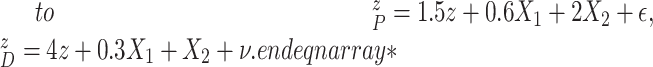 |
In Scenario 1, we assumed  followed a bivariate normal
distribution with mean
followed a bivariate normal
distribution with mean  , marginal variances
 , and correlation
 In Scenario 2, we assumed
 to be a scaled multivariate
 distribution with degree of freedom
 , mean
  , marginal variance
 , and correlation
 . Scenario 3 explored
performance under a nonlinear covariate effect specification on progression and death
times. We generated
. Scenario 3 explored
performance under a nonlinear covariate effect specification on progression and death
times. We generated  and
and
 ,
with
,
with  following the same
distribution as in Scenario 1.
following the same
distribution as in Scenario 1.
In all scenarios, the censoring time  on the log scale was
generated independently according to a
on the log scale was
generated independently according to a  distribution. In Scenario 1, 56.6% of the patients’ deaths and progressions were both
observed (
distribution. In Scenario 1, 56.6% of the patients’ deaths and progressions were both
observed ( ), 2% of the patients’ deaths
and progressions were both censored (
), 2% of the patients’ deaths
and progressions were both censored ( ), 36.4% of
the patients’ deaths were observed and progressions were censored
(
), 36.4% of
the patients’ deaths were observed and progressions were censored
( ), 5% of the patients’
deaths were censored and progressions were observed (
), 5% of the patients’
deaths were censored and progressions were observed ( ). In Scenario 2, 55.8% of the
patients’ deaths and progressions were both observed, 4.8% of the patients’ deaths and
progressions were both censored, 33.6% of the patients’ deaths were observed and
progressions were censored, 5.8% of the patients’ deaths were censored and progressions
were observed. In Scenario 3, these percentages were 69.4%, 3.4%, 10.6%, and 16.6%,
respectively. For the joint distribution of
). In Scenario 2, 55.8% of the
patients’ deaths and progressions were both observed, 4.8% of the patients’ deaths and
progressions were both censored, 33.6% of the patients’ deaths were observed and
progressions were censored, 5.8% of the patients’ deaths were censored and progressions
were observed. In Scenario 3, these percentages were 69.4%, 3.4%, 10.6%, and 16.6%,
respectively. For the joint distribution of  and
and
 in (3.4), we set
  in the
Gaussian copula as the truth. We generated
in the
Gaussian copula as the truth. We generated  for
for
 independent patients and then
coarsened to
independent patients and then
coarsened to  .
.
To explore sensitivity of  with respect to
 , we conducted inference for
 under several values of
 . For all three
scenarios, we specified hyperparameters as described in Appendix A.1.
. For all three
scenarios, we specified hyperparameters as described in Appendix A.1.
For comparative purposes, we implemented two alternative models. The first one is a naive
Bayesian (Naive) model by assuming that the conditional probability measure
( of
of
 follows a multivariate
normal distribution with mean
follows a multivariate
normal distribution with mean  and variance–covariance matrix
  , with
conjugate multivariate normal priors on
, with
conjugate multivariate normal priors on  and
and  and an inverse
Wishart prior on
and an inverse
Wishart prior on  (i.e.,
 ,
,
 ,
and
,
and  ,
,
 ). The second one is the linear
dependent DDP (LinearDDP) model proposed in De Iorio
and others (2009), which simplifies the proposed BNP model by
assuming that
). The second one is the linear
dependent DDP (LinearDDP) model proposed in De Iorio
and others (2009), which simplifies the proposed BNP model by
assuming that  in
(4.6) is a linear regression on
in
(4.6) is a linear regression on
 , instead of a Gaussian
process prior on
, instead of a Gaussian
process prior on  used
in the proposed BNP model.
used
in the proposed BNP model.
For each analysis, we ran 5000 MCMC iterations with an initial burn-in of 2000 iterations and a thinning factor of 10. The convergence diagnostics using the R package coda show no evidence of practical convergence problems.
5.2. Simulation results
We first report on the performance in terms of recovering the true treatment-specific
marginal survival functions for time to death. For the BNP approach, Figure 1 shows, for each of the three simulation scenarios and by
treatment group (first and second rows refer to treatments 0 and 1, respectively), the
true survival functions (solid line), the posterior mean survival functions averaged over
simulated data sets (dashed line), and 95% point-wise credible intervals (computed using
quantiles) averaged over simulated data sets (dotted lines) on the original time scale
(days). As another metric of performance, we computed, for each simulated data set, the
root mean squared error (RMSE) taken as the square root of the average of the squared
errors at 34 equally spaced grid points in log-scaled time interval
 . For each scenario, Table 1(a) summarizes the mean and standard deviation
of RMSE across the 500 simulated data sets. Both Figure
1 and Table 1(a) show that our proposed
BNP procedure performs well, for each of the three scenarios, in terms of recovering the
true survival function.
. For each scenario, Table 1(a) summarizes the mean and standard deviation
of RMSE across the 500 simulated data sets. Both Figure
1 and Table 1(a) show that our proposed
BNP procedure performs well, for each of the three scenarios, in terms of recovering the
true survival function.
Fig. 1.

For each simulation scenario and by treatment group (first and second rows refer to treatments 0 and 1, respectively), the true survival functions (solid line), the posterior mean survival functions averaged over simulated data sets (dashed line), and 95% point-wise credible intervals (computed using quantiles) averaged over simulated data sets (dotted lines). Survival times are on the original scale (days).
Table 1.
(a) For each scenario, mean and standard deviation of RMSE across 500 simulated data
sets under the proposed BNP method, the naive Bayesian method (Naive), and the
LinearDDP method. Bold values indicate that the proposed BNP yields the smallest mean
RMSE when  . (b) Means and standard
deviations of RMSE for estimating
. (b) Means and standard
deviations of RMSE for estimating  across
500 simulations in three scenarios under the proposed BNP approach, the naive Bayesian
method (Naive), and the LinearDDP method, respectively
across
500 simulations in three scenarios under the proposed BNP approach, the naive Bayesian
method (Naive), and the LinearDDP method, respectively
| Scenario |

|

|
|||||
|---|---|---|---|---|---|---|---|
| BNP | Naive | LinearDDP | BNP | Naive | LinearDDP | ||
| 1 | 0.012 (0.007) | 0.013 (0.007) | 0.014 (0.007) | 0.012 (0.006) | 0.013 (0.007) | 0.015 (0.008) | (a) |
| 2 | 0.042 (0.022) | 0.088 (0.032) | 0.063 (0.020) | 0.019 (0.007) | 0.073 (0.035) | 0.058 (0.023) | |
| 3 | 0.012 (0.006) | 0.013 (0.007) | 0.014 (0.007) | 0.012 (0.007) | 0.014 (0.007) | 0.016 (0.008) | |
| Scenario |

|

|
|||||
|---|---|---|---|---|---|---|---|
| BNP | Naive | LinearDDP | BNP | Naive | LinearDDP | ||
| 1 | 0.286 (0.087) | 0.328 (0.126) | 0.332 (0.087) | 0.059 (0.035) | 0.073 (0.051) | 0.091 (0.016) | |
| 2 | 0.277 (0.128) | 0.493 (0.250) | 0.449 (0.189) | 0.090 (0.062) | 0.199 (0.169) | 0.179 (0.123) | |
| 3 | 0.106 (0.032) | 0.105 (0.038) | 0.115 (0.043) | 0.033 (0.016) | 0.035 (0.021) | 0.043 (0.027) | |
| Scenario |

|
|||
|---|---|---|---|---|
| BNP | Naive | LinearDDP | ||
| 1 | 0.185 (0.037) | 0.207 (0.047) | 0.181 (0.042) | (b) |
| 2 | 0.261 (0.070) | 0.243 (0.111) | 0.203 (0.084) | |
| 3 | 0.086 (0.028) | 0.097 (0.034) | 0.086 (0.035) | |
Table 1(a) also shows the mean and standard deviation of RMSE for the Naive and the LinearDDP models. In Scenario 1, the two models match the true simulation model, thereby yielding comparable results as the proposed BNP model. In contrast, the Naive and the LinearDDP models perform worse than the BNP model in Scenario 2 when the fitted model does not match the simulation truth. In Scenario 3, the BNP model performs slightly better than the Naive and the LinearDDP models. Overall, the proposed BNP model is more robust compared to the Naive and the LinearDDP models.
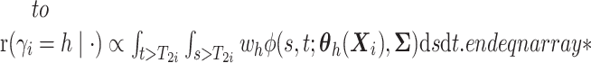
Evaluation of  requires evaluation of
 as the second marginal
under
as the second marginal
under  . Expression (3.5) allows us now to estimate
 . Both the numerator and denominator
can be evaluated as functionals of the currently imputed random probability measure
. Both the numerator and denominator
can be evaluated as functionals of the currently imputed random probability measure
 of time
to log progression
of time
to log progression  and time to log death
 under treatment
 , marginalizing with respect to the
empirical distribution of covariates
, marginalizing with respect to the
empirical distribution of covariates  ’s. Each
iteration of the posterior MCMC simulation evaluates a point-wise estimate and we estimate
the posterior mean of
’s. Each
iteration of the posterior MCMC simulation evaluates a point-wise estimate and we estimate
the posterior mean of  as
as  across iterations. We also report the mean RMSE in estimating the
 by averaging over 500
repeated simulations under the proposed BNP, the Naive, and the LinearDDP models. Table 1(b) summarizes the results.
by averaging over 500
repeated simulations under the proposed BNP, the Naive, and the LinearDDP models. Table 1(b) summarizes the results.
Figure 2 shows  versus
 in the three scenarios, respectively,
using
in the three scenarios, respectively,
using  and
and  . As
shown in Figure 2, in all three scenarios, when
. As
shown in Figure 2, in all three scenarios, when
 , the estimates under the
proposed BNP model reliably recover the simulated true
, the estimates under the
proposed BNP model reliably recover the simulated true  and avoid the excessive bias seen with other
  values. This agrees
with the results reported in Table 1(b) that
values. This agrees
with the results reported in Table 1(b) that
 always yields the smallest mean
RMSE in all three scenarios. Furthermore, when
always yields the smallest mean
RMSE in all three scenarios. Furthermore, when  , the proposed
BNP model has smaller mean RMSE compared to the Naive and the LinearDDP models. When
, the proposed
BNP model has smaller mean RMSE compared to the Naive and the LinearDDP models. When
 or
or  , the
BNP model performs better or comparable to the Naive model in terms of providing smaller
mean RMSE and variability of RMSE across simulations.
, the
BNP model performs better or comparable to the Naive model in terms of providing smaller
mean RMSE and variability of RMSE across simulations.
Fig. 2.

The posterior estimates (dashed lines) of  versus
 on the original scale (days) for the
three scenarios using
on the original scale (days) for the
three scenarios using  , respectively. The
solid lines represent the simulation truth using
, respectively. The
solid lines represent the simulation truth using  . The dotted lines represent
95% point-wise credible intervals (computed using quantiles) averaged over simulated
datasets.
. The dotted lines represent
95% point-wise credible intervals (computed using quantiles) averaged over simulated
datasets.
6. Brain tumor data analysis
An initial analysis of the brain tumor death outcome using Kaplan–Meier is given in Figure 3, indicating that the treatment group has higher
estimated survival probabilities. The estimated difference at 365 days is 2.6% (95% CI
 8.1% to 13.3%). Figure 3 plots the estimated posterior survival curves for treatment and control
groups marginalized over the distribution of covariate with 95% credible intervals; panels
(a), (b), and (c) display the results for the BNP, Naive, and LinearDDP approaches,
respectively. Using the BNP approach, the estimated posterior difference in survival at 365
days is 6.2% (95% CI
8.1% to 13.3%). Figure 3 plots the estimated posterior survival curves for treatment and control
groups marginalized over the distribution of covariate with 95% credible intervals; panels
(a), (b), and (c) display the results for the BNP, Naive, and LinearDDP approaches,
respectively. Using the BNP approach, the estimated posterior difference in survival at 365
days is 6.2% (95% CI  1.2% to 13.3%). For the Naive approach, the
estimated posterior difference in survival at 365 days is 8.4% (95% CI 0.2% to 17.9%). The
LinearDDP approach estimated the posterior difference in survival at 365 days to be 9.9%
(95% CI 0.9% to 20.8%). The BNP approach produces comparable or higher treatment-specific
estimates of survival and greater treatment differences than Kaplan–Meier. In contrast, the
Naive and LinearDDP approaches produce comparable or lower (higher) estimate of survival for
the control (treatment) group than Kaplan–Meier. Comparatively speaking, the Naive and
LinearDDP approaches produce lower treatment-specific posterior estimates of survival than
the BNP approach. When we compare the fit to the observed survival data of the three
approaches using the log-pseudo marginal likelihood (LPML; (Geisser and Eddy, 1979), a leave-one-out cross-validation statistic, we see the
BNP performs better. Specifically, the LPML for the treatment arm is
1.2% to 13.3%). For the Naive approach, the
estimated posterior difference in survival at 365 days is 8.4% (95% CI 0.2% to 17.9%). The
LinearDDP approach estimated the posterior difference in survival at 365 days to be 9.9%
(95% CI 0.9% to 20.8%). The BNP approach produces comparable or higher treatment-specific
estimates of survival and greater treatment differences than Kaplan–Meier. In contrast, the
Naive and LinearDDP approaches produce comparable or lower (higher) estimate of survival for
the control (treatment) group than Kaplan–Meier. Comparatively speaking, the Naive and
LinearDDP approaches produce lower treatment-specific posterior estimates of survival than
the BNP approach. When we compare the fit to the observed survival data of the three
approaches using the log-pseudo marginal likelihood (LPML; (Geisser and Eddy, 1979), a leave-one-out cross-validation statistic, we see the
BNP performs better. Specifically, the LPML for the treatment arm is
 144,
144,  161,
161,
 147 for the BNP, Naive, and LinearDDP
approaches, respectively. The corresponding numbers for the control arm are
147 for the BNP, Naive, and LinearDDP
approaches, respectively. The corresponding numbers for the control arm are
 137,
137,  174, and
 139.
139.
Fig. 3.

The dashed lines in (a) represent the estimated posterior mean survival curves for the proposed BNP method. The dotdash lines in (b) and (c) represent the estimated posterior mean survival curves for the Naive method and LinearDDP method, respectively. In all figures, the solid lines represent the Kaplan–Meier curves of the observed survival data in control and treatment groups, and the dotted lines represent 95% point-wise credible intervals of the posterior estimated survival curves. Survival times are on the original scale (days).
For the BNP (panel (a)), Naive (panel (b)), and LinearDDP (panel (c)) approaches, Figure 4 plots the posterior estimates (along with
point-wise 95% credible intervals) of the causal estimand  versus
  for three choices of
 , 0.2, 0.5, and 0.8. Except near
 , there are no appreciable differences
between the two approaches. In addition, the results are insensitive to choice of
, there are no appreciable differences
between the two approaches. In addition, the results are insensitive to choice of
 . Overall, this analysis shows that there
is a lower estimated risk of progression for treatment versus of control at all time points,
except near zero. However, there is appreciable uncertainty, characterized by wide posterior
credible intervals, that precludes more definitive conclusions about the difference between
treatment groups with regards to progression. When we compare the fit to the observed
survival and progression data of the BNP and Naive approaches using LPML,
we see that the approaches perform comparably. Specifically, the LPML for the treatment arm
is
. Overall, this analysis shows that there
is a lower estimated risk of progression for treatment versus of control at all time points,
except near zero. However, there is appreciable uncertainty, characterized by wide posterior
credible intervals, that precludes more definitive conclusions about the difference between
treatment groups with regards to progression. When we compare the fit to the observed
survival and progression data of the BNP and Naive approaches using LPML,
we see that the approaches perform comparably. Specifically, the LPML for the treatment arm
is  227,
227,  232, and
 235 for the BNP, Naive, and LinearDDP
approaches, respectively. The corresponding numbers for the control arm are
235 for the BNP, Naive, and LinearDDP
approaches, respectively. The corresponding numbers for the control arm are
 215,
215,  214, and
 219.
219.
Fig. 4.

Posterior estimated  versus
  on
the original scale (days) in brain tumor data analysis for different
on
the original scale (days) in brain tumor data analysis for different
 ’s under the proposed BNP method, the
Naive method, and the LinearDDP method, respectively. The solid lines represent the
posterior estimated
’s under the proposed BNP method, the
Naive method, and the LinearDDP method, respectively. The solid lines represent the
posterior estimated  , and the dashed lines represent
95% point-wise credible intervals. (a) BNP, (b) Naive, and (c) LinearDDP.
, and the dashed lines represent
95% point-wise credible intervals. (a) BNP, (b) Naive, and (c) LinearDDP.
7. Discussion
In this article, we proposed a causal estimand for characterizing the effect of treatment
on progression in a randomized trials with a semi-competing risks data structure. We
introduced a set of identification assumptions, indexed by a non-identifiable sensitivity
parameter that quantifies the correlation between survival under treatment and survival
under control. Selecting a range of the sensitivity parameter  in a
specific trial will depend on clinical considerations. For example, in trial of a biomarker
targeted therapy, one might expect weaker correlation, since survival under control might be
primarily determined by co-morbidities and the survival under treatment might be more
determined by the presence of the targeted molecular aberration. For example, a recent
FDA-approved drug LOXO-101 (Hyman and
others, 2017) targeting NTRK fusion has an overall response rate of 78%
in the treatment group, while only 10% in the control group. In contrast, for some
chemotherapies, the same factors that impact survival under control may equally impact
survival under treatment, e.g., co-morbidities, social support (Kaufman and others, 2015). Then we would suggest a
medium or high
in a
specific trial will depend on clinical considerations. For example, in trial of a biomarker
targeted therapy, one might expect weaker correlation, since survival under control might be
primarily determined by co-morbidities and the survival under treatment might be more
determined by the presence of the targeted molecular aberration. For example, a recent
FDA-approved drug LOXO-101 (Hyman and
others, 2017) targeting NTRK fusion has an overall response rate of 78%
in the treatment group, while only 10% in the control group. In contrast, for some
chemotherapies, the same factors that impact survival under control may equally impact
survival under treatment, e.g., co-morbidities, social support (Kaufman and others, 2015). Then we would suggest a
medium or high  , say
, say  .
Fortunately, the sensitivity parameter is bounded between
.
Fortunately, the sensitivity parameter is bounded between  1 and 1
and, in most settings, should be positive; a range should be selected in close collaboration
with subject matter experts.
1 and 1
and, in most settings, should be positive; a range should be selected in close collaboration
with subject matter experts.
We proposed a flexible BNP approach for modeling the distribution of the observed data.
Since the causal estimand is a functional of the distribution of the observed data and
 , we draw inference about it using
posterior summarization. Our procedure can easily be extended to accommodate a prior
distribution on
, we draw inference about it using
posterior summarization. Our procedure can easily be extended to accommodate a prior
distribution on  , which will allow for integrated
inference. Our procedure also allows for posterior inferences about other identified causal
contrasts such as the distribution of survival under treatment versus under control. The
procedure can also be used for predictive inference for patients with specific covariate
profiles.
, which will allow for integrated
inference. Our procedure also allows for posterior inferences about other identified causal
contrasts such as the distribution of survival under treatment versus under control. The
procedure can also be used for predictive inference for patients with specific covariate
profiles.
Acknowledgments
The authors would like to thank Drs Henry Brem and Steven Piantadosi for providing access to data from the brain cancer trial. Conflict of Interest: None declared.
Appendix A
A.1 Determining prior hyperparameters
As priors for  in the GP
mean function, we assume
in the GP
mean function, we assume 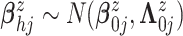 .
We assume
.
We assume 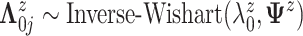 ,
where
,
where 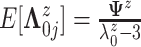 .
The precision parameter
.
The precision parameter  in the DDP is assumed to be
distributed
in the DDP is assumed to be
distributed  .
.
In applications of Bayesian inference with small to moderate sample sizes, a critical
step is to fix values for all hyperparameters  .
Inappropriate information could be introduced by improper numerical values, leading to
inaccurate posterior inference. We use an empirical Bayes method to obtain
.
Inappropriate information could be introduced by improper numerical values, leading to
inaccurate posterior inference. We use an empirical Bayes method to obtain
 by fitting a bivariate normal distribution for responses of patients under treatment
 ,
,  .
For
.
For  , we assume a
diagonal matrix with the diagonal values being 10. After an empirical estimate of
, we assume a
diagonal matrix with the diagonal values being 10. After an empirical estimate of
 is computed, we tune
 and
and
 so that the prior mean of
 matches the
empirical estimate,
matches the
empirical estimate,  and
and
 .
Finally, we assume
.
Finally, we assume  .
.
A.2 MCMC computational details
Unless required for clarity, we suppress dependence of the notation on treatment
 . Here,
  is
used to denote endpoint (
is
used to denote endpoint ( for progression and
 for death). We define
 |
Let  and
and
 ,
,
 ,
,
 (
( ),
),
 is an
is an
 matrix where the
 th row contains the
 -dimensional covariate vector
 for the
 th patient,
  is an
is an
 matrix where the
 entry is
 ,
,
 is an
is an
 matrix where the
 th row refers to the
 th patient in
 , the
, the  th
column refers to patient
th
column refers to patient  and
and  element is the indicator that the
patient in
element is the indicator that the
patient in  th row is the same as the patient in
the
th row is the same as the patient in
the  th column,
  is an
is an
 identity matrix,
 where
where 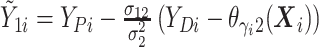 and
and 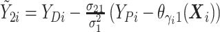 ,
,
 ,
and
,
and  .
.
For  , we iterate through the following
six updating steps:
, we iterate through the following
six updating steps:
- (1) Update

here
 is
the number of observations such that
is
the number of observations such that  . Then,
 and
and
 .
. -
(2) Update
 Assuming that
 ,
,
here
 is generated from Step 1.
 - (3) Update


- (4) Update
 ,
,

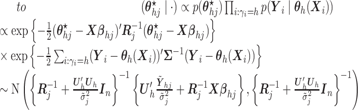
- (5) Update

here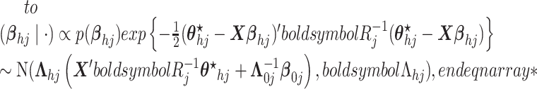
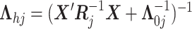 .
. -
(6) Update
 , where
 .
.We write
 as
as  where
where  includes
 .
.- If

 is point mass at
  .
. - If
 (i.e.,
 ),
),
here
 .
. - If
 and
and


here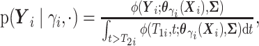
 .
. - If
 and
and


here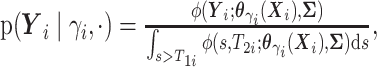
 .
.
Contributor Information
Yanxun Xu, Department of Applied Mathematics and Statistics, Johns Hopkins University, 3400 N. Charles Street, Baltimore, MD 21218, USA yanxun.xu@jhu.edu.
Daniel Scharfstein, Department of Biostatistics, Johns Hopkins University, 615 N Wolfe St, Baltimore, MD 21205, USA.
Peter Müller, Department of Mathematics, The University of Texas at Austin, 2515 Speedway, RLM 8.100, Austin, TX 78712, USA.
Michael Daniels, Department of Statistics, University of Florida, Union Rd, Gainesville, FL 32603, USA.
Funding
This research is supported by National Institute Health NIH CA183854 and NIH GM 112327, and National Science Foundation NSF1918854.
References
- Brem, H., Piantadosi, S., Burger, P. C., Walker, M., Selker, R., Vick, N. A., Black, K., Sisti, M., Brem, S., Mohr, G.. and others. (1995). Placebo-controlled trial of safety and efficacy of intraoperative controlled delivery by biodegradable polymers of chemotherapy for recurrent gliomas. The Lancet 345, 1008–1012. [DOI] [PubMed] [Google Scholar]
- Chen, Y.-H. (2012). Maximum likelihood analysis of semicompeting risks data with semiparametric regression models. Lifetime Data Analysis 18, 36–57. [DOI] [PubMed] [Google Scholar]
- Comment, L., Mealli, F., Haneuse, S. and Zigler, C. (2019). Survivor average causal effects for continuous time: a principal stratification approach to causal inference with semicompeting risks. arXiv preprint arXiv:1902.09304. [Google Scholar]
- Daniels, M. J., Roy, J. A., Kim, C., Hogan, J. W. and Perri, M. G. (2012). Bayesian inference for the causal effect of mediation. Biometrics 68, 1028–1036. [DOI] [PMC free article] [PubMed] [Google Scholar]
- De Iorio, M., Johnson, W. O., Müller, P. and Rosner, G. L. (2009). Bayesian nonparametric nonproportional hazards survival modeling. Biometrics 65, 762–771. [DOI] [PMC free article] [PubMed] [Google Scholar]
- Ding, A., Shi, G., Wang, W. and Hsieh, J.-J. (2009). Marginal regression analysis for semi-competing risks data under dependent censoring. Scandinavian Journal of Statistics 36, 481–500. [Google Scholar]
- Ferguson, T. S. (1973). A Bayesian analysis of some nonparametric problems. The Annals of Statistics 1, 209–230. [Google Scholar]
- Fine, J. P., Jiang, H. and Chappell, R. (2001). On semi-competing risks data. Biometrika 88, 907–919. [Google Scholar]
- Fix, E. and Neyman, J. (1951). A simple stochastic model of recovery, relapse, death and loss of patients. Human Biology, 205–241. [PubMed] [Google Scholar]
- Frangakis, C. E. and Rubin, D. B. (2002). Principal stratification in causal inference. Biometrics 58, 21–29. [DOI] [PMC free article] [PubMed] [Google Scholar]
- Geisser, S. and Eddy, W. F. (1979). A predictive approach to model selection. Journal of the American Statistical Association 74, 153–160. [Google Scholar]
- Gelfand, A. E. and Kottas, A. (2003). Bayesian semiparametric regression for median residual life. Scandinavian Journal of Statistics 30, 651–665. [Google Scholar]
- Hanson, T. and Johnson, W. O. (2002). Modeling regression error with a mixture of Polya trees. Journal of the American Statistical Association 97, 1020–1033. [Google Scholar]
- Hougaard, P. (1999). Multi-state models: a review. Lifetime Data Analysis 5, 239–264. [DOI] [PubMed] [Google Scholar]
- Hsieh, J.-J. and Huang, Y.-T. (2012). Regression analysis based on conditional likelihood approach under semi-competing risks data. Lifetime Data Analysis 18, 302–320. [DOI] [PubMed] [Google Scholar]
- Hyman, D. M., Laetsch, T. W., Kummar, S., DuBois, S. G., Farago, A. F., Pappo, A. S., Demetri, G. D., El-Deiry, W. S., Lassen, U. N., Dowlati, A.. and others. (2017). The efficacy of larotrectinib (LOXO-101), a selective tropomyosin receptor kinase (TRK) inhibitor, in adult and pediatric TRK fusion cancers. Journal of Clinical Oncology 18_suppl, LBA2501. [Google Scholar]
- Ibrahim, J. G., Chen, M.-H. and Sinha, D. (2005). Bayesian Survival Analysis. Hoboken, NJ: Wiley Online Library. [Google Scholar]
- Kaufman, P. A, Awada, A., Twelves, C., Yelle, L., Perez, E. A., Velikova, G., Olivo, M. S., He, Y., Dutcus, C. E. and Cortes, J. (2015). Phase III open-label randomized study of eribulin mesylate versus capecitabine in patients with locally advanced or metastatic breast cancer previously treated with an anthracycline and a taxane. Journal of Clinical Oncology 33, 594. [DOI] [PMC free article] [PubMed] [Google Scholar]
- Lee, K. H., Haneuse, S., Schrag, D. and Dominici, F. (2015). Bayesian semiparametric analysis of semicompeting risks data: investigating hospital readmission after a pancreatic cancer diagnosis. Journal of the Royal Statistical Society: Series C (Applied Statistics) 64, 253–273. [DOI] [PMC free article] [PubMed] [Google Scholar]
- Lin, D. Y., Robins, J. M. and Wei, L. J. (1996). Comparing two failure time distributions in the presence of dependent censoring. Biometrika 83, 381–393. [Google Scholar]
- Lo, A. Y. (1984). On a class of Bayesian nonparametric estimates: I. Density estimates. The Annals of Statistics 12, 351–357. [Google Scholar]
- MacEachern, S. N. (1999). Dependent nonparametric processes. In: ASA Proceedings of the Section on Bayesian Statistical Science. Alexandria, VA: American Statistical Association, pp. 50–55. [Google Scholar]
- MacKay, D. (1999). Introduction to Gaussian processes. Technical Report. Cambridge University. http://wol.ra.phy.cam.ac.uk/mackay/GP/.ter. [Google Scholar]
- Peng, L. and Fine, J. P. (2007). Regression modeling of semicompeting risks data. Biometrics 63, 96–108. [DOI] [PubMed] [Google Scholar]
- Peng, L. and Fine, J. P. (2012). Rank estimation of accelerated lifetime models with dependent censoring. Journal of the American Statistical Association. [Google Scholar]
- Rasmussen, C. E. and Williams, C. K. I. (2006). Gaussian Processes for Machine Learning. MIT Press. [Google Scholar]
- Robins, J. M. (1995a). An analytic method for randomized trials with informative censoring: Part II. Lifetime Data Analysis 1, 417–434. [DOI] [PubMed] [Google Scholar]
- Robins, J. M. (1995b). An analytic method for randomized trials with informative censoring: Part 1. Lifetime Data Analysis 1, 241–254. [DOI] [PubMed] [Google Scholar]
- Rubin, D. B. (1974). Estimating causal effects of treatments in randomized and nonrandomized studies. Journal of Educational Psychology 66, 688. [Google Scholar]
- Sethuraman, J. (1994). A constructive definition of Dirichlet priors. Statistica Sinica 4, 639–650. [Google Scholar]
- Sparapani, R. A., Logan, B. R., McCulloch, R. E. and Laud, P. W. (2016). Nonparametric survival analysis using Bayesian Additive Regression Trees (BART). Statistics in Medicine 35, 2741–2753. [DOI] [PMC free article] [PubMed] [Google Scholar]
- Tchetgen Tchetgen, E. J. (2014). Identification and estimation of survivor average causal effects. Statistics in Medicine 33, 3601–3628. [DOI] [PMC free article] [PubMed] [Google Scholar]
- Varadhan, R., Xue, Q.-L. and Bandeen-Roche, K. (2014). Semicompeting risks in aging research: methods, issues and needs. Lifetime Data Analysis 20, 538–562. [DOI] [PMC free article] [PubMed] [Google Scholar]
- Wang, W. (2003). Estimating the association parameter for copula models under dependent censoring. Journal of the Royal Statistical Society: Series B (Statistical Methodology) 65, 257–273. [Google Scholar]
- Xu, J., Kalbfleisch, J. D. and Tai, B. (2010). Statistical analysis of illness–death processes and semicompeting risks data. Biometrics 66, 716–725. [DOI] [PubMed] [Google Scholar]
- Xu, Y., Müller, P., Wahed, A. S. and Thall, P. F. (2016). Bayesian nonparametric estimation for dynamic treatment regimes with sequential transition times. Journal of the American Statistical Association 111, 921–950. [DOI] [PMC free article] [PubMed] [Google Scholar]
- Xu, Y., Thall, P. F., Hua, W. and Andersson, B. S. (2019). Bayesian non-parametric survival regression for optimizing precision dosing of intravenous busulfan in allogeneic stem cell transplantation. Journal of the Royal Statistical Society: Series C (Applied Statistics) 68, 809–828. [DOI] [PMC free article] [PubMed] [Google Scholar]
- Zhang, J. L. and Rubin, D. B. (2003). Estimation of causal effects via principal stratification when some outcomes are truncated by “death”. Journal of Educational and Behavioral Statistics 28, 353–368. [Google Scholar]
- Zhou, H. and Hanson, T. (2018). A unified framework for fitting Bayesian semiparametric models to arbitrarily censored survival data, including spatially-referenced data. Journal of the American Statistical Association 113, 571–581. [Google Scholar]