Unsupervised MR harmonization by learning disentangled representations using information bottleneck theory

Abstract

In magnetic resonance (MR) imaging, a lack of standardization in acquisition often causes pulse sequence-based contrast variations in MR images from site to site, which impedes consistent measurements in automatic analyses In this paper, we propose an unsupervised MR image harmonization approach, CALAMITI (Contrast Anatomy Learning and Analysis for MR Intensity Translation and Integration), which aims to alleviate contrast variations in multi-site MR imaging. Designed using information bottleneck theory, CALAMITI learns a globally disentangled latent space containing both anatomical and contrast information, which permits harmonization. In contrast to supervised harmonization methods, our approach does not need a sample population to be imaged across sites Unlike traditional unsupervised harmonization approaches which often suffer from geometry shifts, CALAMITI better preserves anatomy by design. The proposed method is also able to adapt to a new testing site with a straightforward fine-tuning process. Experiments on MR images acquired from ten sites show that CALAMITI achieves superior performance compared with other harmonization approaches.

1. Introduction

Magnetic resonance (MR) imaging is widely used in clinical studies due to its soft tissue contrast, imaging flexibility, and non-ionizing acquisition. For the sake of analytical convenience, an MR image can be understood as a function (i.e., imaging equation) of the underlying anatomy and the associated imaging parameters. By applying different imaging equations or parameters, different MR contrasts of the underlying anatomy can be generated. It is commonplace for multiple MR contrasts of the same anatomy to be acquired in a single imaging session. For example, ${\text{T}}_1$-weighted (${\text{T}}_1-\text{w}$) images are typically used to achieve contrast between gray matter (GM) and white matter (WM) tissue, while ${\text{T}}_2$-weighted (${\text{T}}_2-\text{w}$) images are good at visualizing fluid-tissue contrast (Brown and et al., 2014). However, the flexibility of MR imaging makes it difficult to standardize acquisitions from site to site, or even from scanner to scanner, which yields contrast variations in the resultant MR images, even among images intended to have the same contrast. Common reasons for this state of affairs include:

1. Pulse sequence differences. There are many ways to acquire $T_1-w$ and $T_2-w$ (and other weighted) images; each can yield the desired weighting but intensity contrast between tissue classes can still vary significantly. For example, magnetic-prepared rapid gradient echo (MPRAGE) and spoiled gradient echo (SPGR) are two common pulse sequences used for $T_1-w$ imaging, and they usually have different contrast.

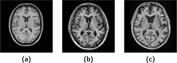
2. Differences in acquisition parameters. Even for the same pulse sequence, slight differences in acquisition parameters will yield a contrast difference. As shown in Fig. 1 (a)–(c), the three MPRAGE images were acquired using different parameters, and consequently have a different appearance.

3. Scanner differences. Variations in field strength, hardware components, manufacturer, software including reconstruction algorithms, and calibration (American College of Radiology, 2018) can have substantial impacts on the appearance of images.

Fig. 1.

(a)–(c) are ${\text{T}}_1-\text{w}$ MPRAGE images with different acquisition parameters.

The contrast variation from site to site makes it difficult for computer-assisted algorithms to provide consistent results in multi-site studies (Remedios et al., 2020). For example, a machine learning (ML) model trained on MPRAGE images from Site $A$ is likely to fail on SPGR images from Site $B$. This can be formalized as a domain shift problem, where training images $x_{\text{train}}\in {𝓧}_A$ and testing images $x_{\text{test}}\in {𝓧}_B$ acquired at Sites $A$ and $B$ are from two different domains ${𝓧}_A$ and ${𝓧}_B$. It is worth noting that “domain ” does not exclusively mean “site ” or even “scanner ”. ${\text{T}}_1-\text{w}$ images acquired from different sites are readily understood as coming from different domains. In this work, we also consider ${\text{T}}_1-\text{w}$ and ${\text{T}}_2-\text{w}$ images acquired from the same site to be from different domains. ¹

To address the domain shift problem, two broad categories of harmonization approaches have been proposed, namely statistical-based harmonization (Fortin et al., 2017; Garcia-Dias et al., 2020; 2020; Pomponio et al., 2020; Zhu et al., 2019) and image-level harmonization (Dewey et al., 2019; Liu et al., 2021; Zuo et al., 2021). These two types of harmonization differ fundamentally in how the data is used. Statistical-based harmonization methods focus on image derived measurements (IDMs), such as regional volumes (Zhu et al., 2019). In order to generate these IDMs, statistical-based harmonization requires another method (i.e., segmentation) (Dewey et al., 2019). Therefore, statistical-based harmonization can be viewed as a post-processing step, aimed at correcting the variations within a segmentation method caused by the domain shift. However, when the domain shift is too severe, the segmentation variations cannot be corrected by these statistical models. In this paper, we focus on image-level harmonization, of which the input and output are both images, and the goal is to reduce the pulse sequence based contrast variations prior to most other image processing. We note that artifacts such as gradient distortion are outside the scope of the proposed method and to our knowledge outside the scope of other image level harmonization methods. However, the effects of such artifacts could potentially be corrected using statistical-based harmonization.

As an image-to-image translation (IIT) technique, MR image harmonization (Dewey et al., 2018; 2019) alleviates domain shift by learning an intensity transformation $f(\cdot )$ between mismatched domains, e.g., $f_A(\cdot ):{𝓧}_A\to {𝓧}_B$. While $f(\cdot )$ manipulates image intensity, the underlying anatomy (geometry, tissue, etc.) should not be changed. MR harmonization can be performed in supervised and unsupervised ways, depending on the available training data. In supervised harmonization, the same anatomies are imaged across multiple sites as a requirement —this is known as traveling subjects or inter-site paired data. With inter-site paired data, pixel-to-pixel error is commonly used to train $f(\cdot )$, e.g., ${\Vert x_B-f_A\left(x_A\right)\Vert }_2$, where $x_A$ and $x_B$ are images from domains ${𝓧}_A$ and ${𝓧}_B$, respectively. Recent work by Dewey et al. (2018, 2019) proposed a supervised harmonization approach that translates an MR image across sites with only a small number of traveling subjects. The inter-site paired data aspect of supervised harmonization is a serious limitation to its use, as acquiring inter-site paired data for large numbers of sites is time-consuming, expensive, and logistically untenable. Moreover, supervised harmonization lacks generalizability as the harmonization is limited to the sites used for training.

On the other hand, unsupervised harmonization does not need inter-site paired images. Mathematically, the goal is to approximate the joint distribution $p\left(x_A,x_B\right)$ from marginal distributions $p\left(x_A\right)$ and $p\left(x_B\right)$ of domains ${𝓧}_A$ and ${𝓧}_B$. There are three main challenges in unsupervised harmonization. First, the absence of inter-site paired images means pixel-to-pixel error cannot be easily calculated. In general, deep learning (DL) based harmonization relies on domain-specific models to translate images across different domains. For example, CycleGAN (Zhu et al., 2017) translates images from domains ${𝓧}_A$ to ${𝓧}_B$ by learning a translation model $f_A(\cdot ):{𝓧}_A\to {𝓧}_B$ and a discriminator $D_B(\cdot ):{𝓧}_B\to ℝ$, mean-while, an inverse translation model $f_B(\cdot ):{𝓧}_B\to {𝓧}_A$ and a counter-domain discriminator $D_A(\cdot ):{𝓧}_A\to ℝ$ are learned jointly. Since the harmonization performance heavily depends on the discriminators’ “judgement ”, geometry shift is a common drawback of DL based unsupervised harmonization methods. Second, due to the use of domain-specific models (e.g., discriminators), current harmonization approaches do not scale well in multi-site imaging; CycleGAN (Zhu et al., 2017) needs $O\left(N^2\right)$ intensity transformation models and $N$ discriminators in an $N$-site harmonization task. We note that some works such as StarGAN (Choi et al., 2018) have a unified structure but lack interpretability in the learned features, which makes it difficult to understand the model’s behavior. Third, according to coupling theory (Lindvall, 2002), there are infinitely many possible joint distributions given two marginal distributions. Therefore, further constraints are needed to reduce the number of possible solutions. Cycle consistency is a commonly assumed constraint in unsupervised harmonization. UFDN (Liu et al., 2018), CycleGAN (Zhu et al., 2017), and UNIT (Liu et al., 2017) assume an identity transformation after applying a forward and an inverse transformation, i.e., $I=f_A\left(f_B(\cdot )\right)=f_B\left(f_A(\cdot )\right)$. Unfortunately, there is no theoretical guarantee that these additional constraints lead to a meaningful and unique solution (Cohen et al., 2018; Liu et al., 2017).

In addition to the three challenges in unsupervised harmonization, most existing harmonization works do not perform well on previously unseen sites. This means that harmonization, which is designed to alleviate domain shift in downstream tasks, suffers from domain shift it-self. When there is a new site involved, a re-training that includes images from both previous sites and the new site is typically required. This could potentially limit the applicability of those harmonization methods as transferring data across sites in medical imaging is often restricted. Fortunately, the recent development of unsupervised domain adaptation (UDA) enables DL models to adjust to unseen domains during testing. In general, a UDA model learns from a source domain with labeled data then applies itself to a target testing domain with unlabeled data (He et al., 2020b; Kamnitsas et al., 2017; Saito et al., 2018; Varsavsky et al., 2020). In IIT, an intensity translation model learns to map image data across domains; to extend this, UDA allows a pre-trained model to adjust itself to previously unseen testing domains without access to the training data used to train the original model. He et al. (2020b, 2021) used a feature autoencoder trained in the source domain as a detector of domain shift, assuming the feature autoencoder will produce low reconstruction error on the source domain data and high reconstruction error in the new domain. Thus, at test time, the reconstruction error produced by the autoencoder guides the model to adjust its parameters until the reconstruction error falls below a threshold.

Jog et al. (2015) proposed a model-based approach to address MR harmonization that generates synthetic inter-site paired images to train $f(\cdot )$. The approach assumed knowledge of the true ${\text{T}}_1$, ${\text{T}}_2$, and proton density (PD) maps of a set of atlas images, where ${\text{T}}_1$ and ${\text{T}}_2$ represent the longitudinal relaxation time and transverse relaxation time, respectively. The model first estimates acquisition parameters (e.g., echo time, flip angle, etc.) using prior knowledge of the imaging equation, then applies the estimated acquisition parameters to the atlas maps to generate synthetic inter-site paired images for harmonization. However, estimating the true acquisition parameters can be challenging and inaccurate. Additionally, the approach depends on random forests which can be significantly improved upon with current DL methods. In recent years, researchers have explored DL based disentangled representation learning approaches in medical imaging (Chartsias et al., 2019; Ouyang et al., 2021), aiming at disentangling anatomical and contrast information from medical images. Recently, Dewey et al. (2020) proposed an unsupervised MR harmonization approach which “disentangles ” the anatomical and contrast representations from the input MR images. It can harmonize MR images across sites by combining the anatomical representation from the source site with the contrast representation from the target site. However, as we discuss in Section 2.2, this approach could end up learning a locally disentangled latent space that fails to perform multi-site harmonization. We show that by incorporating information bottleneck theory (Tishby et al., 1999), we can improve upon this work and build a universal latent space of anatomy and contrast information through better disentanglement.

Based on existing work (Dewey et al., 2020; Zuo et al., 2021), we propose an unsupervised harmonization approach, CALAMITI (Contrast Anatomy Learning and Analysis for MR Intensity Translation and Integration), that overcomes common drawbacks of both supervised and unsupervised harmonization. CALAMITI does not require inter-site paired data. Instead, it takes advantage of the routinely acquired multi-contrast images of the same subject within each imaging session (called intra - site paired data). Therefore, pixel-to-pixel error can be penalized during training. Once trained, CALAMITI does not need intra-site paired images, as it is evaluated on a single image. Furthermore, CALAMITI is informed by information bottleneck theory to learn a globally disentangled latent space of anatomy and contrast information. The model has a unified structure for multi-site harmonization; thus, the model size does not grow with the number of sites. Finally, CALAMITI contains certain aspects of UDA approaches and is able to adapt itself to a new testing site using a straightforward fine-tuning. We evaluated CALAMITI using a variety of datasets including the Baltimore Longitudinal Study of Aging (BLSA) dataset (Resnick et al., 2000; Thambisetty et al., 2010) as well as the publicly available IXI ² and OASIS3 (LaMontagne et al., 2019) datasets to show its broad applicability. Both qualitative and quantitative results show that the proposed method achieves superior performance in harmonization compared to other unsupervised MR harmonization approaches. In addition to the aforementioned contributions to harmonization, we also propose a fusion network to achieve better slice-to-slice consistency in harmonized images. Our approach yields a statistically significant improvement in the consistency of brain structure segmentation in multi-site imaging. Furthermore, we demonstrate how the contrast latent space, arising from disentanglement, can be used beyond harmonization.

2. Method

2.1. The disentangling framework

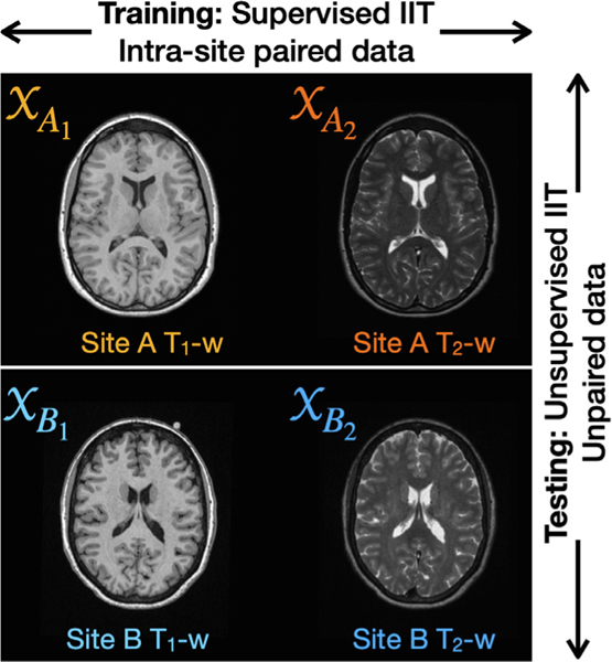
CALAMITI uses intra-site paired MR images from multiple sites for model training. Specifically, ${\text{T}}_1-\text{w}$ and ${\text{T}}_2-\text{w}$ images of the same subject are used to do paired ${\text{T}}_1$-to-${\text{T}}_2$ synthesis (Roy et al., 2013; Zuo et al., 2020)—i.e., supervised IIT —within each site. Here, we emphasize the relationship between “site ”, “domain ”, and “MR contrast ”. Given Sites $A$ and $B$ in training, there are four domains ${𝓧}_{A_1}$, ${𝓧}_{A_2}$, ${𝓧}_{B_1}$, and ${𝓧}_{B_2}$ (shown in Fig. 2), where an alphabetical index denotes the site (Site $A$ or $B$) and a numerical index denotes the different contrasts (${\text{T}}_1-\text{w}$ and ${\text{T}}_2-\text{w}$, respectively). Since the model is trained to do supervised IIT within each site, no extra constraints (e.g., cycle consistency) are needed, and pixel-to-pixel accuracy can be used to avoid the geometry shift problem.

Fig. 2.

Given ${\text{T}}_1-\text{w}$ and ${\text{T}}_2-\text{w}$ images from Sites $A$ and $B$, there are four domains ${𝓧}_{A_1}$, ${𝓧}_{A_2}$, ${𝓧}_{B_1}$, and ${𝓧}_{B_2}$, where an alphabetical index denotes the site (Site $A$ or $B$) and a numerical index denotes the different contrasts (${\text{T}}_1-\text{w}$ and ${\text{T}}_2-\text{w}$, respectively). Our method learns from supervised image-to-image translation within each site during training, and at test time can do cross-site unsupervised image-to-image translation.

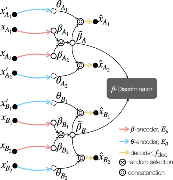
The proposed framework is shown in Fig. 3. It has an anatomical encoder ($E_{\beta }$), a contrast encoder ($E_{\theta }$), a decoder ($f_{\text{dec}}$), and a $\beta$-discriminator ($D_{\beta }$). We show the role of each network component in this section and the implication of $D_{\beta }$ in Section 2.2. During training, $E_{\beta }$ and $E_{\theta }$ extract anatomical ($\beta$) and contrast information ($\theta$), respectively, from input images $x$ and $x^{\prime }$. The images $x$ and $x^{\prime }$ share the same contrast, but cover different portions of the anatomy. This training strategy prevents the contrast representation $\theta$ from capturing anatomical information, and is achieved by selecting different slices of the same volume. The learned contrast representation $\theta$ is a vector with a much lower dimension than $x^{\prime }$. In CALAMITI, we assume $x=f_{\text{dec}}(\theta ,\beta )$, which means that the decoder $f_{\text{dec}}(\cdot ,\cdot )$ needs two pieces of information, $\theta$ and $\beta$, to generate a synthetic image. Since $\beta$ is forced to capture the common information (which is anatomy) between ${\text{T}}_1-\text{w}$ and ${\text{T}}_2-\text{w}$ images, $f_{\text{dec}}(\cdot ,\cdot )$ seeks contrast information from $\theta$. Since the only “useful ” information in $x^{\prime }$ to synthesize $x$ is the common contrast, we would expect $\theta$ to learn contrast information during training. To prevent $\beta$ from capturing contrast information, we implemented the same approach as (Dewey et al., 2020; Liu et al., 2020), where $\beta$ is a one-hot encoded multi-channel image generated by a Gumbel-softmax layer. As mentioned in (Chartsias et al., 2019), the one-hot encoding restricts the capacity of $\beta$; this, in conjunction with our training scheme, promotes only essential anatomical information being captured in $\beta$.

Fig. 3.

High-level framework of the proposed method. Colored arrows indicate network components. Dots, dashed circles, and solid circles represent images, $\theta$’s, and $\beta$’s, respectively.

Within each site (e.g., Site $A$), since $x_{A_1}$ and $x_{A_2}$ share the same anatomy, we want the learned anatomical representations ${\beta }_{A_1}$ and ${\beta }_{A_2}$ to be the same. We encourage this $\beta$ similarity during training in two ways. First, we employ a $\beta$ similarity loss (${𝓛}_{\beta }$) between the two $\beta$’s and, second, we implement a random selection process between ${\beta }_{A_1}$ and ${\beta }_{A_2}$ before decoding. The random selection operator makes a choice between ${\beta }_{A_1}$ and ${\beta }_{A_2}$ for each $\beta$ channel. The one-hot encoding, the $\beta$ similarity loss, and the random $\beta$ swapping, taken together, discourage $\beta$ from capturing undesired contrast information from the input images. Before decoding, the $\theta$ vector is broadcast to have the same height and width as the $\beta$ map. The broadcast $\theta$ is then concatenated with the randomly selected $\tilde{\beta }$ in the channel dimension, where $\tilde{\beta }$ is the anatomical representation after random selection. The concatenated variable is then sent to the decoder, $f_{\text{dec}}$, and the value of $\theta$ determines the contrast of the synthetic images. It is important to note that the same encoder and decoder networks are applied to all the sites. After the model is trained, cross-site harmonization can be achieved by combining a $\beta$ from a source site with a $\theta$ from a target site.

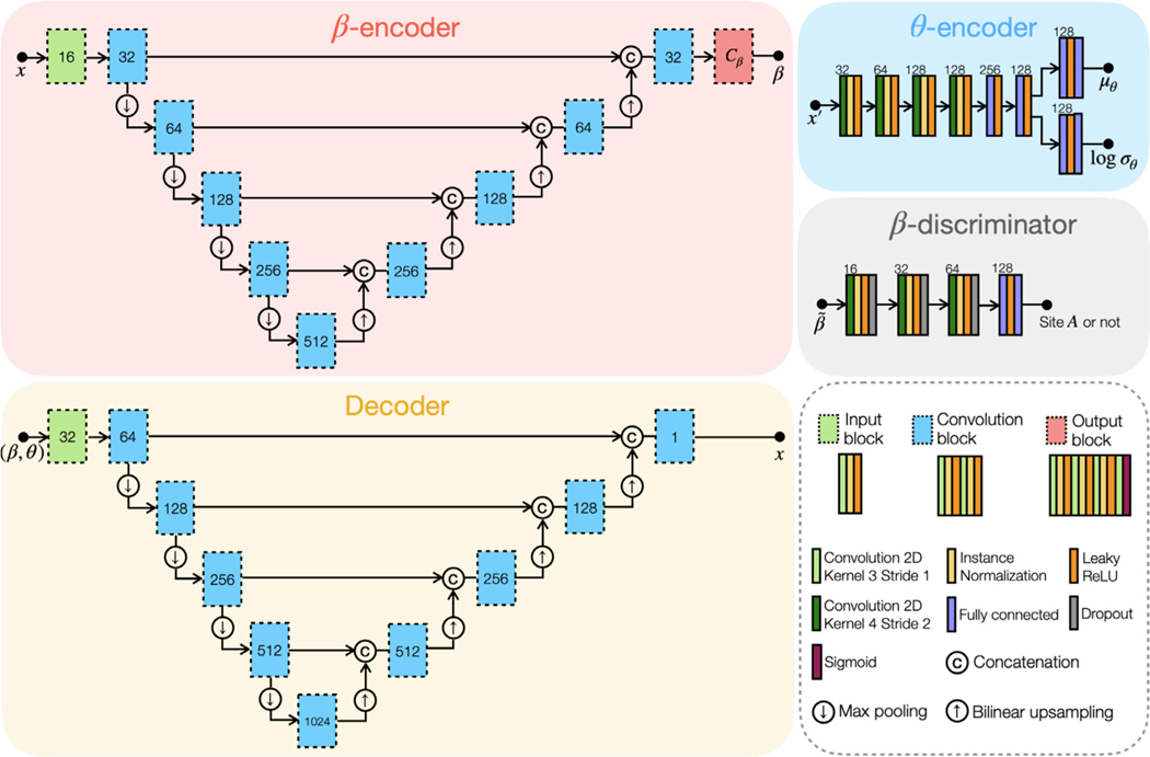
The architectures of the networks in CALAMITI are shown in Fig. 4. $E_{\beta }$ has a U-Net (Ronneberger et al., 2015) structure with four levels. $f_{\text{dec}}$ has a similar architecture as $E_{\beta }$, with the exception that $f_{\text{dec}}$ does not have an output block and the number of channels of the remaining blocks is doubled. Like the variational autoencoder in Kingma and Welling (2013), $\theta$ is assumed to have a Gaussian distribution with learnable mean and standard deviations, i.e., $\theta \sim 𝓝\left({\mu }_{\theta },{\sigma }_{\theta }I\right)$. Therefore, $E_{\theta }$ takes an input MR image $x^{\prime }$ and produces ${\mu }_{\theta }$ and log ${\sigma }_{\theta }$ as outputs. Our $\beta$-discriminator, $D_{\beta }$, is a one-class discriminator that classifies whether an input $\beta$ is from Site $A$ or not. Therefore, the number of output channels of $D_{\beta }$ is 1. Details and implications of our $\beta$-discriminator, $D_{\beta }$, are described in Section 2.2.

Fig. 4.

Network architecture of the proposed method. Numbers next to each box indicate the number of output feature channels. $C_{\beta }$ indicates the number of $\beta$ channels.

2.2. Learning a global anatomical space

Since training is conducted by doing supervised IIT within each site, it is possible that, without coordination, $E_{\beta }$ will learn a distinct $\beta$ space for each site. We refer to a site-specific $\beta$ space as a locally disentangled $\beta$ space. In this case, combining $\beta$ and $\theta$ from different sites would be non-ideal. To avoid this, we want to encourage $E_{\beta }$ to learn a consistent anatomical representation across sites. In other words, $\beta$ and $\theta$ should be globally disentangled, which leads to our use of a discriminator $D_{\beta }$ applied to the $\beta$ spaces. The goal of the discriminator is to identify whether $\beta$ captures site-specific information and it is implemented as a one-class discriminator that classifies whether an input $\beta$ is from Site $A$ or not. In Section 3.2, we show that $D_{\beta }$ also enables our model to adapt itself to a new testing site. We also tried using a multi-class $\beta$-discriminator that classifies the site index directly. However, this approach does not permit domain adaptation and, also, its performance is not significantly different from the one-class $D_{\beta }$. Thus, in the remainder of the paper we focus exclusively on the one-class discriminator $D_{\beta }$.

Our $\beta$-encoder, $E_{\beta }$, tries to “fool ” $D_{\beta }$ by providing similarly distributed $\beta$’s across sites. In this way, our $E_{\beta }$ and $D_{\beta }$ together form an adversarial training scheme on the latent space $\beta$. The minimax training goal between $E_{\beta }$ and $D_{\beta }$ is given by

$$\underset{E_{\beta }}{\min }\underset{D_{\beta }}{\max }{\mathbb{E}}_{x_A}\left[\log D_{\beta }\left(E_{\beta }\left(x_A\right)\right)\right]+{\mathbb{E}}_{x_{\overline{A}}}\left[\log \left(1-D_{\beta }\left(E_{\beta }\left(x_{\overline{A}}\right)\right)\right)\right],$$ (1)

where the subscript $\overline{A}$ denotes MR images or anatomical representations from sites other than Site $A$. Accordingly, the loss functions of $D_{\beta }$ and $E_{\beta }$ are defined as

$${𝓛}_{D_{\beta }}=-{\mathbb{E}}_{{\beta }_A}\left[\log D_{\beta }\left({\beta }_A\right)\right]-{\mathbb{E}}_{{\beta }_{\overline{A}}}\left[\log \left(1-D_{\beta }\left({\beta }_{\overline{A}}\right)\right)\right]$$ (2)

$${𝓛}_{E_{\beta }}={\mathbb{E}}_{x_A}\left[\log D_{\beta }\left(E_{\beta }\left(x_A\right)\right)\right]+{\mathbb{E}}_{x_{\overline{A}}}\left[\log \left(1-D_{\beta }\left(E_{\beta }\left(x_{\overline{A}}\right)\right)\right)\right],$$ (3)

where $\beta =E_{\beta }(x)$.

The objective of our $D_{\beta }$ is different from traditional IIT methods. In other unsupervised IIT methods, such as CycleGAN (Zhu et al., 2017) and UNIT (Liu et al., 2017), discriminators typically function on the image space. In our proposed method, $D_{\beta }$ is a latent space discriminator, which has several advantages. First, our unified network structure including $D_{\beta }$ means the model size remains constant when the number of sites increases. Compared with CycleGAN (Zhu et al., 2017), which needs dedicated site-wise generators and discriminators, CALAMITI offers a significant saving on the number of parameters —potentially enabling an infinite number of sites to be used within the framework. Second, CALAMITI is based on the assumption that an observed MR image is a function of the underlying anatomy ($\beta$) and imaging parameters ($\theta$). Regularizing the $\beta$ space instead of the image space helps our decoder $f_{\text{dec}}$ act like a universal imaging equation that generalizes to various anatomies and contrasts. Third, as we show in Section 2.4, the one-class configuration of $D_{\beta }$ enables our model to adapt itself to a new testing site with a fine-tuning on just a subset of the testing site images (without any data from the original training sites). Table 1 provides a summary comparison of multiple unsupervised IIT methods, noting the capabilities of the proposed work in comparison to previous works.

Table 1.

Features of recent unsupervised IIT and UDA approaches that can be used to do MR harmonization.

	Bidirectional Translation	Multiple Domains	Unified Structure	Disentangling	Global Latent Space	Domain Adaptation
CycleGAN (Zhu et al., 2017)	√	-	-	-	-	-
StarGAN (Choi et al., 2018)	√	√	√	-	-	-
UNIT (Liu et al., 2017)	√	-	-	√	-	-
MUNIT (Huang et al., 2018)	√	√	-	√	-	-
DCMIT (Xia et al., 2020)	√	√	-	√	√	-
SDA-net (He et al., 2020b)	-	-	√	-	-	√
Moyer et al. (Moyer et al., 2020)	√	√	√	-	-	-
Dewey et al. (Dewey et al., 2020)	√	√	√	√	-	-
CALAMITI (ours)	√	√	√	√	√	√

2.3. Information bottleneck and disentangling

In our network structure, $E_{\theta }$, $E_{\beta }$, and $f_{\text{dec}}$ form a conditional variational autoencoder (CVAE) (Sohn et al., 2015) in which $\beta$ acts as a condition and $\theta$ is the bottleneck latent variable. Compared with the original CVAE structure in Sohn et al. (2015), the major difference is that the condition variable $\beta$ is not connected to the CVAE encoder $E_{\theta }$. In this section, we show that our network structure is a special case of the CVAE due to the disentangling objective, and our model can be understood as solving a conditional information bottleneck problem.

Information bottleneck (IB) theory, originally proposed by Tishby et al. (1999), aims at learning compressed representations by solving a constrained optimization problem. In IB theory, there is an input variable $X$ (e.g., MR image) and a task variable $Y$ (e.g., a classification label), and the goal is to learn a latent representation $Z$, such that $Z$ captures the maximal information about the task $Y$ and minimal information about the input $X$, i.e.,

$$Z^{\ast }=\underset{Z}{\arg \min }I(X;Z)-\lambda I(Y;Z),$$ (4)

where $I(\cdot ;\cdot )$ denotes mutual information, and $\lambda$ is a hyperparameter. In recent years, IB theory has been used in understanding neural networks’ behavior and disentangled representation learning (Dai et al., 2018).

Theorem 1.

It can be shown that optimizing the proposed network structure is equivalent to solving a conditional information bottleneck problem, i.e.,

$${\theta }^{\ast }=\underset{\theta }{\arg \min }I\left(X^{\prime };\theta \right)-\lambda I(X;\theta \mid \tilde{\beta }).$$ (5)

The proof of Theorem 1 is provided in Appendix A. An intuitive understanding of Eq. (5) is that we would like to learn a compressed representation $\theta$, such that $\theta$ carries minimum information about the input image $X^{\prime }$, while the conditional mutual information between $\theta$ and the target image $X$ is maximized. Since the only common information between $X$ and $X^{\prime }$ is contrast, we would expect $\theta$ to capture contrast information after training.

Eq. (5) can be re-organized as a Kullback–Leibler (KL) divergence term and a reconstruction term, and optimized directly as follows

$${\theta }^{\ast }=\underset{\theta }{\arg \min }{𝓓}_{\text{KL}}\left[p\left(\theta \mid x^{\prime }\right)\left|\right|p(\theta )\right]-\lambda {\mathbb{E}}_{p\left(\theta \mid x^{\prime }\right)}[\log p(x\mid \theta ,\tilde{\beta })],$$ (6)

where $p(\theta )$ is assumed to be $𝓝(0,I)$. $p\left(\theta \mid x^{\prime }\right)$ and $p(x\mid \theta ,\tilde{\beta })$ can be modeled using a probabilistic encoder ($E_{\theta }$) and decoder ($f_{\text{dec}}$), respectively. Since both $p\left(\theta \mid x^{\prime }\right)$ and $p(\theta )$ are assumed to be Gaussian distributed, there is a closed-form| solution to the KL divergence term, and the expectation term in Eq. (6) is estimated using $l_1$ loss. It is worth mentioning that we could also use $\theta$ as a condition variable and $\beta$ as the latent bottleneck variable of the CVAE. However, in that case, calculating

$${𝓓}_{\text{KL}}[p(\beta \mid x)\parallel p(\tilde{\beta })]$$

for categorical distributions —the one-hot encoded $\beta$ follows a categorical distribution —would be difficult.

The loss function for training $D_{\beta }$ is given by Eq. (2). It follows from Eq. (6) and the assumptions about $p\left(\theta \mid x^{\prime }\right)$ and $p(x\mid \theta ,\tilde{\beta })$ that the loss function for the other network components (i.e., $E_{\beta }$, $E_{\theta }$, and $f_{\text{dec}}$) includes two reconstruction terms ($l_1$ and perceptual (Johnson et al., 2016) losses), a KL divergence term, a $\beta$ similarity loss ($l_1$), and an adversarial loss for $E_{\beta }$, i.e.,

$$\begin{gathered} 𝓛={\lambda }_1|\widehat{x}-x{|}_1+{\lambda }_2|\text{VGG}(\widehat{x})-\text{VGG}(x){|}_1 \\ +{\lambda }_3{𝓓}_{\text{KL}}\left[p\left(\theta \mid x^{\prime }\right)\parallel p(\theta )\right] \\ +{\lambda }_4{\left|{\beta }_1-{\beta }_2\right|}_1+{\lambda }_5{𝓛}_{E_{\beta }}, \end{gathered}$$

where ${𝓛}_{E_{\beta }}$ is the adversarial loss for the $\beta$-encoder given in Eq. (3). ${\left|\text{VGG}(\widehat{x})-\text{VGG}(x)\right|}_1$ calculates the perceptual loss (Johnson et al., 2016) between $\widehat{x}$ and $x$ and ${\lambda }_i$, $i=1,\dots ,5$, are hyperparameters. According to our experiments, we found that our model is not very sensitive to the choice of hyperparameters. Except for the KL divergence and the perceptual loss, the other losses are weighted to achieve a similar magnitude as the $l_1$ reconstruction loss. We also conducted an ablation study, which we show in Section 3.2, to explore the usefulness of the perceptual loss.

2.4. Domain adaptation

When a pre-trained ML model is applied to a testing domain that is different than the training domain, a retraining that includes data pools from both previous and new domains is often required. However, for medical images, training and testing data are likely to come from different sources, and data sharing is often restricted. So we ask the question: how can we adapt our algorithm to a new domain when we do not have access to any of the original training data? It turns out that, because of its design, CALAMITI can be adapted to a new testing domain by applying fine-tuning using just a small subset of the testing domain images.

Specifically, suppose CALAMITI was previously trained on Sites $A$ and $B$ and then we want to apply the network to data from Site $C$. To do this, we use a subset of images from Site $C$ and carry out regular training —i.e., supervised IIT within Site $C$—except that only the output block of $E_{\beta }$ and the fully connected layers of $E_{\theta }$ (see Fig. 4) are allowed to be updated. Intuitively, this fine-tuning procedure produces a local $\beta$ space for Site $C$, since Sites $A$ and $B$ are not involved. However, since our $D_B$ is trained to decide whether an input $\tilde{\beta }$ is from Site $A$ or not, and it is fixed during fine-tuning, $D_B$ will produce a high cost for $E_{\beta }$ until the newly learned ${\tilde{\beta }}_C$ matches the distribution of the $\beta$’s from Site $A$. After this fine tuning, harmonization from Site $C$ to Site $A$ can be done by first calculating ${\beta }_C$ on a given image from Site $C$ using the fine-tuned $\beta$-encoder, $E_{\beta }^{\prime }$, and replacing the computed ${\theta }_C$ with an average ${\theta }_A$ as input to the decoder. In fact, data from Site $C$ can be harmonized to any site included in the original training by replacing its computed ${\theta }_C$ with a desired $\theta$ value.

2.5. 3D fusion network

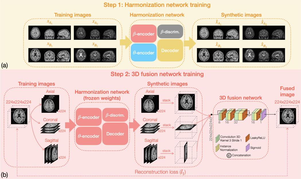
Due to limited GPU capacity, CALAMITI harmonizes images in 2D. In order to achieve better slice consistency, we propose a fusion network that combines multiple harmonized 2D slices into a single 3D volume. The fusion network is trained after the harmonization network. As shown in Fig. 5 (a), Step 1 is the training of the harmonization network using a pool of multi-site multi-orientation 2D slices ($x^{\prime }$ are also used in training the harmonization network but not shown here. See Fig. 3 for more details.). Note that for each 3D volume, only the center 80 axial slices, 100 coronal slices, and 100 sagittal slices are used in training. In Step 2, the weights of the harmonization network are frozen to train the 3D fusion network. As shown in Fig. 5 (b), the data to train the 3D fusion network are the same as those used to train the harmonization network. However, this time each 3D volume is decomposed into axial, coronal, and sagittal slices, and all slices are then sent to the pre-trained harmonization network to generate a set of synthetic 2D images. After-wards, 2D synthetic images of the three orientations are stacked into three volumes. The three stacked synthetic volume images are then sent to the fusion network to create a final fused image. Meanwhile, an $l_1$ reconstruction loss is calculated between the fused image and the original 3D image to train the fusion network. In contrast to the harmonization network, we train separate fusion networks for ${\text{T}}_1-\text{w}$ and ${\text{T}}_2-\text{w}$ images. However, for each contrast our fusion network has a unified structure design for all sites. We note that there are other ways to combine 2D slices into 3D volumes. In (Dewey et al., 2018; 2019), instead of using a fusion network to combine the three stacked 3D volumes, researchers used the median value calculated at each voxel as the intensity value of the final fused image. Detailed comparison between the median filter approach and the proposed fusion approach is provided in Section 3.2.

Fig. 5.

Training the pseudo 3D implementation includes two parts: (a) the harmonization network is first trained using a pool of multi-site multi-orientation MR slices. Then (b) weights of the harmonization network are frozen to train the 3D fusion network. The fusion network learns to combine the three stacked volume images into one single fused image.

3. Experiments

3.1. Materials and data preprocessing

Three MR datasets acquired from 10 sites (scanners) are used to evaluate the proposed harmonization method. Specifically, there are two sites from the IXI brain dataset (Sites $A$ and $B$), four sites from the OASIS3 dataset (LaMontagne et al., 2019) (Sites $C$ thru $F$), and four sites from the BLSA dataset (Resnick et al., 2000; Thambisetty et al., 2010) (Sites $G$ thru $J$). Scanner information is provided in Table 2. All subjects used in this study are healthy controls. In the OASIS3 dataset, there are longitudinal scans with small intervals between the two visits; MR images from both visits are held out as traveling subjects for quantitative evaluation. In particular, for Sites $C$ and $D$, there are 10 traveling subjects with a gap between scans of 162 ± 72 days, and for Sites $E$ and $F$, there are 10 subjects with a gap between scans of 13 ± 5 days.

Table 2.

Scanner information, sequence name with imaging parameters (TE, TR, and TI if known), acquisition resolution, and age information (mean ± standard deviation) of the training and evaluation datasets.

	Site $A$ (IXI)	Site $B$ (IXI)	Site $C$ (OASIS3)	Site $D$ (OASIS3)	Site $E$ (OASIS3)
	Philips Intera 1.5T	Philips Gyroscan 3T	Siemens Sonata 1.5T	Siemens TimTrio 3.0T	Siemens TimTrio 3.0T
	Age: 44.5 ± 7.8	Age: 52.l ± 9.2	Age: 60.4 ± 7.1	Age: 65.5 ± 10.5	Age: 58.2 ± 9.3
${\text{T}}_1-\text{w}$	MPRAGE: 4.6ms, unknown, unknown	MPRAGE: 4.6ms, unknown, unknown	MPRAGE: 3.93ms, 1.9s, 1.1s	MPRAGE: 3.16ms, 2.4s, 1s	MPRAGE: 3.16ms, 2.4s, 1s
	1.2 × 0.94 × 0. 94mm	1.2 × 0.94 × 0.94mm	1 × 1 × 1mm	1 × 1 × 1mm	1 × 1 × 1mm
${\text{T}}_2-\text{w}$	TSE: 100ms, 8.2s	TSE: 100ms, 8.2s	TSE: 116ms, 6.0s	TSE: 455ms, 3.2s	TSE: 455ms, 3.2s
	0.94 × 0.94 × 1.25mm	0.94 ×0.94 × 1.25mm	0.9 × 0.9 × 5mm	1 × 1 × 1mm	1 × 1 × 1mm
	Site $F$ (OASIS3)	Site $G$ (BLSA)	Site $H$ (BLSA)	Site $I$ (BLSA)	Site $J$ (BLSA)
	Siemens BioGraph 3.0T	Philips Intera 1.5T	Philips Achieva 3T	Philips Achieva 3T	Philips Achieva 3T
	Age: 68.2 ± 6.9	Age: 71.2 ± 10.9	Age: 69.3 ± 7.9	Age: 79.5 ± 11.1	Age: 78.4 ± l2.2
${\text{T}}_1-\text{w}$	MPRAGE: 2.95ms, 2.3s, 0.9s	MPRAGE: 3.3ms, 3s, unknown	MPRAGE: 3.1ms, 3s, 0.8s	MPRAGE: 3.1ms, 3s, 0.8s	MPRAGE: 3.1ms, 3s, 0.8s
	1.05 × 1.05 × 1.2mm	0.94 × 0.94 × 1.5mm	1 × 1 × 12mm	1 × 1 × 12mm	1.2 × 1 × 1mm
${\text{T}}_2-\text{w}$	TSE: 454ms, 3.2s	TSE: 100ms, 5.0s	TSE: 100ms, 3.0s	TSE: 100ms, 3.0s	TSE: 100ms, 3.0s
	1 × l × 1mm	0.94 × 0.94 × 3mm	0.94 × 0.94 × 3mm	0.94 × 0.94 × 3mm	0.94 × 0.94 × 3mm

The data preprocessing steps include N4 inhomogeneity correction (Tustison et al., 2010), super-resolution (Zhao et al., 2020) for 2D acquired scans, registration to 1mm³ MNI space, and white matter peak normalization (Reinhold et al., 2019). After preprocessing, each volume has spatial dimension of 224 × 192 × 192. Each volume image is then zero-padded to 224 × 224 × 224 to guarantee that the multi-orientation slices used in training have the same dimensions. We used 10 subjects from each site to train both the harmonization network and the fusion network. In our implementation, our batch size is 8, and the optimizer is Adam. Our evaluations were separately conducted on multiple varieties of GPUs, including an Nvidia Quadro RTX 8000 (48 GB memory) and an Nvidia Tesla M40 (24 GB memory).

3.2. Qualitative and quantitative evaluation

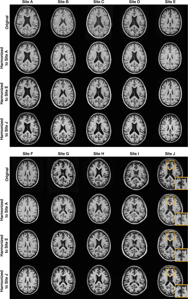
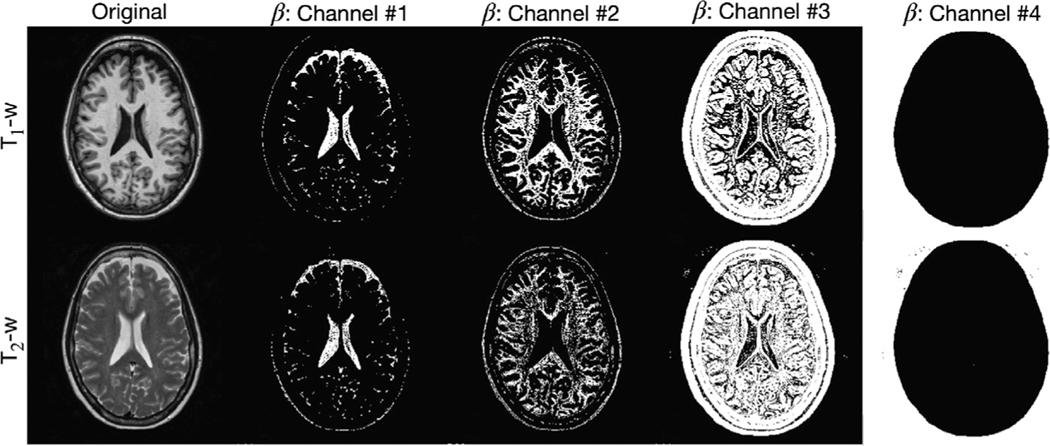
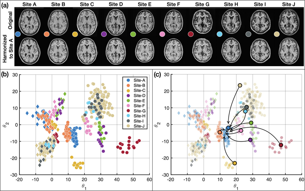
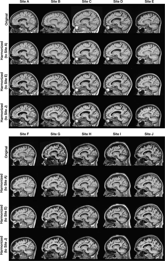
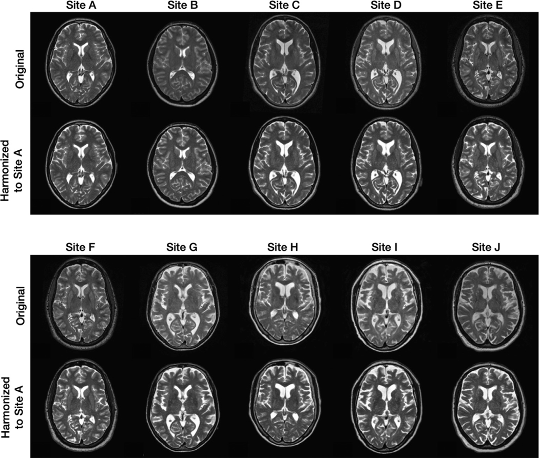
In this experiment, we chose $\theta$ to be a two-dimensional vector and $\beta$ to be a four-channel one-hot encoded image. These values were chosen empirically after some experimentation. Fig. 6 provides examples from our 10-site harmonization experiment. ${\text{T}}_1-\text{w}$ images are harmonized to each of Sites $A$, $E$, and $J$. The contrast change after harmonization can better be visualized in the GM, WM, and adipose. For example, the GM and WM contrast decreases after harmonizing the MR image of Site $J$ to Site $A$, as highlighted by the yellow boxes. Harmonized images of the same subjects from a sagittal view are provided in Appendix B. Unless stated otherwise all the results of CALAMITI are generated using the 3D implementation described in Section 2.5. Our experiments have focused on the ${\text{T}}_1-\text{w}$ images. With regard to the ${\text{T}}_2-\text{w}$ images, we achieve similar image quality as the ${\text{T}}_1-\text{w}$ images. In Appendix C, we provide a visualization of ${\text{T}}_2-\text{w}$ images harmonization. Fig. 7 provides a visualization of a four-channel $\beta$ from paired ${\text{T}}_1-\text{w}$ and ${\text{T}}_2-\text{w}$ images. Interestingly, three channels of $\beta$ roughly capture CSF-like, GM-like, and WM-like structures, and the remaining channel is the background. We also notice that the $\beta$’s of the ${\text{T}}_1-\text{w}$ and ${\text{T}}_2-\text{w}$ images are not entirely identical. We view this as a limitation of the current method and we discuss this in more details in Section 4.2. Fig. 8 (b) provides a scatter plot of the $\theta$ space for all the testing images from the 10 sites. As can be seen from the figure, MR images with similar acquisition parameters are visually similar and have similar $\theta$’s whereas images acquired using different magnetic field strengths (i.e., 1.5T vs. 3T) are separated in $\theta$ space (especially for the ${\text{T}}_1-\text{w}$ images shown using the circular disk markers). For example, Sites $D$ and $E$ have identical acquisition parameters and, thus, it is re-assuring to see that the $\theta$ clusters of the two sites overlap in Fig. 8. On the other hand, the 10 held-out traveling subjects from Sites $E$ and $F$ have distinct $\theta$ clusters, despite their shared anatomies and very similar contrasts. This further supports our claim that the learned $\theta$ and $\beta$ are properly disentangled. Similar $\theta$ clustering can be observed for the ${\text{T}}_2-\text{w}$ images. Additionally, since our $D_{\beta }$ produces the same adversarial loss for $E_{\beta }$ of all non-Site $A$ images, the separation in $\theta$ space of each site is completely data-driven. In Fig. 8 (c), 10 example images from the 10 sites are harmonized to Site $A$. The harmonized images are then sent to $E_{\theta }$ to calculate a $\theta$ value. As shown in the figure, not only does the contrast of MR images becomes similar after harmonization, but the $\theta$ values are also clustered around the target $\theta$ that is used in harmonization.

Fig. 6.

Shown are the original axial orientation of ${\text{T}}_1$-weighted MR images from 10 sites and their corresponding harmonized images for Sites $A$, $E$, and $J$.

Fig. 7.

The four $\beta$-channels from a pair of ${\text{T}}_1-\text{w}$ and ${\text{T}}_2-\text{w}$ images.

Fig. 8.

(a) MR images before and after harmonization. (b) A visualization on the $\theta$-space of all the testing images (Circles: ${\text{T}}_1-\text{w}$ images; Diamonds: ${\text{T}}_2-\text{w}$ images; Colors listed denote a specific site). (c) ${\text{T}}_1-\text{w}$ images of 10 subjects selected from the 10 sites are harmonized to Site $A$ (target $\theta$ value shown in blue). The harmonized ${\text{T}}_1-\text{w}$ images are then sent to the $\theta$-encoder. The arrows indicate the change in the $\theta$ values after harmonization. (For interpretation of the references to colour in this figure legend, the reader is referred to the web version of this article.)

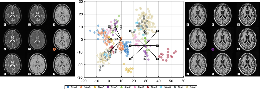
Since our networks form a CVAE and our decoder is trained to act like a “universal ” imaging equation, when we interpolate our $\theta$ space, we can generate different contrasts of MR images. As shown in Fig. 9, two groups of MR images are generated by interpolating within the $\theta$ space. On the right, a $\beta$ variable is extracted from a ${\text{T}}_1-\text{w}$ image denoted by the purple dot, then 8 different $\theta$ values combined with the extracted $\beta$ are fed into the decoder to generate corresponding synthetic MR images. An inter-site contrast transition can be observed from the 3 × 3 image grid. As $\theta$ moves from left to right, synthetic images show more GM/WM contrast. As $\theta$ moves from top to Sites $C$ and $G$, the fat tissue intensity becomes brighter, similar as the original images of Sites $C$ and $G$ (see Fig. 6). On the left of Fig. 9, a similar interpolation is explored with the focus being the transition area between the ${\text{T}}_1-\text{w}$ and ${\text{T}}_2-\text{w}$ contrasts in the $\theta$ space. There are some $\theta$ values that are located on the apparent boundary between the two contrasts. For those $\theta$’s, the contrast of the corresponding synthetic images are also between ${\text{T}}_1-\text{w}$ and ${\text{T}}_2-\text{w}$. Note that in Fig. 9 we use the median filtering approach described in (Dewey et al., 2018; 2019) to generate 3D synthetic images from 2D slices. This is because there is no real MR image with the interpolated $\theta$ value to train our fusion network.

Fig. 9.

Interpolation in $\theta$ space and the corresponding synthetic images. On the left, $\beta$ is calculated from the orange circle and nine different $\theta$ values are fed into the decoder to generate the corresponding synthetic images, highlighting the transition area between ${\text{T}}_1-\text{w}$ and ${\text{T}}_2-\text{w}$ $\theta$’s. In the center we display our 2D $\theta$ space, in which circles indicate $\theta$’s for ${\text{T}}_1-\text{w}$ images and diamonds indicate $\theta$’s for ${\text{T}}_2-\text{w}$ images, and colors correspond to sites. On the right, a $\beta$ is calculated from the center circle and nine different $\theta$ values are fed into the decoder to generate corresponding synthetic images. Synthetic images and the corresponding $\theta$ values are matched either by numerical (left sub-panel) or alphabetical (right sub-panel) indexes.

To quantitatively evaluate the proposed harmonization approach, we calculated the structural similarity index measurement (SSIM) (Wang et al., 2004) and peak signal to noise ratio (PSNR) value using the held-out traveling subjects. The SSIM between two grayscale images $x$ and $y$ is defined as

$$\text{SSIM}(x,y)=\frac{\left(2{\mu }_x{\mu }_y+c_1\right)\left(2{\sigma }_{xy}+c_2\right)}{\left({\mu }_x^2+{\mu }_y^2+c_1\right)\left({\sigma }_x^2+{\sigma }_y^2+c_2\right)},$$

where ${\mu }_x$, ${\mu }_y$, ${\sigma }_x^2$, ${\sigma }_y^2$, ${\sigma }_{xy}$ are the mean values of the images $x$ and $y$, the variance of the images $x$ and $y$, and the covariance of $x$ and $y$, respectively. $c_1$ and $c_2$ are used to stabilize the calculation. The PSNR between a 3D image $x$ and a reference image $y$ with dimensions $M\times N\times K$ is defined as

$$\text{PSNR}(x,y)=10{\log }_{10}\left(\frac{{\max }_I^2}{\text{MSE}}\right),$$

where ${\text{Max}}_I$ denotes the maximum possible intensity value of the image, and MSE denotes the mean squared error between $x$ and $y$, i.e.,

$$\text{MSE}(x,y)=\frac{1}{MNK}\sum _{m=1}^M\sum _{n=1}^N\sum _{k=1}^K{[x(m,n,k)-y(m,n,k)]}^2.$$

In Table 3, we show these quantities for CALAMITI and three other unsupervised harmonization approaches: 3D histogram matching (Hist), CycleGAN (Zhu et al., 2017), and Dewey et al. (2020). To investigate the usefulness of the perceptual loss and the proposed 3D fusion network, we also conducted an ablation study. Both SSIM and PSNR were calculated on 3D volumes. Note that although CALAMITI supports a pseudo 3D implementation, both CycleGAN and Dewey et al. methods are built on 2D. To provide a direct and fair comparison, we use the same strategy proposed in Dewey et al. (2018, 2019), where the authors use three-orientation 2D slices in model training, and stack slices from axial, coronal, and sagittal views to obtain three 3D volumes. The three volumes are then combined into one by calculating the median value of each voxel, we denote this by “median ”. We report results of CALAMITI using both “median ” and the proposed 3D fusion network (which we denote as “fusion ”). We also report the results of CALAMITI with and without the perceptual loss in training. Paired Wilcoxon signed rank tests were conducted between the default CALAMITI (perceptual and fusion) and the remaining comparison methods, including no harmonization (“no har ”). Except for the measurements indicated by †, the proposed method achieves significant improvements ($p<.05$, $N=10$) over the comparison methods (In this comparison, the null hypothesis is that the difference in SSIM or PSNR between the two methods has a zero median.)

Table 3.

Quantitative evaluation of several unsupervised harmonization methods and an ablation of the proposed method using the held-out traveling subjects. Both SSIM and PSNR are computed on 3D volumes, and they are reported as “mean ”± “standard deviation ”.“median ” denotes the 2D-to-3D median fusing approach similar to Dewey et al. (2019). “fusion ” indicates our proposed 2D-to-3D fusing method described in Section 2.5. The proposed method shows significant improvements ($p<.05$, $N=10$) over all comparison methods based on paired Wilcoxon signed rank tests, with exceptions labeled by ^†. Bold numbers indicate the best mean performance.

	Combine	Perceptual		Site $C\to D$		Site $D\to C$		Site $E\to F$		Site $F\to E$
No har	–	–	SSIM	0.7647	±0.0151	0.7647	±0.0151	0.8517	±0.0343	0.8517	±0.0343†
			PSNR	25.62	±0.85	25.62	±0.85	27.86	±1.24	27.86	±1.24
Hist	–	–	SSIM	0.7293	±0.0368	0.8090	±0.0374	0.8248	±0.0529	0.8014	±0.0786
			PSNR	25.99	±0.47	27.86	±0.53	26.40	±1.89	27.20	±2.41
CycleGAN	median	–	SSIM	0.7975	±0.0208	0.8286	±0.0100	0.8257	±0.0202	0.8320	±0.0204
			PSNR	26.87	±0.42	28.05	±0.45	27.84	±1.14	28.27	±1.37
Dewey et al.	median	–	SSIM	0.7817	±0.0160	0.8145	±0.0101	0.8320	±0.0158	0.8346	±0.0311
			PSNR	26.51	±0.48	27.43	±0 39	27.57	±0.92	28.10	±0.89
CALAMITI	median	√	SSIM	0.8088	±0.0174†	0.8356	±0.0199	0.8369	±0.0141	0.8451	±0.0205
			PSNR	27.25	±0.47	27.69	±0.46	27.82	±0.99	27.96	±0.84
CALAMITI	fusion	–	SSIM	0.8068	±0.0161†	0.8499	±0.0184	0.8531	±0.0160†	0.8555	±0.0285†
			PSNR	27.01	±0 54	27.28	±0.43	28.02	±0.98†	28.11	±0.66
CALAMITI	fusion	√	SSIM	0.8096	±0.0222	0.8590	±0.0213	0.8599	±0.0269	0.8556	±0.0376
			PSNR	27.48	±0.49	28.48	±0.55	28.19	±1.22	28.38	±1.12

^†marks the cases that are not statistically significant based on paired Wilcoxon signed rank tests.

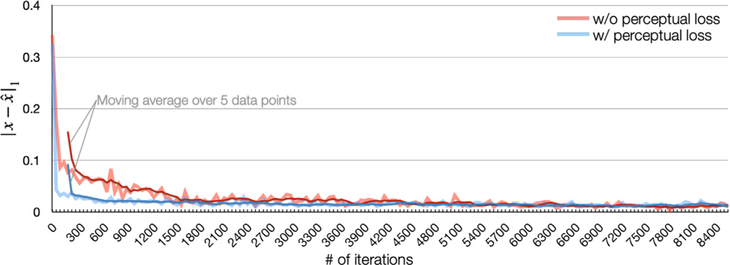
There are some interesting observations in our ablation study. First, the proposed 3D fusion network significantly improves harmonization performance in most cases, as can be observed from the fifth row and the last row in Table 3. Second, the perceptual loss does not have significant benefits to the final harmonization performance (last two rows of Table 3), which is surprising to us. However, the network converges faster with the perceptual loss, as we show in Appendix D.

3.3. Domain adaptation

Fig. 10 provides a visual comparison before and after domain adaptation (DA). The goal is to harmonize images from Site $C$ to Site $D$ using a model trained on Sites $A$ and $D$. We note that the clusters for Sites $A$, $C$, and $D$ are separate in Fig. 8; the example images from Sites $C$ and $D$ shown in Fig. 10 (a) and (e), respectively, illustrate the differences in appearance of ${\text{T}}_1$ images from these sites. We show results from three different harmonization strategies in Fig. 10. In Fig. 10 (b), we show a result from direct harmonization without DA. Like most ML approaches, without any adjustment the harmonization model is unlikely to handle the domain shift between the training and testing. For example, note the appearance of the cerebellar region highlighted by the red arrow. The result on the same image after harmonization using DA is shown in Fig. 10 (c). As described above, DA is achieved by fine tuning on a subset of Site $C$ images without any images from Sites $A$ and $D$. For comparison, we show in Fig. 10 (d) the result obtained on this test image after retraining using data from all three sites. As can be expected, a retraining produces the most satisfactory harmonization result. But when such retraining is not possible, fine tuning using domain adaptivity provides a better result than application of the original network.

Fig. 10.

Results of domain adaptation. The proposed model is trained on Sites $A$ and $D$, and the task is to harmonize images from Site $C$ to Site $D$ during testing. From left to right: (a) the original image from Site $C$; (b) harmonization without domain adaptation; (c) harmonization with domain adaptation; (d) harmonization after a retraining that includes Sites $A$, $C$, and $D$; (e) target image (the same subject imaged at Site $D$). Red arrow indicates a bad harmonization in the cerebellum region without domain adaptation.

To quantitatively evaluate the domain adaptivity, we used the held-out traveling subjects from Sites $C$ and $D$. In each experiment, images from only one of the two sites combined with Site $A$ was included in training. During testing, the model was fine tuned on the unseen site (either Site $C$ or $D$) using the strategy described in Section 2.4. We learned from Fig. 10 that even without fine tuning CALAMITI shows some generalizability capability. Therefore, we applied two strategies to prevent a drastic change in network weights during fine tuning. First, we applied a lower learning rate (1∕5 ^th) in fine tuning than the original training. Second, only a fraction of $E_{\beta }$ and $E_{\theta }$ parameters are updated (see Section 2.4 for more details). Note that Sites $E$ and $F$ were not included in the evaluation because they have similar acquisition parameters and contrasts and the model generalizes well in this case. This is also reflected in Fig. 8, where $\theta$ values of Site $E$ and $F$ are more closely clustered than those of Sites $C$ and $D$. Results in Table 4 show significant improvements ($p<.05$, $N=10$) after DA using a paired Wilcoxon signed rank test, where the null hypothesis is that the difference of SSIM or PSNR between the two methods are of zero median.

Table 4.

Quantitative evaluation of domain adaptation. Images from Site $A$ and one of Sites $C$ and $D$ are included in the training. We report SSIM and PSNR; higher values are better for both.

Training	Testing		Before DA	After DA
$A$,	$C\to$	SSIM	0.8359 ± 0.0253	0.8480 ± 0.0287
$D$	$D$	PSNR	27.76 ± 0.57	29.07 ± 0.71
$A$,	$D\to$	SSIM	0.7893 ± 0.0216	0.7990 ± 0.221
$C$	$C$	PSNR	27.12 ± 0.47	27.51 ± 0.52

3.4. Segmentation consistency

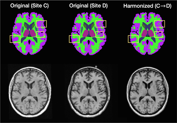
To show that CALAMITI alleviates segmentation inconsistency caused by inter-site contrast variations, we applied SLANT (Huo et al., 2019), a deep learning based whole brain parcellation algorithm, to both the original and harmonized MR images. The original output of SLANT contains 133 labels including the background. For simplicity of reporting, the SLANT labels were merged into background and nine other labels: ventricles, cerebellum GM, cerebrum GM, caudate, thalamus, puta-men, brainstem, cerebellum WM, and cerebrum WM. The images used in this experiment are the traveling subjects from Sites $C/D$ and $E/F$, and therefore we would expect SLANT to produce the same segmentation result for each pair of inter-site scans. From left to right in Fig. 11, we have the Site $C$ acquisition, the Site $D$ acquisition, and the harmonized (from $C$ to $D$) image, with the ${\text{T}}_1-\text{w}$ MR images on the bottom and corresponding SLANT images above. We observe that, although the MR images are from the same subject, the SLANT results are different due to the contrast variation across sites. As highlighted by the yellow boxes, SLANT produces more consistent segmentation results on the harmonized image compared with the original unharmonized image. That is, the right-most segmentation image more closely resembles the center segmentation than the left-most segmentation.

Fig. 11.

A visual comparison of segmentation on a traveling subject. From left to right are Site $C$ acquisition, the Site $D$ acquisition, and the harmonized (from $C$ to $D$) image. The bottom row are the ${\text{T}}_1-\text{w}$ MR images and the top row are the corresponding SLANT (Huo et al., 2019) segmentation. Yellow boxes highlight improved segmentation consistency after harmonization.

To quantitatively evaluate the effects of harmonization on segmentation, we performed an experiment using the two sources of traveling subjects. In each experiment, both Dice coefficient and percentage volume difference (PVD) were calculated. The Dice coefficient between two binary masks is defined as

$$\text{Dice}(𝓐,𝓑)=\frac{2|𝓐\cap 𝓑|}{\left|𝓐\right|+\left|𝓑\right|},$$

where $𝓐$ and $𝓑$ are the binary masks for a given label, and $|\cdot |$ denotes the number of voxels. PVD between two binary labels with 1 mm ³ voxels is defined as

$$\text{PVD}(𝓐,𝓑)=\frac{\left|𝓐\right|-\left|𝓑\right|}{\left|𝓑\right|}\times 100\text{\%}.$$

Note that there is no ground truth labels in this segmentation task, and the goal is to evaluate the segmentation consistency before and after harmonization. For no harmonization (“no har ”), $𝓐$ and $𝓑$ represent the segmentation labels of the original MR images from the source site and the target site, respectively. In comparing different harmonization results, $𝓐$ represents segmentation labels of harmonized images from the source site to the target site, and $𝓑$ represents segmentation labels of self-reconstructed images from the target site. This is to reduce other effects (e.g., noise levels) that are irrelevant to contrast. If harmonization improves segmentation consistency, we could expect an increased Dice coefficient and a PVD that is smaller in magnitude.

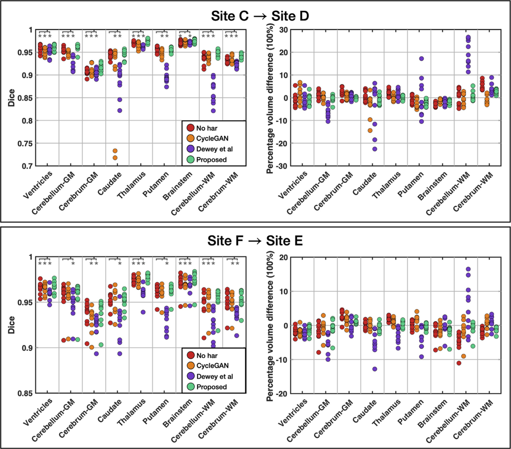
Our first experiment involves harmonization from Site $C$ to Site $D$. As shown in Table 2 and Fig. 6, the two sites have quite different acquisition parameters and contrasts, where Site $C$ has worse GM/WM contrast than Site $D$. As shown in the top row of Fig. 12, an overall trend of increased Dice coefficient and closer-to-zero PVD can be observed after applying the proposed method. Asterisks in the figure indicate statistical significance ($p<.05$, $N=10$) with paired Wilcoxon signed rank tests between the proposed method and the others. The null hypothesis is that the difference between two measurements is drawn from a distribution with zero median. These results show that CALAMITI has significantly higher Dice coefficient than no harmonization in 8 out of 9 labels; it also outperforms the comparison methods in most labels. CALAMITI also shows improvements over no harmonization and other methods in most regions, although no statistical differences are observed. Results for the thalamus and the cerebrum WM are of particular interest because SLANT tends to yields larger volumes than the locally-trained results when no DA is carried out. CALAMITI harmonization yields PVDs that are closer to zero.

Fig. 12.

Strip plot of the Dice coefficient and percentage volume difference before and after harmonization. Wilcoxon signed rank tests are conducted on Dice coefficient between the proposed method and the other methods. Asterisks indicate significance with respect to a $p<.05$ and $N=10$.

Our second experiment considers a harmonization scenario in which the two sites have similar acquisition parameters and contrasts (see Sites $E$ and $F$ in Table 2 and Fig. 6). We make three observations about the resulting Dice and PVD plots, which are shown on the bottom row of Fig. 12. First, without harmonization (“no har ”), all 9 labels have relatively high Dice coefficients and low absolute PVD values compared with the top row of Fig. 12; this is expected due to the similarity in image contrasts in the two sites. Second, using Wilcoxon tests as in the previous experment, we observe that there are 4 out of 9 labels showing significant differences. Since all of these differences favor CALAMITI, we can maintain that for MR images with similar acquisition parameters and contrasts, the proposed method can still boost segmentation consistency. Third, although CALAMITI is built upon Dewey et al.’s method (Dewey et al., 2020), it shows significant improvements over (Dewey et al., 2020) in multiple measurements. We hypothesize that the improvements are due to the globally disentangled latent space, the fusion network, and the IB theory used in our model design.

4. Discussion and future work

4.1. Discussion

In this work, we proposed CALAMITI, a new method for site-level MR harmonization. CALAMITI is a paradigm shift away from CycleGAN based methods and supervised harmonization methods using traveling subjects; it takes advantage of the available intra-site multi-contrast MR images, which are commonly acquired in many MR imaging sessions. We demonstrated CALAMITI by focusing on ${\text{T}}_1-\text{w}$ and ${\text{T}}_2-\text{w}$ images. Our experiments show that CALAMITI improves contrast similarity in multi-site brain MR data. Our 10-site harmonization experiment showcases the broad applicability of our method. In particular, we can achieve translation between different ${\text{T}}_1$-weighted images that are acquired with different field strengths, scanner types, and pulse sequence parameters (see Table 2). We highlight the qualitative demonstrations of harmonization in Fig. 6 and the quantitative evaluations in Table 3, in which we performed an inter-site harmonization using traveling subjects not included in training. Note that CALAMITI only requires a single image to use after training as demonstrated by Section 2.1 and the $\beta$-space interpolation in Fig. 8.

In Table 3, we show that CALAMITI improves the SSIM and PSNR after harmonization. More importantly, we demonstrate in Fig. 12 that the downstream segmentation task has shown improved consistency after harmonization. The mean Dice coefficients of the segmentation labels, before and after harmonization, are always better for CALAMITI over the competing methods, and it is significantly better in 19 of the 27 statistical tests. The fact that the mean percentage volume differences (mean PVDs) are closer to zero indicates that the segmentation is less biased after harmonization.

We also observe that this work answers a long-standing question in the community: In neuroimage analysis, is it good enough to have two similar scanners with similar imaging parameters, or can harmonization improve our analyses? In Table 3, when considering the harmonization between Sites $E$ and $F$, we are addressing this question; see Table 2 and Fig. 6 for the similarity in the scanners, sequences, and image contrasts at Sites $E$ and $F$. We show that a higher SSIM and PSNR can still be achieved in this case, as well as an improved segmentation consistency.

Despite the limitations we discuss in Section 4.2, our approach offers several interesting possibilities in neuroimage analyses. For example, multi-site studies that have previously been explored using segmentation alone (e.g., the ABIDE study (Martino et al., 2014), BLSA study Resnick et al. (2000), Han et al. (2020) could be augmented using voxel-based morphetry after harmonization. We could also take advantage of our $\theta$ space given that it does a very good job in clustering contrast variability caused by scanner and acquisition differences (see Fig. 8). For example, computation of $\theta$ could serve to identify scans that have been acquired with incorrect imaging parameters. We note that $E_{\theta }$ is sensitive enough to capture contrast differences that are hardly noticeable to the human eye (e.g., Sites $E$ and $F$ in Fig. 8). Therefore, even within a single site, harmonization of images could be beneficial for consistency of downstream analyses. It is worth mentioning that there is no site or modality labels used in training our $\theta$-encoder. Therefore, our $\theta$ space is learned in a completely data-driven manner, which we regard as an important feature. Introducing a $\theta$-classifier (or discriminator) to push $\theta$ to capture domain-specific information is redundant and not desired in CALAMITI. From our experiments, Sites $D$ and $E$ have identical acquisition parameters, thus they have overlapping $\theta$ clusters. This was not forced with any additional loss but discovered in a completely data-driven manner. Introducing a $\theta$ classifier to distinguish $\theta$’s of Sites $D$ and $E$ would force an artificial $\theta$ separation, which is undesirable.

The unified network structure of our approach offers several tantalizing possibilities. First, our $\theta$ space is a rich area for research. We have some initial exploration in Fig. 9, in which we demonstrate interpolation in this space. We observe variations in ${\text{T}}_1-\text{w}$ images on the right of Fig. 9, while having a more interesting transition from ${\text{T}}_1-\text{w}$ to ${\text{T}}_2-\text{w}$ on the left. This essentially makes our $\theta$ space and our decoder a powerful image synthesis tool that allows for a more straightforward interpolation in the latent $\theta$ space compared with existing works. Compared with StarGAN Choi et al. (2018), for example, the proposed method offers interpretability and flexibility during image synthesis. Due to the unified CVAE structure, image synthesis can be achieved by simply sampling a target $\theta$ value in the $\theta$ space and combining it with a $\beta$ map to the decoder. In contrast, the method of Jog et al. (2015) requires solving a highly nonlinear imaging equation to generate new contrasts, which is a computationally unstable challenge. The second possibility arising from the unified structure of our approach is that it becomes possible, in principle, to train on an ever-expanding number of sites and contrasts. In this case, the decoder might generalize to handle an arbitrarily large number of scanner types and, in combination with the $\theta$ space interpolation, would yield a universal digital MR scanner that can generate any MR contrast. This capability, in turn, might open the door for task-specific synthesis, where the goal is to generate synthetic images that elucidate a particular feature or structure that facilitates specific downstream tasks. A third potential benefit of our approach is that the IB theory used in its design enables the information encoded by $E_{\theta }$ to be quantified. Measuring such information in a deep network model could be helpful in understanding the model behavior. In CALAMITI, we show the connection between IB theory and the disentangling using a conditional VAE, which is well understood and theoretically attractive. It is worth mentioning that there are alternative formulations to achieve disentangling. For example, one could minimize $I$ ($X$; $X^{\prime }$|$\theta$) to encourage the conditional independence between $X$ and $X^{\prime }$, and extract the common (i.e., contrast) information between $X$ and $X^{\prime }$. Finally, our $\beta$ space is domain-invariant after training, as it captures anatomical information. Atlason et al. (2019) and Chartsias et al. (2019) have shown that domain-invariant representations can help produce improved segmentation results in multiple tasks.

4.2. Limitations

Our work has some limitations. The chief limitation is the inherent assumption that the anatomical information from the intra-site ${\text{T}}_1-\text{w}$ and ${\text{T}}_2-\text{w}$ images is the same. On the surface, when acquiring ${\text{T}}_1-\text{w}$ and ${\text{T}}_2-\text{w}$ images of the same subject, we would expect that they represent the same anatomy. However, the very reason for obtaining multi-contrast images with different pulse sequences is that they reflect different aspects of the anatomy. This issue is particularly apparent when considering patients with WM lesions or brain tumors since these structures appear differently depending on the MR sequences. Additionally, other factors such as resolution, field of view, and artifacts could also contribute to the anatomy differences in the intra-site MR images. Examining how sensitive our training is to these differences in anatomy is an important future research direction. This also brings us to rethink the necessity of the intra-site paired images for our method. We believe training with intra-site paired images is a reasonable requirement for two reasons. First, it is obvious that this requirement is less onerous than acquiring multiple traveling subjects as in most supervised harmonization methods. Second, the intra-site paired images make it possible to train our unsupervised harmonization model in a supervised way, which preserves geometry better over harmonization methods that use cycle consistency. Although cycle consistency is routinely used in most unsupervised IIT approaches, its fundamental assumption is that the image translation function $f(\cdot )$ is bijective. However, for MR imaging, the bijectivity is an arguable assumption since the same MR image could be acquired using different pulse sequences. We also note that there are instances and populations—pediatric cohorts for example —which make it impractical to acquire multiple images using different pulse sequences of a subject in the same session. In such cases, the proposed method cannot be directly applied. Fortunately, there are potential remedies —such as ${\text{T}}_1-\text{w}$ to ${\text{T}}_2-\text{w}$ synthesis —which we have not explored in this paper.

According to our experiments in Section 3.3, domain adaptivity enables our model to provide satisfactory results after fine tuning on a new testing site. However, the fine tuning process is theoretically flawed according to Goodfellow et al. (2020). To properly train a generative adversarial network (GAN), the generator (our $E_{\beta }$) and discriminator (our $D_{\beta }$) must be trained jointly with both positive (Site $A$) and negative (non-Site $A$) training instances. Unfortunately, in our fine tuning process, due to the absence of Site $A$ images, our model is only fed with negative examples, and only $E_{\beta }$ is updated. Although we take actions that restrict both the trainable parameters and the learning rate during fine tuning (see Section 2.4) to improve practical performance, there is still a risk of causing stability issues since $E_{\beta }$ and $D_{\beta }$ are not updated jointly. As for the single-site $D_{\beta }$, we do not regard this as a limitation of this work. Had our $\beta$-discriminator classified whether an input $\beta$ comes from Sites $A$ and $B$ (two sites) or not, then the $\beta$-discriminator is still a one-class discriminator. In which case it also permits domain adaptation but the $\beta$ distributions of Sites $A$ and $B$ could be different.

Our fusion network (see Section 2.5) achieves better slice-to-slice consistency compared with the median filtering approach for combining multi-orientations images (Dewey et al., 2018; 2019). However, our fusion network and the harmonization network are not trained end-to-end due to the GPU memory limit, which implies that our result is not likely to be optimal. We also note that as our decoder, $E_{\beta }$, and $E_{\theta }$ form a generative model, we can use the decoder to generate new contrast MR images by sampling our $\theta$ space. Unfortunately, the failure to train the fusion network end-to-end with the decoder means that we cannot fuse new contrast images created by the decoder. This also explains why the presented interpolations of the $\theta$ space (see Fig. 9) are based on the median filtering approach instead of the proposed fusion network.

There are three areas of concern in our use of the longitudinal scans in the OASIS3 dataset as traveling subjects. First, although the mean Dice coefficient increases in both harmonization scenarios (Sites $C$ to $D$ and Sites $F$ to $E$), there are particular subjects and labels that experience a decrease in their Dice coefficients. This may be due in part to random noise effects, or it may point to other issues such as “corner cases ” for which our framework is somehow detrimental. The same can be observed for some subjects and labels with respect to the PVD criterion. A second concern is the size of the traveling subject cohort used in our quantitative evaluation. Although our experiments include a diverse set of MR data (see Table 2), there are limited numbers of subjects in the quantitative evaluation. To our knowledge, there are very limited public traveling subject data that have been imaged on two scanners within a small window of time. Future studies would benefit from evaluation using a larger cohort from more diverse sites. Finally, our evaluation on downstream processing is exclusively based on SLANT Huo et al. (2019) segmentation results. Although we argue that SLANT is a state-of-the-art whole brain segmentation method that serves to demonstrate the potential for improvement through CALAMITI harmonization, we acknowledge that there are a host of other processing objectives and methods that should be explored in the future.

4.3. Future work

In addition to previously noted potential future work, we point out six additional promising directions for future work. First, to further reduce the requirements on training data and increase the applicability of the proposed method, it is worth exploring the possibility of creating synthetic intra-site paired data. In this case, harmonization from just one MR contrast may become possible. On the other hand, if more than two MR contrasts are available at a given site, it would be interesting to explore the utility of such data in disentanglement and harmonization. Second, a deeper understanding of the theory of domain adaptation is needed since many domain adaptation works He et al. (2020a, 2020b, 2021) suffer from the theoretical dilemma that we discussed in Section 4.2. Despite its importance, domain adaptation of medical image analysis methods remains an open issue in the community. Third, in our quantitative evaluation, CALAMITI achieves satisfactory domain adaptivity between Sites $C$ and $D$. However, we believe the domain adaptivity is not unlimited; there exists a boundary such that the domain adaption would break down when the new testing site has drastically different contrast than the training sites. Given the 10 training sites, we were not able to test the boundary of our network, and we regard this as a direction that should be explored in future work. Fourth, the presented work has focused exclusively on healthy controls. This was done to explore the idea, develop the framework, and demonstrate the utility of the proposed approach. Although many novel medical image analysis methods were introduced in this same way, the suitability of CALAMITI in pathological cases must be evaluated to establish more general utility. Fifth, CALAMITI disentangles anatomical and pulse sequence based contrast information into latent representations $\beta$ and $\theta$, respectively. However, there are other factors that could confound the disentangling process. For example, the signal intensity of MR imaging and the brain morphology both change with age (Salonen et al., 1997). Whether such aging effects should be encoded in $\beta$ or $\theta$ is unclear. Furthermore, we assume that the MR images from all sites are coming from the same anatomical distribution. This assumption, in conjunction with our $D_{\beta }$, provides us with a globally disentangled $\beta$ space. However, when the sites have different age distributions (e.g., pediatric and adult brains), the underlying anatomical information is differently distributed in nature. Although, we did not observe noticeable age effects in our harmonization experiments given that our 10 sites have slightly different age distributions, we believe aging could play a role in harmonization and should be explored in future work. Lastly, in addition to exploring alternative downstream processing objectives, as mentioned above, it is necessary to explore the impact of such tasks on medical research and/or clinical medicine. For example, although we envision CALAMITI as a tool for harmonizing MRI images for multi-site studies, this remains to be done. Whether CALAMITI will permit us to expand such clinical studies to ever increasing number of subjects across sites is an important question that needs to be answered in the future.

5. Conclusion

In this article, we proposed an unsupervised MR harmonization approach, CALAMITI, that harmonizes multi-contrast multi-site MR images without inter-site paired images (i.e., traveling subjects). CALAMITI overcomes common drawbacks of traditional unsupervised harmonization methods while having the merits of multiple existing image-to-image translation approaches. The domain adaptability enables our model to work on a new testing site with a straightforward fine-tuning process. Furthermore, we established CALAMITI using IB theory, and used it to guide our model design, which provides a theoretical basis for the overall approach. Extensive experiments on a 10-site harmonization show that CALAMITI achieves state-of-the-art harmonization performance across sites. Results on the downstream task of whole-brain segmentation shows improved consistency after harmonization, showing potential for its application to large-scale multi-site studies.

Appendix A. Proof of Theorem 1

Proof. To show that optimizing Eq. (5) is equivalent to optimizing the CVAE loss in Eq. (6), we consider the two terms in Eq. (5) separately. Using the definition of mutual information, it is easy to show that

$$I\left(X^{\prime };\theta \right)={\mathbb{E}}_{p\left(x^{\prime }\right)}\left[{𝓓}_{\text{KL}}\left[p\left(\theta \mid x^{\prime }\right)\parallel p(\theta )\right]\right].$$

For $I(X;\theta \mid \tilde{\beta })$, we have

$$\begin{gathered} I(X;\theta \mid \tilde{\beta }) \\ =H(X\mid \tilde{\beta })-H(X\mid \theta ,\tilde{\beta }) \\ =H(X\mid \tilde{\beta })+\sum _x\sum _{\tilde{\beta }}\sum _{\theta }p(x,\theta ,\tilde{\beta })\log p(x\mid \theta ,\tilde{\beta }) \\ =H(X\mid \tilde{\beta })+\sum _x\sum _{x^{\prime }}\sum _{\tilde{\beta }}\sum _{\theta }p\left(x,x^{\prime },\theta ,\tilde{\beta }\right)\log p(x\mid \theta ,\tilde{\beta }) \\ =H(X\mid \tilde{\beta })+\sum _{x^{\prime }}\sum _x\sum _{\tilde{\beta }}\sum _{\theta }p\left(x^{\prime }\right)p\left(x,\tilde{\beta },\theta \mid x^{\prime }\right)\log p(x\mid \theta ,\tilde{\beta }) \\ =H(X\mid \tilde{\beta })+\sum _{x^{\prime }}\sum _x\sum _{\tilde{\beta }}\sum _{\theta }p\left(x^{\prime }\right)p\left(x,\tilde{\beta }\mid x^{\prime }\right)p\left(\theta \mid x^{\prime }\right)\log p(x\mid \theta ,\tilde{\beta }) \\ =H(X\mid \tilde{\beta })+\sum _{x^{\prime }}\sum _x\sum _{\tilde{\beta }}p\left(x,x^{\prime },\tilde{\beta }\right)\sum _{\theta }p\left(\theta \mid x^{\prime }\right)\log p(x\mid \theta ,\tilde{\beta }) \\ =H(X\mid \tilde{\beta })+{\mathbb{E}}_{p\left(x,x^{\prime },\tilde{\beta }\right)}\left[{\mathbb{E}}_{p\left(\theta \mid x^{\prime }\right)}[\log p(x\mid \theta ,\tilde{\beta })]\right]. \end{gathered}$$

In the above derivation, we assume the conditional independence that $p\left(x,\tilde{\beta },\theta \mid x^{\prime }\right)=p\left(x,\tilde{\beta }\mid x^{\prime }\right)p\left(\theta \mid x^{\prime }\right)$. This conditional independence holds because the only common information between $x$ and $x^{\prime }$ is contrast, and therefore given $x^{\prime }$, observing $\theta$ provides no extra information about $x$ or $\tilde{\beta }$, and vice versa.

Combining the two terms, Eq. (5) becomes

$$\begin{gathered} {\theta }^{\ast }=\underset{\theta }{\text{arg}\text{min}}I\left(X^{\prime };\theta \right)-\lambda I(X;\theta \mid \tilde{\beta }) \\ =\underset{\theta }{\text{arg}\text{min}}{\mathbb{E}}_{p\left(x^{\prime }\right)}\left[{𝓓}_{\text{KL}}\left[p\left(\theta \mid x^{\prime }\right)\parallel p(\theta )\right]\right]- \\ \lambda \left[H(X\mid \tilde{\beta })+{\mathbb{E}}_{p\left(x,x^{\prime },\tilde{\beta }\right)}\left[{\mathbb{E}}_{p\left(\theta \mid x^{\prime }\right)}[\log p(x\mid \theta ,\tilde{\beta })]\right]\right] \\ =\underset{\theta }{\text{arg}\text{min}}{\mathbb{E}}_{p\left(x^{\prime }\right)}\left[{𝓓}_{\text{KL}}\left[p\left(\theta \mid x^{\prime }\right)\parallel p(\theta )\right]\right]- \\ \lambda \left[{\mathbb{E}}_{p\left(x,x^{\prime },\tilde{\beta }\right)}\left[{\mathbb{E}}_{p\left(\theta \mid x^{\prime }\right)}[\log p(x\mid \theta ,\tilde{\beta })]\right]\right] \\ =\underset{\theta }{\text{arg}\text{min}}\frac{1}{N}\sum _{i=1}^N{𝓓}_{\text{KL}}\left[p\left(\theta \mid x_i^{\prime }\right)\parallel p(\theta )\right]- \\ \lambda {\mathbb{E}}_{p\left(\theta \mid x_i^{\prime }\right)}\left[\log p\left(x_i\mid \theta ,{\tilde{\beta }}_i\right)\right], \end{gathered}$$

where the outside expectations are approximated by the empirical mean, and $N$ is the number of training instances. □

Fig. 13.

Shown are the original sagittal orientation of ${\text{T}}_1-\text{w}$ MR images from 10 sites and their corresponding harmonized images for Sites $A$, $E$, and $J$.

Appendix B. Qualitative harmonization results of ${\text{T}}_1-\text{w}$ images

Fig. 13 shows the sagittal orientation for a 10-site harmonization experiment.

Appendix C. Qualitative harmonization results of ${\text{T}}_2-\text{w}$ images from a sagittal view

Fig. 14 shows the harmonization results of ${\text{T}}_2$ images.

Fig. 14.

Shown are the original ${\text{T}}_2-\text{w}$ MR images from 10 sites and their corresponding harmonized images for Sites $A$.

Fig. 15.

The $l_1$ reconstruction error with respect to the number of training iterations.

Appendix D. An ablation study on the perceptual loss

We conducted an ablation study to show the effects of the perceptual loss. In the experiment, we kept all the hyperparameters the same, the only difference is the presence of the perceptual loss. According to our study, we found no significant difference in SSIM and PSNR of the harmonized images (see Table 3), but adding a perceptual loss helps the network converge faster, as shown in Fig. 15.

References

- American College of Radiology, 2018. Phantom test guidance for use of the large MRI phantom for the ACR MRI accreditation program. Released: 4/17/18. https://www.acraccreditation.org/-/media/ACRAccreditation/Documents/MRI/LargePhantomGuidance.pdf. [Google Scholar]
- Atlason HE, Love A, Sigurdsson S, Gudnason V, Ellingsen LM, 2019. Unsupervised brain lesion segmentation from MRI using a convolutional autoencoder. In: Medical Imaging 2019: Image Processing, Vol. 10949. International Society for Optics and Photonics, p. 109491H. [Google Scholar]
- Brown RW, et al. , 2014. Magnetic Resonance Imaging: Physical Principles and Sequence Design (Second Edition). Wiley. [Google Scholar]
- Chartsias A, Joyce T, Papanastasiou G, Semple S, Williams M, Newby DE, Dharmakumar R, Tsaftaris SA, 2019. Disentangled representation learning in cardiac image analysis. Med. Image Anal 58, 101535. [DOI] [PMC free article] [PubMed] [Google Scholar]
- Choi Y, Choi M, Kim M, Ha J-W, Kim S, Choo J, 2018. Stargan: unified generative adversarial networks for multi-domain image-to-image translation. In: Proceedings of the IEEE Conference on Computer Vision and Pattern Recognition, pp. 8789–8797. [Google Scholar]
- Cohen JP, Luck M, Honari S, 2018. Distribution matching losses can hallucinate features in medical image translation. In: Proceedings of the International Conference on Medical Image Computing and Computer-assisted Intervention. Springer, pp. 529–536. [Google Scholar]
- Dai B, Zhu C, Guo B, Wipf D, 2018. Compressing neural networks using the variational information bottleneck. In: Proceedings of the International Conference on Machine Learning. PMLR, pp. 1135–1144. [Google Scholar]
- Dewey BE, Zhao C, Carass A, Oh J, Calabresi PA, van Zijl PCM, Prince JL, 2018. Deep harmonization of inconsistent MR data for consistent volume segmentation. In: Proceedings of the Workshop on Simulation and Synthesis in Medical Imaging (SASHIMI) Held in Conjunction with the 21st International Conference on Medical Image Computing and Computer Assisted Intervention (MICCAI 2018). Springer Berlin Heidelberg, pp. 22–30. [Google Scholar]
- Dewey BE, Zhao C, Reinhold JC, Carass A, Fitzgerald KC, Sotirchos ES, Saidha S, Oh J, Pham DL, Calabresi PA, 2019. DeepHarmony: a deep learning approach to contrast harmonization across scanner changes. Mag. Reson. Imaging 64, 160–170. [DOI] [PMC free article] [PubMed] [Google Scholar]
- Dewey BE, Zuo L, Carass A, He Y, Liu Y, Mowry EM, Newsome S, Oh J, Calabresi PA, Prince JL, 2020. A disentangled latent space for cross-site MRI harmonization. In: Proceedings of the 23rd International Conference on Medical Image Computing and Computer Assisted Intervention (MICCAI 2020). Springer, pp. 720–729. [Google Scholar]
- Fortin J-P, Parker D, Tunç B, Watanabe T, Elliott MA, Ruparel K, Roalf DR, Satterthwaite TD, Gur RC, Gur RE, Schultz RT, Verma R, Shinohara RT, 2017. Harmonization of multi-site diffusion tensor imaging data. Neuroimage 161, 149–170. [DOI] [PMC free article] [PubMed] [Google Scholar]
- Garcia-Dias R, Scarpazza C, Baecker L, Vieira S, Pinaya WH, Corvin A, Redolfi A, Nelson B, Crespo-Facorro B, McDonald C, et al. , 2020. Neuroharmony: a new tool for harmonizing volumetric MRI data from unseen scanners. Neuroimage 220. [DOI] [PMC free article] [PubMed] [Google Scholar]
- Goodfellow I, Pouget-Abadie J, Mirza M, Xu B, Warde-Farley D, Ozair S, Courville A, Bengio Y, 2020. Generative adversarial networks. Commun. ACM 63 (11), 139–144. [Google Scholar]
- Han S, Carass A, He Y, Prince JL, 2020. Automatic cerebellum anatomical parcellation using U-Net with locally constrained optimization. Neuroimage 218, 116819. [DOI] [PMC free article] [PubMed] [Google Scholar]
- He Y, Carass A, Liu Y, Saidha S, Calabresi PA, Prince JL, 2020a. Adversarial domain adaptation for multi-device retinal OCT segmentation. In: Medical Imaging 2020: Image Processing, Vol. 11313. International Society for Optics and Photonics, p. 1131309. [Google Scholar]
- He Y, Carass A, Zuo L, Dewey BE, Prince JL, 2020b. Self domain adapted network. In: Proceedings of the 23rd International Conference on Medical Image Computing and Computer Assisted Intervention (MICCAI 2020). Springer, pp. 437–446. [Google Scholar]
- He Y, Carass A, Zuo L, Dewey BE, Prince JL, 2021. Autoencoder based self-super-vised test-time adaptation for medical image analysis. Med. Image Anal 102136. [DOI] [PMC free article] [PubMed] [Google Scholar]
- Huang X, Liu MY, Belongie S, Kautz J, 2018. Multimodal unsupervised image-to-image translation. In: Proceedings of the European Conference on Computer Vision, pp. 172–189. [Google Scholar]
- Huo Y, Xu Z, Xiong Y, Aboud K, Parvathaneni P, Bao S, Bermudez C, Resnick SM, Cutting LE, Landman BA, 2019. 3D whole brain segmentation using spatially localized atlas network tiles. Neuroimage 194, 105–119. [DOI] [PMC free article] [PubMed] [Google Scholar]
- Jog A, Carass A, Roy S, Pham DL, Prince JL, 2015. Mr image synthesis by contrast learning on neighborhood ensembles. Med. Image Anal 24 (1), 63–76. [DOI] [PMC free article] [PubMed] [Google Scholar]
- Johnson J, Alahi A, Fei-Fei L, 2016. Perceptual losses for real-time style transfer and super-resolution. In: Proceedings of the European Conference on Computer Vision. Springer, pp. 694–711. [Google Scholar]
- Kamnitsas K, Baumgartner C, Ledig C, Newcombe V, Simpson J, Kane A, Menon D, Nori A, Criminisi A, Rueckert D, 2017. Unsupervised domain adaptation in brain lesion segmentation with adversarial networks. In: Proceedings of the International Conference on Information Processing in Medical Imaging. Springer, pp. 597–609. [Google Scholar]
- Kingma DP, Welling M, 2013. Auto-encoding variational Bayes. arXiv preprint arXiv:1312.6114. [Google Scholar]
- LaMontagne PJ, Benzinger TL, Morris JC, Keefe S, Hornbeck R, Xiong C, Grant E, Hassenstab J, Moulder K, Vlassenko A, et al. , 2019. Oasis-3: longitudinal neuroimaging, clinical, and cognitive dataset for normal aging and alzheimer disease. MedRxiv. [Google Scholar]
- Lindvall T, 2002. Lectures on the Coupling Method. Courier Corporation. [Google Scholar]
- Liu AH, Liu YC, Yeh YY, Wang YCF, 2018. A unified feature disentangler for multi-domain image translation and manipulation. In: Proceedings of the Advances in Neural Information Processing Systems, pp. 2590–2599. [Google Scholar]
- Liu M-Y, Breuel T, Kautz J, 2017. Unsupervised image-to-image translation networks. In: Proceedings of the Advances in Neural Information Processing Systems, pp. 700–708. [Google Scholar]
- Liu X, Xing F, El Fakhri G, Woo J, 2021. A unified conditional disentanglement framework for multimodal brain mr image translation. In: Proceedings of the IEEE 18th International Symposium on Biomedical Imaging (ISBI). IEEE, pp. 10–14. [DOI] [PMC free article] [PubMed] [Google Scholar]
- Liu Y, Zuo L, Carass A, He Y, Filippatou A, Solomonand SD, Saidha S, Calabresi PA, Prince JL, 2020. Variational intensity cross channel encoder for unsupervised vessel segmentation on OCT angiography. In: Medical Imaging 2020: Image Processing, Vol. 11313. International Society for Optics and Photonics, p. 113130Y. [Google Scholar]
- Martino AD, Yan C-G, Li Q, Denio E, Castellanos FX, Alaerts K, Anderson JS, Assaf M, Bookheimer SY, Dapretto M, Deen B, Delmonte S, Dinstein I, Ertl-Wagner B, Fair DA, Gallagher L, Kennedy DP, Keown CL, Keysers C, Lainhart JE, Lord C, Luna B, Menon V, Minshew NJ, Monk CS, Mueller S, Müller R-A, Nebel MB, Nigg JT, O’Hearn K, Pelphrey KA, Peltier SJ, Rudie JD, Sunaert S, Thioux M, Tyszka JM, Uddin LQ, Verhoeven JS, Wenderoth N, Wiggins JL, Mostofsky SH, Milham MP, 2014. The autism brain imaging data exchange: towards a large-scale evaluation of the intrinsic brain architecture in autism. Mol. Psychiatry 19, 659–667. [DOI] [PMC free article] [PubMed] [Google Scholar]
- Moyer D, Ver Steeg G, Tax CM, Thompson PM, 2020. Scanner invariant representations for diffusion MRI harmonization. Magn. Reson. Med 84 (4), 2174–2189. [DOI] [PMC free article] [PubMed] [Google Scholar]
- Ouyang J, Adeli E, Pohl KM, Zhao Q, Zaharchuk G, 2021. Representation disentanglement for multi-modal MR analysis. In: Proceedings of the 27th Information Processing in Medical Imaging (IPMI 2021). Springer Berlin Heidelberg, p. InPress. [DOI] [PMC free article] [PubMed] [Google Scholar]
- Pomponio R, Erus G, Habes M, Doshi J, Srinivasan D, Mamourian E, Bashyam V, Nasrallah IM, Satterthwaite TD, Fan Y, et al. , 2020. Harmonization of large MRI datasets for the analysis of brain imaging patterns throughout the lifespan. Neuroimage 208, 116450. [DOI] [PMC free article] [PubMed] [Google Scholar]
- Reinhold JC, Dewey BE, Carass A, Prince JL, 2019. Evaluating the impact of intensity normalization on MR image synthesis. In: Medical Imaging 2019: Image Processing, Vol. 10949. International Society for Optics and Photonics, p. 109493H. [DOI] [PMC free article] [PubMed] [Google Scholar]
- Remedios SW, amd C. Bermudez SR, Patel MB, Butman JA, Landman BA, Pham DL, 2020. Distributed deep learning across multisite datasets for generalized CT hemorrhage segmentation. Med. Phys 47 (1), 89–98. [DOI] [PMC free article] [PubMed] [Google Scholar]
- Resnick SM, Goldszal AF, Davatzikos C, Golski S, Kraut MA, Metter EJ, Bryan RN, Zonderman AB, 2000. One-year age changes in MRI brain volumes in older adults. Cereb. Cortex 10 (5), 464–472. [DOI] [PubMed] [Google Scholar]
- Ronneberger O, Fischer P, Brox T, 2015. U-net: Convolutional networks for biomedical image segmentation. In: Proceedings of the International Conference on Medical Image Computing and Computer-Assisted Intervention. Springer, pp. 234–241. [Google Scholar]
- Roy S, Carass A, Prince JL, 2013. Magnetic resonance image example based contrast synthesis. IEEE Trans. Med. Imag 32 (12), 2348–2363. [DOI] [PMC free article] [PubMed] [Google Scholar]
- Saito K, Watanabe K, Ushiku Y, Harada T, 2018. Maximum classifier discrepancy for unsupervised domain adaptation. In: Proceedings of the IEEE Conference on Computer Vision and Pattern Recognition, pp. 3723–3732. [Google Scholar]
- Salonen O, Autti T, Raininko R, Ylikoski A, Erkinjuntti T, 1997. MRI of the brain in neurologically healthy middle-aged and elderly individuals. Neuroradiology 39 (8), 537–545. [DOI] [PubMed] [Google Scholar]
- Sohn K, Lee H, Yan X, 2015. Learning structured output representation using deep conditional generative models. Adv. Neural Inf. Process. Syst 28, 3483–3491. [Google Scholar]
- Thambisetty M, Wan J, Carass A, An Y, Prince JL, Resnick SM, 2010. Longitudinal changes in cortical thickness associated with normal aging. Neuroimage 52 (4), 1215–1223. [DOI] [PMC free article] [PubMed] [Google Scholar]
- Tishby N, Pereira FC, Bialek W, 1999. The information bottleneck method. In: Proceedings of the 37th Annual Allerton Conference on Communication, Control, and Computing, pp. 368–377. [Google Scholar]
- Tustison NJ, Avants BB, Cook PA, Zheng Y, Egan A, Yushkevich PA, Gee JC, 2010. N4ITK: improved N3 bias correction. IEEE Trans. Med. Imaging 29 (6), 1310–1320. [DOI] [PMC free article] [PubMed] [Google Scholar]
- Varsavsky T, Orbes-Arteaga M, Sudre CH, Graham MS, Nachev P, Cardoso MJ, 2020. Test-time unsupervised domain adaptation. In: Proceedings of the International Conference on Medical Image Computing and Computer-Assisted Intervention. Springer, pp. 428–436. [Google Scholar]
- Wang Z, Bovik AC, Sheikh HR, Simoncelli EP, 2004. Image quality assessment: from error visibility to structural similarity. IEEE Trans. Image Process 13 (4), 600–612. [DOI] [PubMed] [Google Scholar]
- Xia W, Yang Y, Xue JH, 2020. Unsupervised multi-domain multimodal image-to-image translation with explicit domain-constrained disentanglement. Neural Netw. 131, 50–63. [DOI] [PubMed] [Google Scholar]
- Zhao C, Dewey BE, Pham DL, Calabresi PA, Reich DS, Prince JL, 2020. SMORE: a self-supervised anti-aliasing and super-resolution algorithm for MRI using deep learning. IEEE Trans Med Imaging 40 (3), 805–817. doi: 10.1109/TMI.2020.3037187. [DOI] [PMC free article] [PubMed] [Google Scholar]
- Zhu AH, Moyer DC, Nir TM, Thompson PM, Jahanshad N, 2019. Challenges and opportunities in dMRI data harmonization. In: Proceedings of the International Conference on Medical Image Computing and Computer-Assisted Intervention. Springer, pp. 157–172. [Google Scholar]
- Zhu J-Y, Park T, Isola P, Efros AA, 2017. Unpaired image-to-image translation using cycle-consistent adversarial networks. In: Proceedings of the IEEE International Conference on Computer Vision, pp. 2223–2232. [Google Scholar]
- Zuo L, Dewey BE, Carass A, He Y, Shao M, Reinhold JC, Prince JL, 2020. Synthesizing realistic brain MR images with noise control. In: Proceedings of the Workshop on Simulation and Synthesis in Medical Imaging (SASHIMI) held in conjunction with the 23rd International Conference on Medical Image Computing and Computer Assisted Intervention (MICCAI 2020), pp. 21–31. [Google Scholar]
- Zuo L, Dewey BE, Carass A, Liu Y, He Y, Calabresi PA, Prince JL, 2021. Information-based disentangled representation learning for unsupervised MR harmonization. In: Proceedings of the International Conference on Information Processing in Medical Imaging. Springer, pp. 346–359. [Google Scholar]
Associated Data
This section collects any data citations, data availability statements, or supplementary materials included in this article.