Abstract
Sepsis is one of the most challenging health conditions worldwide, with relatively high incidence and mortality rates. It is shown that preventing sepsis is the key to avoid potentially irreversible organ dysfunction. However, data-driven early identification of sepsis is challenging as sepsis shares signs and symptoms with other health conditions. This paper adopts a temporal pattern mining approach to identify frequent temporal and evolving patterns of physiological and biological biomarkers in sepsis patients. We show that using these frequent patterns as features for classifying sepsis and non-sepsis patients can improve the prediction accuracy and performance up to 7%. Most of the temporal modeling approaches adopted in the sepsis literature are based on deep learning methods. Although these approaches produce high accuracy, they generally have limited model explainability and interpretability. Using the adopted methods in this study, we could identify the most important features contributing to the patients’ sepsis incidence, such as fluctuations in platelet, lactate, and creatinine, or evolution of patterns including renal and metabolic organ systems, and consequently, enhance the findings’ clinical interpretability.
Keywords: Sepsis prediction, Temporal network mining, Temporal patterns, Evolving patterns
1. Introduction
Sepsis, defined as “life-threatening organ dysfunction caused by a dysregulated host response to infection” [1], is one of the leading causes of health loss and death worldwide. The numbers of incidence of sepsis and sepsis-related deaths reported worldwide in 2017 have been 48.9 million and 11.0 million, respectively [2]. Septicemia, the triggering cause of sepsis, is ranked among the top four most costly health complications, incurring more than $20 billion to only the USA (5.2% of total USA hospital costs) [3].
A study composed of patients from 6 hospitals in the US shows that although sepsis has been the leading cause of death, it is unlikely to prevent these deaths since most sepsis cases resulting in death are associated with underlying severe chronic conditions. Therefore, they cannot be easily treated by providing better hospital-based care. It is suggested that prevention and care of underlying conditions would be a potential solution to reduce the number of sepsis-associated deaths [4]. Therefore, appropriate therapeutic management of to-be sepsis patients as early as possible might stop further deterioration and irreversible organ dysfunction.
There have been numerous studies focusing on the detection of sepsis progression at early stages. These studies adopt different approaches for predicting sepsis incidents or different stages of sepsis, such as septic shock characterized by more severe conditions of organ systems. The data of different vital signs, laboratory tests, patients’ medical histories, and patients’ demographic information are collected in these studies. Then, various analytical methods, such as traditional machine learning algorithms or more advanced deep learning approaches, are applied to the pre-processed data sets. The objective is to either predict some primary outcomes, such as the onset of sepsis or different stages of sepsis and patients’ outcomes [5, 6, 7, 8], or identify the potentially critical clinical indicators and biomarkers for early prediction of these primary outcomes [9, 10, 11, 12].
One common approach for identification or early detection of sepsis is using different sepsis scoring systems, such as SOFA (Sepsis-related Organ Failure Assessment) [13], PIRO (predisposition, insult, response, organ dysfunction) [14], and SIRS (Systemic Inflammatory Response Syndrome) [15]. However, it is shown that machine learning approaches, in general, out-perform sepsis scoring systems [16].
Furthermore, it is shown that considering the temporal dynamics of different biomarkers and vital signs may improve the performance of predictive models [17, 18]. However, most of the proposed approaches for incorporating the temporal aspects of the data components into the models are using different deep learning architectures, such as temporal convolutional, long short-term memory (LSTM), and recurrent neural networks (RNNs) [19, 20, 21, 22]. Although these approaches might some of the traditional machine learning algorithms outperform, they suffer from limited explainability and interpretability of models and findings [23, 24]. In some applications, the performance of these approaches might outweigh the explainability and interpretability. However, these concepts remain crucial for the proposed approaches’ applicability and adoption in clinical settings [25, 26].
On the other hand, it is shown that the consideration and identification of frequent co-failures of physiological and biological biomarkers, instead of considering these variables individually and independently, can improve the performance of prediction models [27, 28]. Identifying patterns of physiological and biological biomarkers observed more frequently in to-be sepsis patients than nonsepsis sepsis patients can result in a more accurate prediction of sepsis incidence. As these physiological and biological biomarkers are measured frequently in patients, observation of these common patterns can inform the explainability of prediction. One of the most common approaches for modeling simultaneous events in various disciplines is using network representations [29]. The problem of identification of frequent patterns in network analysis and mining literature is called frequent subgraph mining. The typical approach for mining frequent subgraphs in data sets of temporal networks is representing the network as a sequence of equal-width time intervals of static networks. In this representation, each network in the sequence is a static network composed of simultaneous events in the corresponding interval [30]. This type of temporal network transformation to a sequence of static networks might either sacrifice some temporal aspects or impose a computational cost to the mining problem. Here, we consider patterns as the temporal changes observed in the physiological and biological biomarkers and their measurements in subpopulations of patients. Consequently, we consider frequent patterns as changes in different physiological and biological biomarkers and their combinations observed more frequently in patients. Based on these definitions, this study aims to answer the following questions.
Using a data set composed of patients with and without sepsis, how can we mine the frequent patterns in these patients while maintaining information regarding the temporal aspects of their physiological and biological biomarkers’ trajectories represented as networks? Are these patterns frequent and significant enough to inform the sepsis onset prediction? How can the frequent patterns detected inform the clinical interpretability of findings?
To answer these questions, we develop a series of novel algorithms for identifying frequent temporal and evolving patterns. We show that these patterns can improve the performance of sepsis incidence prediction. This paper is organized as follows. First, the data set of this study is described. Then, the criteria used to identify sepsis patients are explained, and the adopted approach for modeling dynamics of physiological and biological biomarkers is discussed. Then, the algorithms adopted for mining frequent patterns and their evolution are explained in detail. Next, the results obtained by applying the proposed algorithms to the data set are provided and discussed. The paper concludes with the limitations of the current study and potential future research direction.
2. Study Population
The data set of this study is composed of retrospectively collected EHR data from two hospitals of a single tertiary care health care system (in total, 1,100 in-hospital beds). The data collection is performed from patients admitted to these hospitals between July 2013 and December 2015. The inclusion criteria consist of patient age ≥18 at arrival, and visit types of inpatient, Emergency Department only, or observational visits.
Subpopulations Definition:
We consider two subpopulations of patients in this study; sepsis and non-sepsis. Based on the definition provided by the established Sepsis-3 guidelines [1] and input from subject matter experts, we considered sepsis as infected patients who have experienced at least one organ dysfunction from 24 hours before the first anti-infective administration to the last administration. We also considered vasopressor administration as a sign of organ dysfunction. Patients are considered infected if they have received at least four days of anti-infective or a positive viral polymerase chain reaction test for influenza. Considering death as in-hospital death or discharge to hospice care, the patients who died while they were under anti-infective administration considered a sepsis patient too [31]. The list of physiological and biological biomarkers representing different organ dysfunction are provided in Table 1. The criteria considered for physiological and biological biomarkers’ failures are provided in Supplementary materials-Table 1.
Table 1:
Organ systems and their associated physiological and biological biomarkers.
| Organ Dysfunction | Response |
|---|---|
|
| |
| Cardiovascular | Systolic blood pressure (SBP) |
| * - Systolic BP | |
| Mean arterial pressure (MAP) | |
|
| |
| Renal | Creatinine |
| (Creatinine - **)/() | |
| Blood Urea Nitrogen (BUN) | |
|
| |
| Hematopoietic | WBC |
| Platelet | |
|
| |
| Metabolic | Lactate |
|
| |
| Gastrointestinal | Bilirubin |
|
| |
| Respiratory | Fraction of inspired oxygen () |
| Pulse oximetry () | |
| / | |
| Oxygen () Source | |
|
| |
| Central Nervous | Glasgow Comma Score |
| Glasgow Best Verbal Response | |
Maximum systolic blood pressure for each observation within 8-hour windows.
Initial creatinine value observed in each visit.
As one of the ultimate goals is to compare and evaluate the power of different types and sets of features and their temporal dynamics for sepsis onset prediction, we create four data sets. These data sets are different based on the amount of information provided for sepsis onset prediction. We consider a window before sepsis onset and try to predict whether, based on the states as defined by the corresponding responses (Table 1), and their temporal patterns and evolution, we can differentiate sepsis patients from non-sepsis patients. We consider this window to be 3, 6, 12, and 24 hours and create one data set corresponding to each window (, and , respectively). This window is shown as the “gap” interval in Figure 1. Also, we only include patients in each data set who have at least 24 hours of hospitalization records before the window. By increasing the window, the number of patients meeting this constraint decreases. For non-sepsis patients, we do not have this limitation. However, we randomly select an equal sample size of non-sepsis patients to create a balanced data set. The characteristics of sepsis and non-sepsis patients in the data sets with different gap intervals are provided in Table 2.
Figure 1:
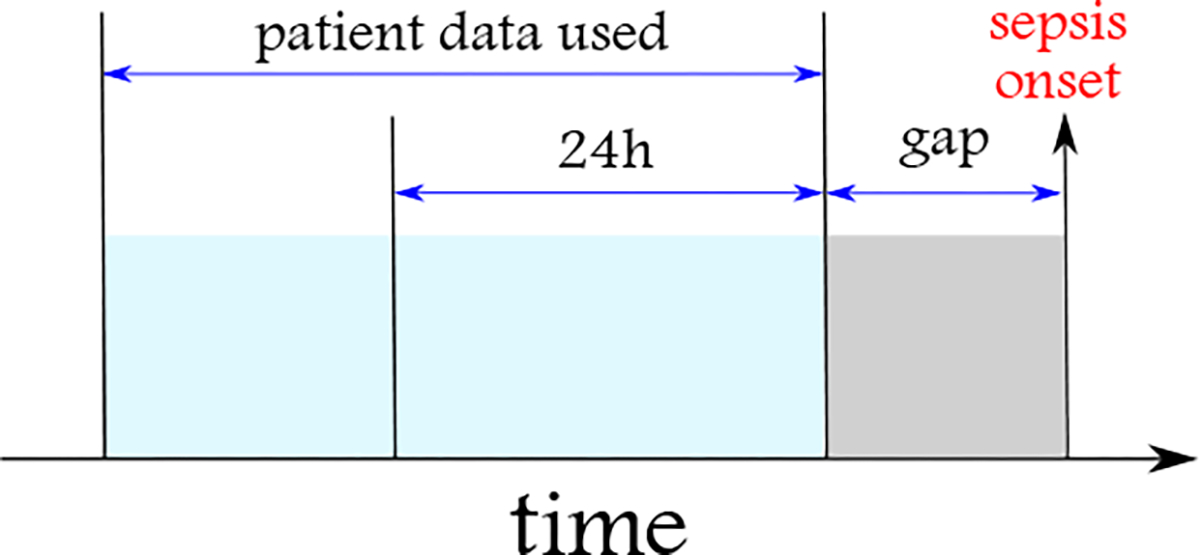
The EHR data used from sepsis patients are composed of responses’ states collected from the beginning of the hospitalization up to a gap (considered as the prediction window into the future) before the onset of sepsis. The prediction windows considered are 3, 6, 12, and 24 hours. The patients should be monitored for at least 24 hours before the gap’s starting time to be included in the study.
Table 2:
A summary of patients characteristics in each subpopulation in four data sets. For sepsis patients in each data set, the data over the course of patients’ hospitalization to h hours prior to the onset of sepsis is considered, i.e., the data collected over the gap period is excluded (for h = 3, 6, 12, and 24 hours).
| 3 hours | 6 hours | 12 hours | 24 hours | |||||
|---|---|---|---|---|---|---|---|---|
| Non-sepsis | Sepsis | Non-sepsis | Sepsis | Non-sepsis | Sepsis | Non-sepsis | Sepsis | |
|
| ||||||||
| Visit count | 3,785 | 3,785 | 3,601 | 3,601 | 3,263 | 3,263 | 2,724 | 2,724 |
| Gender | ||||||||
| Female | 2,412 | 2,023 | 2,312 | 1,919 | 2,029 | 1,739 | 1,662 | 1,422 |
| Male | 1,373 | 1,762 | 1,289 | 1,682 | 1,234 | 1,524 | 1,062 | 1,302 |
| Age in years (mean±SD) | 56±20 | 60-18 | 56±20 | 60±18 | 56±20 | 60±18 | 56±20 | 61±18 |
| Number of comorbidities (n) distribution | ||||||||
| n < 5 | 54.3% | 35.0% | 53.6% | 34.7% | 53.3% | 34.5% | 52.4% | 33.2% |
| 5 ≤ n < 10 | 27.2% | 48.6% | 28.0% | 48.6% | 27.6% | 48.8% | 29.0% | 50.3% |
| n ≥ 10 | 6.4% | 13.5% | 7.0% | 13.6% | 6.2% | 13.7% | 6.8% | 13.9% |
| unknown | 12.1% | 2.9% | 11.4% | 3.1% | 12.9% | 3.0% | 11.8% | 2.6% |
3. Methods
In this study, we use two different approaches to predict the onset of sepsis. The data used for these methods are sepsis and non-sepsis patients’ EHR data. We would like to examine whether we can accurately classify patients into one of the two groups. Therefore, we consider a window before the sepsis incidence onset in sepsis patients. Then, we remove sepsis patients’ data in this window. Also, to accomplish the study’s objectives, we implement different classification algorithms with varying sets of features. More specifically, we use traditional algorithms as baseline methods. Also, we use frequent pattern mining in temporal networks and frequent evolving pattern mining in temporal networks as alternative approaches. The methods are compared based on their performance and other considerations in line with the paper’s objectives. We use different pre-processing and feature engineering steps to implement these methods. In the following, feature engineering is described in detail. Then, the adopted methods are described in further detail.
3.1. Preprocessing & Feature Engineering
The primary features used in this study are 16 physiological and biological biomarkers contributing to organ dysfunctions (Table 1). We also consider the three commonly used sepsis biomarkers; procalcitonin (PRC), C-reactive protein (CRP), and erythrocyte sedimentation rate (ESR). We refer to these 19 features as responses hereafter. Furthermore, age, gender, and past medical history of patients are included as other feature sets.
Considering that vital signs and laboratory tests are generally measured at irregular intervals, using the subject’s matter opinion, we carried forward vital sign measurements for eight hours and lab results for 24 hours if there were no more up-to-date measurements reported in these intervals. Furthermore, some of the variables are derived from a combination of other variables, such as mean arterial pressure () calculated as follows:
| (1) |
where and represent the diastolic and systolic blood pressures, respectively.
This paper aims to identify the most frequent temporal patterns and their evolution in sepsis patients. To compare the usefulness of these patterns, we evaluate their importance in predicting sepsis onset in comparison with the typical approaches adopted in the literature, that is, using different sets of physiological and biological biomarkers as individual features. To accomplish this comparison, we apply multiple traditional machine learning algorithms to the set of individual features. Because the vital signs and lab results change throughout hospitalization, we create various statistics to represent the measures of central tendency (mean and median ) and dispersion (standard deviation and range ) of these features. Therefore, for each of the variables shown in Table 1 and the three biomarkers, we compute these statistics and use them as features to predict the sepsis onset and classify the sepsis patients.
To take the irregularity of inter-measurements into account, we computed the adjusted versions of , , and . In other words, instead of simply computing these statistics, we consider for how long each measurement has been valid. Then, based on these durations at the minute level, we compute , , and . Figure 2 shows how the temporal duration of measurements are included in calculation of , , and . For the range , we do not need to adopt this approach as it does not depend on the time over which the measurement is valid.
Figure 2:
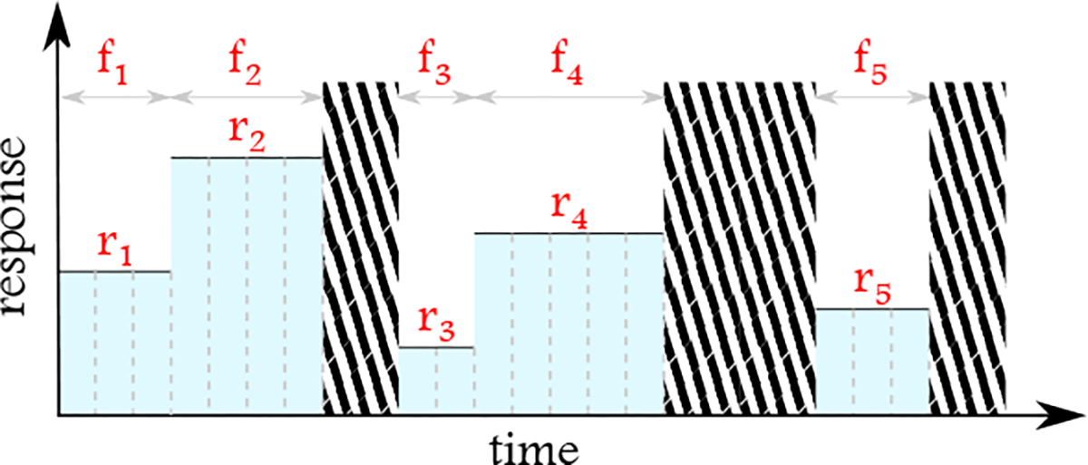
For the computation of mean, median, and standard deviation, in addition to absolute values, the frequency of the corresponding values at the minute level is taken into account. For example, the adjusted mean for the response in this figure would be . The areas with stripes are duration without any values recorded for the response.
3.2. Temporal Networks Construction
For the temporal pattern mining, we create a continuous-time temporal network for each patient. Each network is composed of nodes, representing the responses shown in Table 1 and the three biomarkers and edges, representing the simultaneous measurements of these responses. We consider the networks attributed, and we label each vertex attribute as a vector using the same (adjusted) statistics, . However, contrary to the previous case of individual variables, the labels are separately computed for each interaction window, instead of the entire course of data collection. Note that if during one node’s interaction with another node where the responses are concurrently recorded, the measurements for the same node remain continuously the same, the last two elements in would be zero. Also, note that two nodes might interact at two different intervals with different values of .
Figure 3 shows how continuous-time temporal networks are created for each patient. In Figure 3.a, given a set of responses measured for a patient over time, we identify the overlapping intervals among these responses. The responses are the nodes of the network. The edges represent the window over which each pair of intervals is measured. Figure 3.b provides two representations of the temporal network associated with Figure 3.a. These two representations, edge-based and vertex-based, illustrate the same temporal network. Each row represents one edge and the corresponding window over which the interaction is active in the former. Each row is associated with one response (vertex) in the latter, and interactions are shown with oblique lines spanning over the interaction window. For each patient’s visit in the study population, we create one continuous-time temporal network as explained and record these networks in a network data set, . These networks are used to identify the frequent temporal patterns as described in the following subsection.
Figure 3:
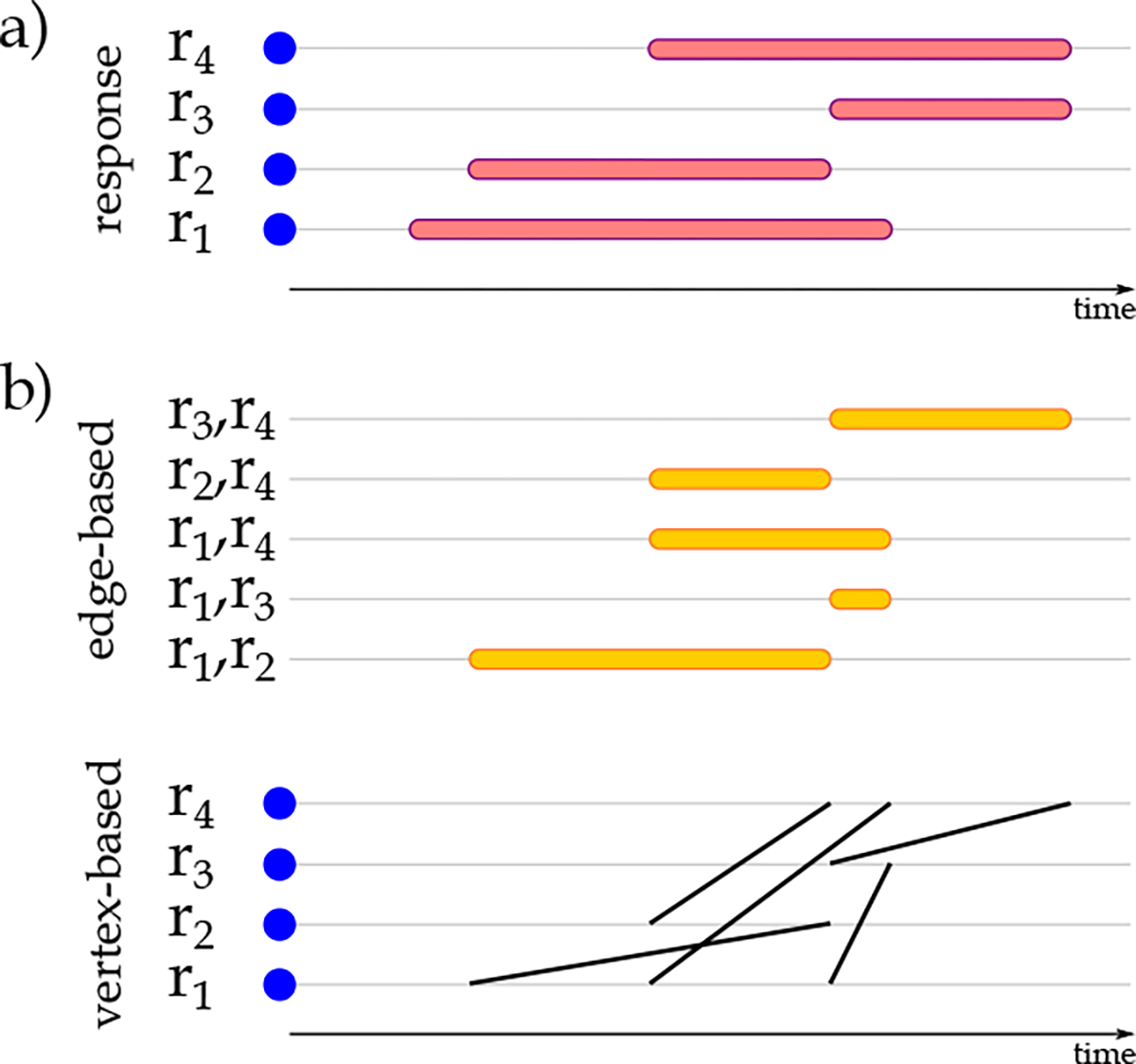
Visualization of physiological and biological biomarkers a) temporal representation of individual physiological and biological biomarkers and b) the edge-based and vertex-based representation of biomarkers’ temporal relationships.
3.3. Frequent Temporal Patterns
Identification of frequent patterns in network data sets has a rich literature in static networks that has attracted increasing attention recently in data sets of temporal networks [30, 32]. The typical approach in the proposed algorithms in the literature is transforming the temporal networks into a set of static networks. This representation might over-represent the interaction times or increase computation time. In this paper, we use the tempowork algorithm proposed for the identification of frequent temporal patterns in a temporal network data set [33]. The implementation of this algorithm is publicly available in the PyPI repository. Once we have the temporal networks data set , we apply the frequent pattern mining algorithms to identify the frequent pattern in .
In [33], each temporal network is converted to a novel graph representation, constrained interval graph , that provides a lossless representation of the associated temporal network. The created for a temporal network are directed networks composed of:
Nodes, , representing the edges in .
Edges, representing overlapping edges in sharing one node.
Each node in is labeled with the nodes’ labels, edge’s label, and the duration of the corresponding edge in . Each edge in is attributed with the delay magnitude between the starting points of the two overlapping edges. Figure 4 visualizes a temporal network at the top and the corresponding at the bottom.
Figure 4:
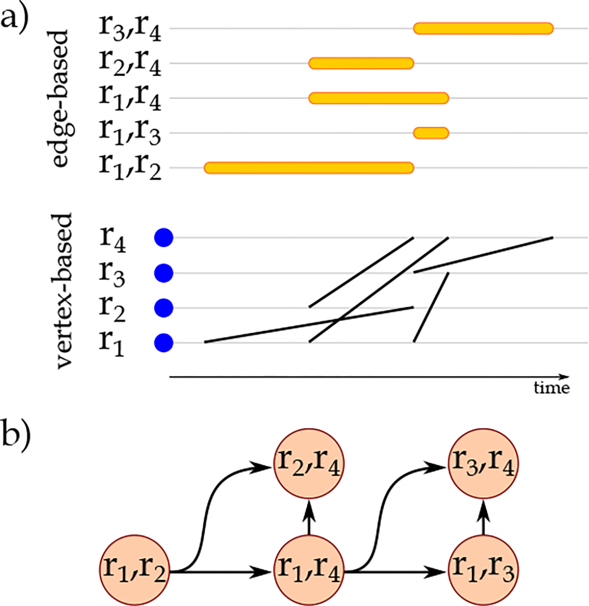
Visualization of physiological and biological biomarkers relationships a) in edge-based and vertex-based representations and b) by the corresponding . In the representation, directed edges connect the nodes that appear sooner to the nodes that appear later (subject to the other conditions of construction). In cases where both nodes appear at the same time, we could connect the nodes with lexicographically smaller labels to the nodes with larger labels and follow an identical approach for all the created in the data set.
For mining frequent patterns in a data set of temporal networks, , we iterate over the networks one by one. For each , one is constructed. Based on the temporal networks in , a data set of is constructed. The tempowork algorithm then mines . To perform the mining, it adopts the depth-first search strategy. Given a frequency threshold , the tempowork output would be a complete set of frequent temporal patterns in appearing in at least networks of the .
The mining process starts with single vertices and edges in the in . The vertices and edges in with frequencies more than are recorded. Note that these vertices and edges represent the frequent edges and frequent subgraphs of size 2 in , respectively. For these frequent patterns, an occurrence list is created, recording the location of their appearance in . Then frequent patterns (parents) are extended using the frequent edges. The frequencies of extended patterns (candidates) are evaluated based on the occurrence list of their corresponding parents. If the number of in the supporting a candidate is more than the frequency threshold , we record as a frequent pattern. Also, we add and locations of its appearances in in the occurrence list. This process is iteratively repeated until no further extension of the frequent patterns is possible. Further details related to this subsection is provided in Appendix B.1.
Algorithm 1.
Frequent Temporal Pattern Mining Algorithm
| 1: | procedure frequent_temporal_pattern_mining() | |
| 2: | Initialize | ▷ An empty set to record associated with temporal networks. |
| 3: | for do | |
| 4: | Initialize with empty vertex and edge sets | |
| 5: | for do | |
| 6: | Add a vertex to corresponding to | |
| 7: | Label in with the endpoints’ and edge’s labels and duration of | |
| 8: | Identify other overlapping edges in read prior to and with vertices in common with and with vertices in common with | |
| 9: | Connect corresponding vertices in to with directed edges | |
| 10: | Label the connections with their starting points’ differences in | |
| 11: | Append to | |
| 12: | frequent_temporal_patterns = PATTERN_MINING() | |
| 13: | Return frequent_temporal_patterns | |
Algorithm 2.
Frequent Pattern Mining Algorithm
| 1: | procedure pattern_mining() |
| 2: | one_vertex: Set of vertices in with frequencies |
| 3: | one_edge: Set of unique edges in with frequencies |
| 4: | frequent_patterns = {one_vertex,one_edge} |
| 5: | procedure frequent_pattern_mining(,candidate) |
| 6: | if is_valid(candidate) then ▷ If candidate is the representative of all the networks isomorphic to candidate. |
| 7: | frequent_pattern ← candidate |
| 8: | Append frequent_pattern to frequentl_patterns |
| 9: | Extend frequent_pattern with edges in one_edge → candidates |
| 10: | for candidate ∈ candidates do |
| 11: | |
| 12: | if then |
| 13: | FREQUENT_PATTERN_MINING(,candidate) |
| 14: | for e ∈ one_edge do FREQUENT_PATTERN_MINING() |
| 15: | Return frequent_patterns |
We use the frequent patterns detected by the tempowork at different frequency thresholds as features to classify and predict sepsis patients. The main goal is to detect patterns that are frequent, shared among a large number of patients, and important enough to be used as differentiating patterns in sepsis versus non-sepsis patients. To identify these frequent and important patterns, we apply different machine learning algorithms to the patterns detected by the tempowork.
3.4. Frequent Evolving Patterns
In addition to using frequent patterns detected in the previous step as features for classification and prediction, we identify the frequent evolution events of physiological and biological biomarkers. As we are using a continuous-time representation of patients’ EHR, we use an extended version of tempowork for mining frequent evolving patterns. This extension of tempowork considers three user-defined thresholds, size parameter , connectivity radius , and continuity radius . These parameters are used to characterize different evolution events. In total, we consider six fundamental evolution events; birth (appearance of a pattern), expansion (continuous growth of a pattern), merge (joining of patterns), contraction (continuous reduction in the size of a pattern), split (transformation of one connected component into two or more connected components), and death (disappearance of a pattern). More descriptive definitions of these events based on parameters , and are provided in Appendix B.2.
Figure 5 visualizes the evolution events considered in this study. For identification of these events, we iterate over the in . For each , we identify the evolution events by checking each vertex, its neighbors, and the connected component that the vertex belongs to, and their temporal changes. In the evolution event identification step, we start with birth and death events. Then, we identify the merge and split events. The expansion and contraction events are identified inside both connected components contributing to the merge and split events and in patterns of physiological and biological biomarkers for which no merge and split events are identified.
Figure 5:

The six fundamental evolution events considered in this study. These events are identified from the associated with temporal networks created based on the relationships among patients’ physiological and biological biomarkers. The vertices contributing to events are shown in different colors.
Algorithm 3.
Frequent Evolving Pattern Mining Algorithm
| 1: | procedure frequent_evolving_pattern_mining() |
| 2: | Initialize as a data set of evolution networks as empty sets for birth, expansion, merge, contraction, split, and death events |
| 3: | for do |
| 4: | Initialize as an empty evolution network |
| 5: | Identify Connected components in |
| 6: | Populate with birth events detected as vertices with in-degree = 0 and all their neighbors in connectivity radius |
| 7: | = Edges ordered based on their starting times in reverse order |
| 8: | Populate with merge events by identification of edges in the order of whose removal increases the number of connected components with size |
| 9: | = Edges ordered based on their finish times |
| 10: | Populate with split events by identification of edges in the order of whose removal increases the number of connected components with size |
| 11: | for do |
| 12: | Populate = with expansion events in |
| 13: | Populate = with contraction events in |
| 14: | for and do |
| 15: | Populate = with expansion events |
| 16: | Populate = with contraction events in |
| 17: | Populate with death events detected as vertices with out-degree = 0 and all their neighbors in connectivity radius |
| 18: | Create evolution network composed of vertices representing by evolution events and edges representing the connections among evolution events based on their component/sub-component relationships |
| 19: | Append to |
| 20: | frequent_evolving_patterns = PATTERN_MINING() |
| 21: | Return frequent_evolving_patterns |
In the next step, the relationships among evolution events identified and their appearance and disappearance time in relation to other events can be used to create an evolution network for the patient. Therefore, we can create a data set of evolution networks corresponding to the temporal changes in patients’ physiological and biological biomarkers. Then, a frequent subgraph mining approach [30] is applied to the data set of evolution networks to identify the most frequent evolving patterns. In this case, we define a frequency threshold to detect the frequent evolving patterns. The pseudocode for identification of evolution events and creation of a data set of evolution networks, , is provided in Algorithm 3. Once is created, it is sent to Algorithm 2 in which the frequent evolving patterns are detected. Note that for both frequent temporal pattern mining and frequent evolving pattern mining, Algorithm 2 is applied to a data set of networks. For the former, the data set of is sent to Algorithm 2. However, for the latter, first, we create the data set of . This data set is sent to Algorithm 3 and the data set of evolution networks, , is created. Then, is passed to the Algorithm 2 for identification of frequent evolving patterns. The function is_valid used in Algorithm 2 has different functionalities when it is applied to and . For , the networks are . To verify the validity of a , first, it is converted to the associated temporal network, and then the temporal network is converted back to a . It is required because, as it is discussed in [33], for each temporal network, we can create only one . However, multiple might represent the same temporal network. This problem is more common in densely connected . As discussed, the edges in represent the delays between nodes’ starting times. The temporal relationships among different nodes can be derived by following different paths over the same . To avoid over-counting these patterns, we need to construct the complete based on the known temporal relationships among nodes and edges. In other words, even though some of the edges might be missing, their presence can be proved based on the known relationships among nodes and the edges in the network. These conversions are performed before the validity of is evaluated to avoid redundancy and over-counting of frequent patterns. On the other hand, when is sent to Algorithm 2, each network is a directed static network, and this conversion is not required. For evaluation of validity, we can use different approaches proposed for canonical labeling of networks [30]. We use the same approach proposed in [34, 35].
The output of this phase would be a data set of temporal evolving patterns. Combined with other feature sets discussed earlier, they are used to classify sepsis and non-sepsis patients.
3.5. Sepsis Onset Prediction
Based on the discussions above, we have three different feature sets; individual responses, frequent temporal patterns, and frequent evolving patterns. Furthermore, we consider patients’ age, gender, and medical history as a separate feature set that can be added to the three previous feature sets. Based on different combinations of feature sets, we develop different machine learning models for the sepsis onset prediction in 3, 6, 12, and 24 hours before sepsis onset. The machine learning algorithms adopted are logistic regression (LG) [36], k-nearest neighbors (kNN) [37], support vector machines with radial basis function (SVM) and polynomial (SVMP) kernels [38], Gaussian Naïve Bayes [39], decision tree (DT) [40] classifiers and two ensemble learning methods; random forest (RF) [41] and Ada Boost Classifier (ADA) [42]. Furthermore, we implemented an imputation approach to handle the missing data. The details of this approach are provided in Appendix B.3.
We used a 10-fold cross-validation approach for training and internal validation for all the predictive models. The training of the predictive models was performed using 70% of the data. All the performance metrics reported in the following sections of the paper are based on a 30% untouched subset of data sets in each iteration used for testing purposes.
For the identification of frequent temporal patterns to be used as features for predictive modeling, we implement tempowork algorithm for different frequency thresholds, temporal noise tolerance threshold, and different types of isomorphism. For identification of evolving patterns, we test different values for size parameter , connectivity radius , and continuity radius . Also, as discussed below, we categorize the labels of nodes. The results of implementing different machine learning algorithms are provided in the next section. Figure 6 visualizes the analytical approach adopted for sepsis onset prediction.
Figure 6:
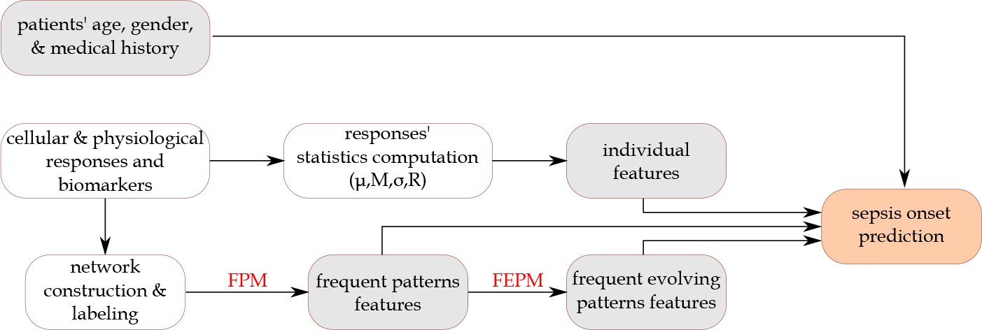
The analytical approach adopted in this study for sepsis onset prediction. The boxes in grey represent the feature sets used. FPM: Frequent pattern mining; FEPM: Frequent evolving pattern mining.
4. Results and Discussion
We applied the approaches described in Section 3 to the study data set. We identified frequent temporal and evolving patterns and used different combinations of these patterns with individual statistics of physiological and biological biomarkers and patients’ age, gender, and medical history for early prediction of sepsis incidence. In the following subsections, we summarize the results obtained corresponding to different approaches discussed in 3.
4.1. Individual Features
From the 19 responses considered in this study, the measurements for 17 responses are provided in numeric values. The measurements are provided in nominal and categorical values for two other responses, Oxygen () source and Glasgow best verbal responses. Therefore, we computed the , , , and for the former responses. We only used the mode for the latter, representing the most common status of the patient for these responses. Based on these considerations, we created 70 features from responses (17 × 4 + 2). In addition, we considered age and gender and 30 different medical complications (as binary features) that patients had experienced in their medical history. The results for sepsis prediction for these feature sets are provided in Table 3. Among the eight prediction models adopted, the SVM and RF performed the best based on accuracy, recall, precision. Therefore, we consider the results obtained by the SVM as the baseline in this paper. The results of all the other algorithms are summarized in Supplementary materials - Table 2.
Table 3:
The mean (standard deviation) of performance metrics of the support vector machine (SVM) algorithm adopted for identification of sepsis patients in the four data sets of the study. The features used are statistics of individual responses (Ind) and their combinations with age, gender, and medical history of patients ().
| Gap (hours) | Features | Accuracy | Recall | Precision |
|---|---|---|---|---|
|
| ||||
| 3 | 0.72 (0.02) | 0.69 (0.03) | 0.70 (0.03) | |
| 0.76 (0.02) | 0.77 (0.02) | 0.72 (0.02) | ||
|
| ||||
| 6 | 0.71 (0.02) | 0.68 (0.03) | 0.69 (0.03) | |
| 0.75 (0.02) | 0.76 (0.02) | 0.71 (0.03) | ||
|
| ||||
| 12 | 0.71 (0.02) | 0.69 (0.03) | 0.70 (0.03) | |
| 0.75 (0.02) | 0.76 (0.02) | 0.72 (0.03) | ||
|
| ||||
| 24 | 0.68 (0.02) | 0.65 (0.03) | 0.68 (0.04) | |
| 0.73 (0.02) | 0.74 (0.04) | 0.71 (0.03) | ||
4.2. Frequent Temporal Patterns
The tempowork algorithm was applied to the data sets of temporal networks created from patients’ hospitalization courses (3, 6, 12, 24 hours) before the sepsis onset. For each of the network data sets, we considered multiple frequency thresholds. We considered a pattern frequent if it is observed in at least patients . Other parameters that can be tuned in these experiments are isomorphism types (four types) and the level of noise tolerance when inexact versions of isomorphism are adopted. We consider four values for noise tolerance (1, 2, 3, and 4 hours). These values determine how long two measurements are considered inexactly equal if the measurements of the corresponding response are equal, but their duration is different. Implementing the algorithm for the exact time versions of isomorphism showed that it is very rare to find identical frequent patterns with exactly identical duration or exactly identical delays between two responses interactions (even for ). The results related to the number and size of frequent temporal patterns detected from different data sets and for two isomorphism definitions at different support thresholds are provided in Appendix C. This appendix also includes the results related to the number and size of frequent temporal patterns detected from the data sets with 3-hour window for different temporal noise tolerance thresholds, numbers of labeling categories and the two isomorphism definitions at different support threshold.
4.3. Frequent Evolving Patterns
The constructed based on patients’ physiological and biological biomarkers in different data sets of the study are used to identify evolution events and create the evolution networks. For this purpose, different values for size parameter , connectivity radius , and continuity radius are tried. In addition, we used different frequency thresholds to detect frequent evolving patterns. A modified version of the approach proposed in [34, 35, 43] is used for the identification of evolving patterns in the data set of evolution networks. Figure 7 shows the number of frequent patterns detected for for different values of , , , and . The results obtained for different data sets are shown and compared in Supplementary materials - Figure 5.
Figure 7:
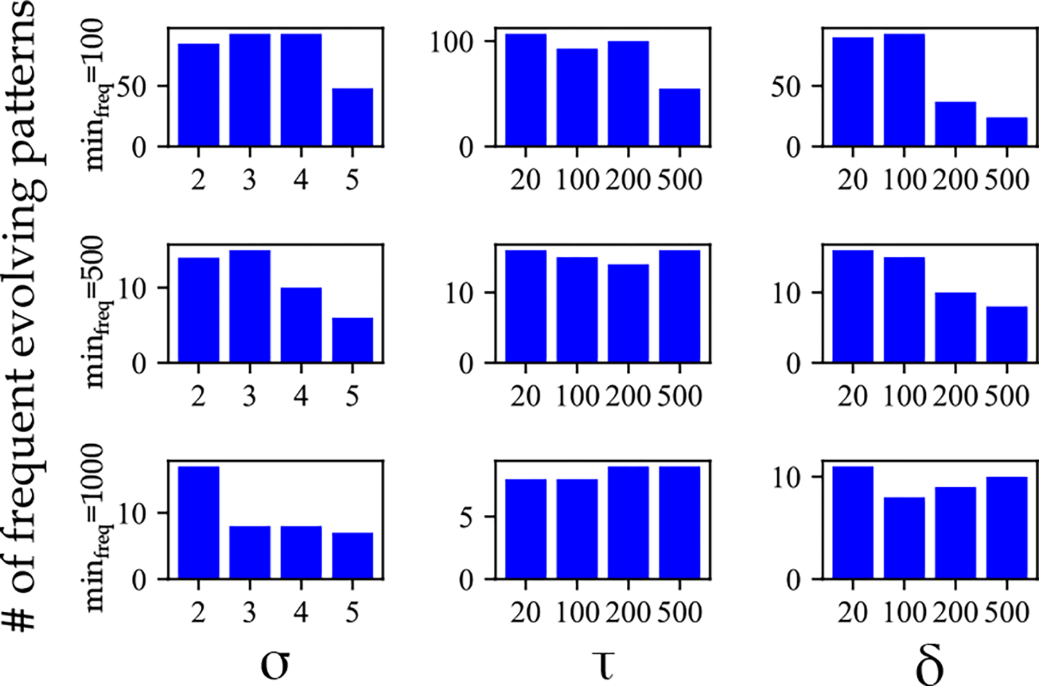
The number of frequent evolving patterns identified in the data set of the study for different values of parameters , , , and .
4.4. Sepsis Onset Prediction
Different combinations of individual features, frequent patterns, and frequent evolving patterns with and without age, gender, and medical history of patients were used for sepsis onset prediction. The frequent temporal patterns and frequent evolving patterns are used as binary features. For each patient, it takes a value of 1 if observed in the patient’s hospitalization records. The results of predictive modeling for the SVM models for two different isomorphism definitions are provided in Figure 8. Considering that the inexact sequence-preserved isomorphism produced the best performance, the results for all the algorithms and different periods before sepsis onset are provided in Supplementary materials (Table 2 and Figure 1). The performance of the SVM algorithm for different feature sets and support values are provided in Figure 9.
Figure 8:
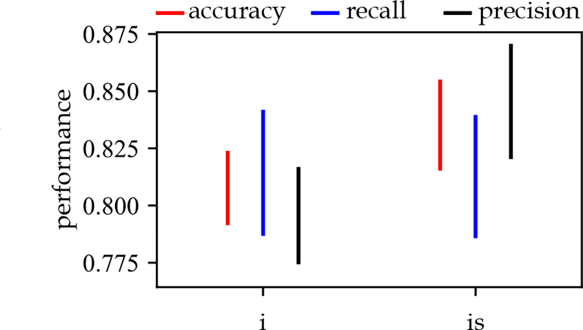
The performance of the SVM algorithm for two different definitions of isomorphism. : inexact-time isomorphism, : inexact-time sequence-preserved isomorphism in combination with all other feature sets.
Figure 9:
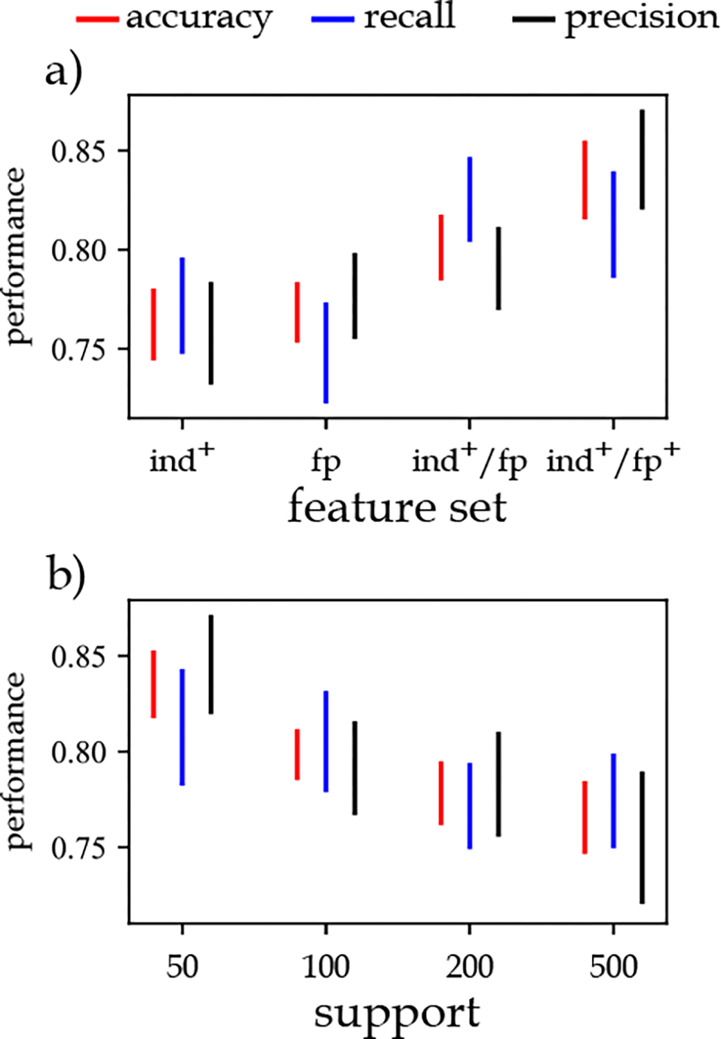
The impact of a) different feature sets and b) support values for sepsis onset prediction. : statistics of individual responses, and patients’ age, gender, and medical history, : frequent temporal patterns, : statistics of individual responses, and patients’ age, gender, and medical history, and frequent temporal patterns, : statistics of individual responses, and patients’ age, gender, and medical history, frequent temporal patterns, and frequent evolving temporal patterns.
Considering that adopting is isomorphism definition produces a large number of frequent patterns, we used a supervised feature selection approach. The results showed that selecting the 1000 most important features based on the feature selection approach almost always produces the best results for the combination of accuracy, recall, and precision performance metrics (refer to Supplementary materials). Based on these findings, we conducted a series of experiments to identify the best combination of features, support thresholds, temporal noise tolerance threshold, and the number of labeling categories.
The results (Figure 9.a) showed that using the statistics of individual responses , combined with age, gender, and medical history of patients as one feature set results in an accuracy of about 76%. Using only frequent patterns produced slightly better results than the feature set. When we combine these two feature sets , the accuracy increases by about 3–4%. Adding the frequent evolving patterns to the previous feature sets further improves these performance metrics by about 2–3%.
We also found that the highest performance is obtained at the support threshold (Figure 9.b). It implies that by increasing the support threshold, we remove some of the patterns considered frequent at lower thresholds. These patterns have a role in differentiating sepsis and non-sepsis patients. The results show that at frequency threshold and , the classification performance is almost equal to the case where the feature set comprises features related to the statistics of individual responses, age, gender, and medical history of patients. It means that frequent patterns (and evolving patterns) detected at these frequency thresholds are common in both sepsis and non-sepsis patients. Therefore, they cannot be used to differentiate these two subpopulations effectively.
Furthermore, we can rank features based on their importance in classifying patients into sepsis and non-sepsis subpopulations. We categorized the top ten most important features in the four categories of i) statistics of physiological and biological biomarkers, ii) features related to age, gender, and medical history of patients, iii) frequent temporal patterns, and iv) frequent evolving patterns. The ranking was performed using univariate statistical tests based on the ANOVA F-value scoring function [44]. Table 4 lists the top ten most important features in the first feature set. This table shows that fluctuations in platelet, lactate, and creatinine (represented by the range and standard deviation statistics) are among the top ten most important features. On the other hand, the mean and median of systolic blood pressure and oxygen source mode are considered important features for this classification problem.
Table 4:
The ten most important statistics of physiological and biological biomarkers and biomarkers ordered by their importance rank in the classification of sepsis and non-sepsis patients. SD: Standard deviation, WBC: White blood cells count.
| feature | rank in set | rank in all |
|---|---|---|
|
| ||
| Range of platelet | 1 | 2 |
| Mean of systolic blood pressure | 2 | 4 |
| Mode of oxygen source | 3 | 5 |
| Median of systolic blood pressure | 4 | 6 |
| SD of platelet | 5 | 7 |
| SD of lactate | 6 | 8 |
| Range of lactate | 7 | 9 |
| Range of creatinine | 8 | 10 |
| Range of WBC | 9 | 32 |
| SD of creatinine | 10 | 38 |
The most important feature identified in the classification problem belongs to the feature set related to age, gender, and medical history of patients; electrolyte disorders (Table 5). The second most important feature in this group and the third most important feature among all the features is significant weight-loss in the history of patients. The patients’ gender is also an important feature in this group. However, the age of patients is not identified in the top ten most important features in this feature set.
Table 5:
The ten most important features related to age, gender, and medical history of patients ordered by their importance rank in the classification of sepsis and non-sepsis patients.
| feature | rank in set | rank in all |
|---|---|---|
|
| ||
| Electrolyte disorders | 1 | 1 |
| Significant weight-loss | 2 | 3 |
| Anemic disorders | 3 | 11 |
| Coagulation disorders | 4 | 29 |
| Chronic pulmonary disease | 5 | 31 |
| Paralysis prior to this visit | 6 | 32 |
| Diabetes | 7 | 49 |
| Peripheral vascular disease | 8 | 77 |
| Gender | 9 | 101 |
| Depression | 10 | 149 |
Figure 10 shows the most important features in the group of frequent patterns. As provided in the code next to each frequent pattern (second placeholder), none of the frequent patterns are among the top 10 most important features for classification. It means that none of these features can individually differentiate a large number of sepsis patients from non-sepsis patients compared to the two other feature sets. However, as there are many frequent patterns detected by the algorithm in this study, each of them (or their combination) can differentiate some of the patients and improve the classification problem performance. Except for the oxygen source, for all the other vertices in this figure, a label is provided in the form of “xxxx”. These codes are concatenation of statistics. Because the classification is conducted with two labeling categories for each statistic, 1 in these codes means that the corresponding vertex has a high value for the corresponding statistics, 0 otherwise. In other words, for example, 1101 for the bilirubin means that a temporal pattern of bilirubin lasting between 4 to 8 hours, with high , high , low , and high has been identified as a frequent pattern.
Figure 10:
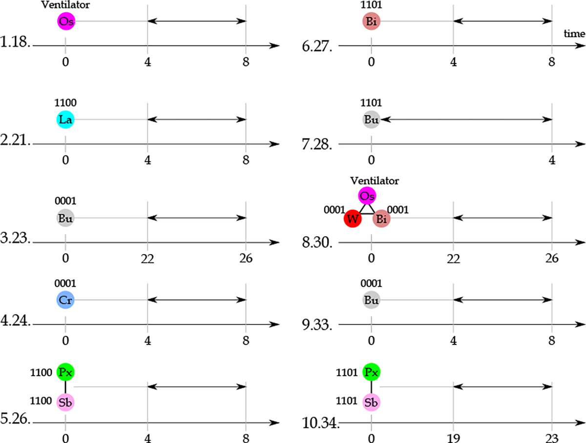
The ten most important frequent patterns in the classification of sepsis and non-sepsis patients. Next to each pattern, a code is provided representing the importance rank of the pattern in the feature set composed of frequent temporal patterns and their importance rank in the entire feature set. The duration of the temporal pattern is shown with black arrows. For the explanation related to code associated with each vertex, refer to the text. Bi: BiliRubin, Bu: BUN, Cr: Creatinine, La: Lactate, Os: Oxygen source, Px: Pulse ox, Sb: Systolic blood pressure, W: White blood cells count.
Figure 11 shows the ten most important features in frequent evolving patterns. The results show that this set of features are generally more important than frequent patterns. This difference in importance can be attributed to the frequent evolving pattern being considered a generalization of frequent temporal patterns, as different temporal patterns might map to the same evolving patterns. Another observation made was that most of the important frequent evolving patterns shown in Figure 11 include an expansion, or merge, or both of these two events (compared to contraction or split events). These events are associated with the increasing number of physiological and biological biomarkers measurements, representing closer examinations of the patients experiencing more severe conditions.
Figure 11:
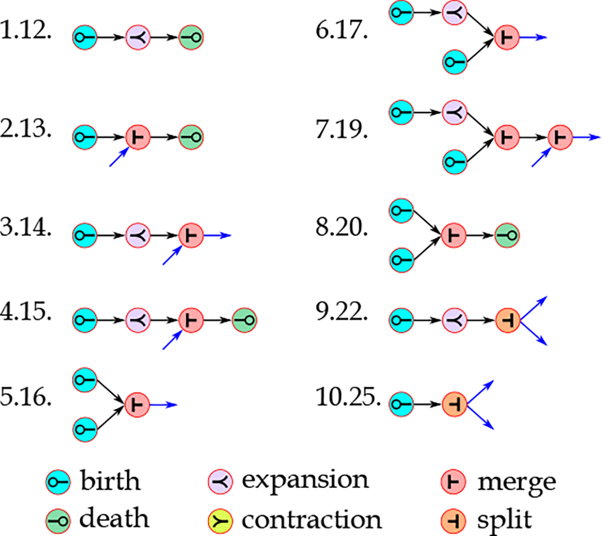
The ten most important frequent evolving patterns in the classification of sepsis and nonsepsis patients. The frequent evolving pattern mining approach has not detected the blue edges. However, they are shown to emphasize that these events should be connected to other events by their definition, and they are not shown as they have not been frequent. Next to each pattern, a code is provided representing the importance rank of the pattern in the feature set composed of frequent evolving patterns and their importance rank in the entire feature set.
Although, in most cases, a combination of features contributes to differentiating sepsis from nonsepsis patients, we could identify the evolution events and patterns frequently appearing in sepsis patients. We found that patients showing one or multiple instances of the patterns shown in Figure 12 are more likely to become sepsis patients. We observed that these patterns (events) either contribute to the appearance of multiple physiological and biological biomarkers through the birth event or the increase in the size of the patterns through expansion or merge events. We also observed that these patterns are composed of co-appearances of more severe conditions of responses associated with two or more than two organ systems (shown with different colors in Figure 12). This observation highlights the importance of considering the changes in multiple organ systems’ rather than isolated individual organ systems. Another observation was that in many of these patterns, the responses associated with the renal organ system represented by creatinine (Cr) or BUN (Bu) and metabolic organ system represented by lactate (La) are more common than other organ systems.
Figure 12:
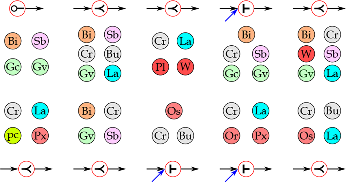
The ten most common evolution events observed among sepsis patients with the lowest frequencies among non-sepsis patients. The responses representing the same organ system are shown with the same color (Bi: Bilirubin; Bu: BUN; Cr: Creatinine; Gc: Glasgow Coma Score; Gv: Glasgow Best Verbal Response; La: Lactate; Or: ; Os: Oxygen Source; pc: Procalcitonin; Pl: Platelet; Px: Pulse oximetry (); Sb: systolic blood pressure; W: WBC), ⟜ : birth, ≺ : expansion, ⊢ : merge).
There are many studies in the sepsis literature devoted to improving the early prediction of sepsis onset as it is known that successful prediction of sepsis incidence can significantly improve the patients’ outcomes. Furthermore, the interpretability of analytical approaches’ findings in clinical settings can promote the adoption of these approaches. Consequently, the investigation of model explain-ability and interpretability of findings in clinical settings has attracted increasing attention in recent years. This study aimed to propose an approach to improve the prediction of sepsis onset using interpretable feature sets. With the proposed methods in this study, we could identify the most important features contributing to the patients’ classification. These features are either simple statistics of individual responses, patients’ medical history, or temporal dynamics and evolution of physiological and biological biomarkers as shown in Figures 10, 11, and 12. The importance of all these components can be clinically verified. Using graph matching approaches for any patient of interest, we could retrieve similar patients to the patient of interest using a vector of important features and components. As a result, we can enhance the clinical interpretability of findings by using a diverse set of features and incorporating the temporal changes in patients’ states.
5. Conclusion
In this paper, we used a frequent temporal pattern mining approach to identify frequent patterns in populations of sepsis patients. We showed that using these patterns can improve the prediction performance of sepsis onset. The investigation of different combinations of feature sets revealed that although the individual features (the typical approach in the literature) and frequent patterns identified have almost identical performance for predicting sepsis onset, their combination can further improve the performance. It implies that the recurring patterns probably carry a different type of information that cannot be captured by the statistics used in this study to represent the average values and fluctuations of physiological and biological biomarkers. In many decision applications, decision-makers act upon individual observations to start, stop, or change treatment strategies. However, our results showed that individual responses have limited value and power compared to when a rich repository of both individual responses and frequent temporal or evolving patterns is the source of decision making.
Nevertheless, this study has some limitations. First, the data used in this study is from one health care system. The reliability of results should be investigated by applying the same approach to data sets from different health care systems. Furthermore, to evaluate the robustness of the proposed algorithms, we would like to apply them to real-world data sets related to other health conditions. It is an avenue for our future work.
The main objectives of this paper were to show the importance of consideration of temporality in the feature engineering phase for early sepsis prediction and propose an approach to enhance the interpretability of the findings. Therefore, we adopted a balanced data set with a specific experimental design and used traditional machine learning algorithms. Although sepsis is a prevalent health complication, adopting a balanced data set is still an overestimated number of sepsis incidences. Furthermore, the evaluation of patients for identification of sepsis incidence starts with and is continuously monitored after the hospitalization. However, the experimental design and patient inclusion criteria adopted in this work (Figure 1) is a simplified version of the sepsis identification problem in real-world settings. Therefore, adopting methods specifically developed for imbalanced data sets (e.g., refer to [45, 46, 47]) with the same types of features proposed in this study might be beneficial. Although the frequent temporal and evolving patterns common among sepsis patients can be mined from already collected sepsis patients’ data sets, the identification of these patterns in patients in hospitalization should be continuously performed. Furthermore, the algorithms adopted in this study are mainly traditional machine learning algorithms. The usefulness of the feature sets developed in this study can be examined with more advanced deep learning approaches for better performance. We could not apply these approaches in this study because of the limited data sets (and the large number of frequent patterns detected). Also, although we could capture the temporal aspects of physiological and biological biomarkers, we still used summary statistics to represent their values and dynamics. In our future work, we are interested in developing models that capture these characteristics of data entirely.
In this study, first, we identified the frequent patterns and then used supervised feature selection and classification approaches to identify the most important features. In addition to working on the limitations above, we would like to integrate the frequent temporal mining approach with the classification algorithm into one step. This integration can enhance the efficiency of the proposed approach by eliminating frequent patterns whose growth does not seem promising and therefore limit the search space as early as possible.
Supplementary Material
Using frequent temporal patterns can improve the performance of sepsis onset prediction.
The patients with more severe renal and metabolic organ systems’ manifestations are more likely to be sepsis patients.
The identification of critical temporal patterns contributing to the prediction performance improves clinical interpretability.
The rich repository of frequent temporal and evolving patterns can inform personalized treatment and management of sepsis.
Acknowledgment
We would like to acknowledge that this work has been performed on behalf of the Sepsis Early Prediction Support Implementation System Collaborative. This work was supported by the National Science Foundation Smart and Connected Health (Award Number: 1833538) and the National Library of Medicine of the National Institutes of Health (Grant Number: 1R01LM012300-01A1, Award Number: R01LM012300). This work was also supported in part by the National Science Foundation under the Grant NSF-1741306, IIS-1650531, and DIBBs-1443019. Any opinions, findings, and conclusions or recommendations expressed in this material are those of the author(s) and do not necessarily reflect the views of the National Science Foundation.
Footnotes
Declaration of interests
The authors declare that they have no known competing financial interests or personal relationships that could have appeared to influence the work reported in this paper.
Publisher's Disclaimer: This is a PDF file of an unedited manuscript that has been accepted for publication. As a service to our customers we are providing this early version of the manuscript. The manuscript will undergo copyediting, typesetting, and review of the resulting proof before it is published in its final form. Please note that during the production process errors may be discovered which could affect the content, and all legal disclaimers that apply to the journal pertain.
Bibliography
- [1].Singer Mervyn et al. “The Third International Consensus Definitions for Sepsis and Septic Shock (Sepsis-3)”. In: JAMA 315.8 (Feb. 2016), pp. 801–810. ISSN: 0098–7484. DOI: 10.1001/jama.2016.0287. [DOI] [PMC free article] [PubMed] [Google Scholar]
- [2].Rudd Kristina E et al. “Global, regional, and national sepsis incidence and mortality, 1990–2017: analysis for the Global Burden of Disease Study”. In: The Lancet 395.10219 (2020), pp. 200–211. ISSN: 0140–6736. DOI: 10.1016/S0140-6736(19)32989-7. [DOI] [PMC free article] [PubMed] [Google Scholar]
- [3].Torio Celeste M and Andrews Roxanne M. “National Inpatient Hospital Costs: The Most Expensive Conditions by Payer, 2011: Statistical Brief #160”. In: Healthcare Cost and Utilization Project (HCUP) Statistical Briefs (2013). url: https://www.ncbi.nlm.nih.gov/books/NBK169005/.
- [4].Rhee Chanu et al. “Prevalence, Underlying Causes, and Preventability of Sepsis-Associated Mortality in US Acute Care Hospitals”. In: JAMA Network Open 2.2 (Feb. 2019), e187571–e187571. ISSN: 2574–3805. DOI: 10.1001/jamanetworkopen.2018.7571. [DOI] [PMC free article] [PubMed] [Google Scholar]
- [5].Gultepe Eren et al. “From vital signs to clinical outcomes for patients with sepsis: A machine learning basis for a clinical decision support system”. English (US). In: Journal of the American Medical Informatics Association : JAMIA 21.2 (2014), pp. 315–325. ISSN: 1067–5027. DOI: 10.1136/amiajnl-2013-001815. [DOI] [PMC free article] [PubMed] [Google Scholar]
- [6].Horng Steven et al. “Creating an automated trigger for sepsis clinical decision support at emergency department triage using machine learning”. In: PLOS ONE 12.4 (Apr. 2017), pp. 1–16. DOI: 10.1371/journal.pone.0174708. [DOI] [PMC free article] [PubMed] [Google Scholar]
- [7].Shimabukuro David W et al. “Effect of a machine learning-based severe sepsis prediction algorithm on patient survival and hospital length of stay: a randomised clinical trial”. In: BMJ Open Respiratory Research 4.1 (2017). DOI: 10.1136/bmjresp-2017-000234. [DOI] [PMC free article] [PubMed] [Google Scholar]
- [8].Nemati Shamim et al. “An interpretable machine learning model for accurate prediction of sepsis in the ICU”. In: Critical care medicine 46.4 (2018), p. 547. [DOI] [PMC free article] [PubMed] [Google Scholar]
- [9].Javed Adnan et al. “Clinical predictors of early death from sepsis”. In: Journal of Critical Care 42 (2017), pp. 30–34. ISSN: 0883–9441. DOI: 10.1016/j.jcrc.2017.06.024. [DOI] [PMC free article] [PubMed] [Google Scholar]
- [10].Calvert Jacob S. et al. “A computational approach to early sepsis detection”. In: Computers in Biology and Medicine 74 (2016), pp. 69–73. ISSN: 0010–4825. DOI: 10.1016/j.compbiomed.2016.05.003. [DOI] [PubMed] [Google Scholar]
- [11].Larsen Frederik Fruergaard and Petersen J. Asger. “Novel biomarkers for sepsis: A narrative review”. In: European Journal of Internal Medicine 45 (2017). Special Issue: Acutely Ill Patients, pp. 46–50. ISSN: 0953–6205. DOI: 10.1016/j.ejim.2017.09.030. [DOI] [PubMed] [Google Scholar]
- [12].Henriquez-Camacho Cesar and Losa Juan. “Biomarkers for Sepsis”. In: BioMed Research International 2014 (2014). DOI: 10.1155/2014/547818. [DOI] [PMC free article] [PubMed] [Google Scholar]
- [13].Vincent J-L et al. “The SOFA (Sepsis-related Organ Failure Assessment) score to describe organ dysfunction/failure”. In: IntensiveCare Medicine 22.7 (1996), 707–710. DOI: 10.1007/BF01709751. [DOI] [PubMed] [Google Scholar]
- [14].Rubulotta Francesca et al. “Predisposition, insult/infection, response, and organ dysfunction: A new model for staging severe sepsis”. In: Critical care medicine 37.4 (2009), pp. 1329–1335. DOI: doi: 10.1097/CCM.0b013e31819d5db1. [DOI] [PubMed] [Google Scholar]
- [15].Seymour Christopher W. et al. “Assessment of Clinical Criteria for Sepsis: For the Third International Consensus Definitions for Sepsis and Septic Shock (Sepsis-3)”. In: JAMA 315.8 (Feb. 2016), pp. 762–774. ISSN: 0098–7484. DOI: 10.1001/jama.2016.0288. [DOI] [PMC free article] [PubMed] [Google Scholar]
- [16].Mohaimenul Islam Md et al. “Prediction of sepsis patients using machine learning approach: A meta-analysis”. In: Computer Methods and Programs in Biomedicine 170 (2019), pp. 1–9. ISSN: 0169–2607. DOI: 10.1016/j.cmpb.2018.12.027. [DOI] [PubMed] [Google Scholar]
- [17].Xi Hang Cao Ivan Stojkovic, and Obradovic Zoran. “Predicting sepsis severity from limited temporal observations”. In: International Conference on Discovery Science, Lecture Notes in Computer Science. Springer. 2014, pp. 37–48. [Google Scholar]
- [18].Khoshnevisan Farzaneh et al. “Recent Temporal Pattern Mining for Septic Shock Early Prediction”. In: 2018 IEEE International Conference on Healthcare Informatics (ICHI). 2018, pp. 229–240. DOI: 10.1109/ICHI.2018.00033. [Google Scholar]
- [19].Saqib Mohammed, Sha Ying, and Wang May D.. “Early Prediction of Sepsis in EMR Records Using Traditional ML Techniques and Deep Learning LSTM Networks ”. In: 2018 40th Annual International Conference of the IEEE Engineering in Medicine and Biology Society (EMBC). 2018, pp. 4038–4041. DOI: 10.1109/EMBC.2018.8513254. [DOI] [PubMed] [Google Scholar]
- [20].Moor Michael et al. “Temporal convolutional networks and dynamic time warping can drastically improve the early prediction of sepsis”. In: arXiv preprint arXiv:1902.01659 (2019). [Google Scholar]
- [21].Bedoya Armando D et al. “Machine learning for early detection of sepsis: an internal and temporal validation study”. In: JAMIA Open 3.2 (Apr. 2020), pp. 252–260. ISSN: 2574–2531. DOI: 10.1093/jamiaopen/ooaa006. [DOI] [PMC free article] [PubMed] [Google Scholar]
- [22].Kok Christopher et al. “Automated prediction of sepsis using temporal convolutional network”. In: Computers in Biology and Medicine 127 (2020), p. 103957. ISSN: 0010–4825. DOI: 10.1016/j.compbiomed.2020.103957. [DOI] [PubMed] [Google Scholar]
- [23].Došilović Filip Karlo, Brčić Mario, and Hlupić Nikica. “Explainable artificial intelligence: A survey”. In: 2018 41st International Convention on Information and Communication Technology, Electronics and Microelectronics (MIPRO). 2018, pp. 0210–0215. DOI: 10.23919/MIPRO.2018.8400040. [DOI] [Google Scholar]
- [24].Gilpin Leilani H. et al. “Explaining Explanations: An Overview of Interpretability of Machine Learning”. In: 2018 IEEE 5th International Conference on Data Science and Advanced Analytics (DSAA). 2018, pp. 80–89. DOI: 10.1109/DSAA.2018.00018. [Google Scholar]
- [25].Adadi Amina and Berrada Mohammed. “Explainable AI for Healthcare: From Black Box to Interpretable Models”. eng. In: Embedded Systems and Artificial Intelligence. Advances in Intelligent Systems and Computing. Singapore: Springer Singapore, 2020, pp. 327–337. isbn: 9789811509469. [Google Scholar]
- [26].Vellido Alfredo. “The importance of interpretability and visualization in machine learning for applications in medicine and health care”. In: Neural computing and applications (2019), pp. 1–15. DOI: 10.1007/s00521-019-04051-w. [DOI] [Google Scholar]
- [27].Jazayeri Ali et al. “Network-Based Modeling of Sepsis: Quantification and Evaluation of Simultaneity of Organ Dysfunctions”. In: Proceedings of the 10th ACM International Conference on Bioinformatics, Computational Biology and Health Informatics. BCB ‘19. Niagara Falls, NY, USA: Association for Computing Machinery, 2019, 87–96. ISBN: 9781450366663. DOI: 10.1145/3307339.3342160. [Google Scholar]
- [28].Jazayeri Ali et al. “Proximity of Cellular and Physiological Response Failures in Sepsis”. In: IEEE Journal of Biomedical And Health Informatics (2021), in press. [DOI] [PubMed] [Google Scholar]
- [29].da Fontoura Costa Luciano et al. “Analyzing and modeling real-world phenomena with complex networks: a survey of applications”. In: Advances in Physics 60.3 (2011), pp. 329–412. DOI: 10.1080/00018732.2011.572452. [DOI] [Google Scholar]
- [30].Jazayeri Ali and Yang Chris. “Frequent Subgraph Mining Algorithms in Static and Temporal Graph-Transaction Settings: A Survey”. In: IEEE Transactions on Big Data (2021). DOI: 10.1109/TBDATA.2021.3072001. [DOI] [Google Scholar]
- [31].Rhee Chanu et al. “Incidence and trends of sepsis in US hospitals using clinical vs claims data, 2009–2014”. In: JAMA 318.13 (Oct. 2017), pp. 1241–1249. ISSN: 0098–7484. DOI: 10.1001/jama.2017.13836. [DOI] [PMC free article] [PubMed] [Google Scholar]
- [32].Jazayeri Ali and Yang Christopher C. “Motif discovery algorithms in static and temporal networks: A survey”. In: Journal of Complex Networks 8.4 (Dec. 2020). cnaa031. ISSN: 2051–1329. DOI: 10.1093/comnet/cnaa031. url: 10.1093/comnet/cnaa031. [DOI] [Google Scholar]
- [33].Jazayeri Ali and Yang Christopher C.. Frequent Pattern Mining in Continuous-time Temporal Networks. 2021. arXiv: 2105.06399 [cs.SI]. [DOI] [PubMed] [Google Scholar]
- [34].Yan Xifeng and Han Jiawei. “gSpan: graph-based substructure pattern mining”. In: 2002 IEEE International Conference on Data Mining, 2002. Proceedings. 2002, pp. 721–724. DOI: 10.1109/ICDM.2002.1184038. [Google Scholar]
- [35].Yan Xifeng and Han Jiawei. Span: graph-based substructure pattern mining. Tech. rep. UIUCDCS-R-2002–2296. University of Illinois at Urbana-Champaign, 2002. [Google Scholar]
- [36].Anzai Yuichiro. Pattern recognition and machine learning. Elsevier, 2012. [Google Scholar]
- [37].Fix Evelyn and Hodges JL. “Discriminatory Analysis. Nonparametric Discrimination: Consistency Properties”. In: International Statistical Review / Revue Internationale de Statistique 57.3 (1989), pp. 238–247. ISSN: 03067734, 17515823. url: http://www.jstor.org/stable/1403797. [Google Scholar]
- [38].Suykens Johan AKand Vandewalle Joos. “Least squares support vector machine classifiers”. In: Neural processing letters 9.3 (1999), pp. 293–300. [Google Scholar]
- [39].John George H. and Langley Pat. Estimating Continuous Distributions in Bayesian Classifiers. 2013. arXiv: 1302.4964 [cs.LG]. [Google Scholar]
- [40].Wu Xindong et al. “Top 10 algorithms in data mining”. In: Knowledge and information systems 14.1 (2008), pp. 1–37. DOI: 10.1007/s10115-007-0114-2. [DOI] [Google Scholar]
- [41].Ho Tin Kam. “Random decision forests”. In: Proceedings of 3rd International Conference on Document Analysis and Recognition. Vol. 1. 1995, 278–282 vol.1. DOI: 10.1109/ICDAR.1995.598994. [Google Scholar]
- [42].Freund Yoav and Schapire Robert E. “A Decision-Theoretic Generalization of On-Line Learning and an Application to Boosting”. In: Journal of Computer and System Sciences 55.1 (1997), pp. 119–139. ISSN: 0022–0000. DOI: 10.1006/jcss.1997.1504. [DOI] [Google Scholar]
- [43].Yan Xifeng and Han Jiawei. “CloseGraph: Mining Closed Frequent Graph Patterns”. In: Proceedings of the Ninth ACM SIGKDD International Conference on Knowledge Discovery and Data Mining. KDD ‘03. Washington, D.C.: Association for Computing Machinery, 2003, 286–295. ISBN: 1581137370. DOI: 10.1145/956750.956784. URL: 10.1145/956750.956784. [DOI] [Google Scholar]
- [44].Pedregosa F et al. “Scikit-learn: Machine Learning in Python”. In: Journal of Machine Learning Research 12 (2011), pp. 2825–2830. [Google Scholar]
- [45].Abromavičius Vytautas et al. “Two-Stage Monitoring of Patients in Intensive Care Unit for Sepsis Prediction Using Non-Overfitted Machine Learning Models”. In: Electronics 9.7 (2020). ISSN: 2079–9292. DOI: 10.3390/electronics9071133. URL: https://www.mdpi.com/2079-9292/9/7/1133. [DOI] [Google Scholar]
- [46].Lyra Simon, Leonhardt Steffen, and Antink Christoph Hoog. “Early Prediction of Sepsis Using Random Forest Classification for Imbalanced Clinical Data”. In: 2019 Computing in Cardiology (CinC). 2019, pp. 1–4. DOI: 10.23919/CinC49843.2019.9005769.32514409 [DOI] [Google Scholar]
- [47].Baniasadi Atefeh et al. “Two-Step Imputation and AdaBoost-Based Classification for Early Prediction of Sepsis on Imbalanced Clinical Data”. In: Critical care medicine 49.1 (2020), e91–e97. DOI: 10.1097/CCM.0000000000004705. [DOI] [PubMed] [Google Scholar]
- [48].Jazayeri Ali, Liang Ou Stella, and Yang Christopher C. “Imputation of Missing Data in Electronic Health Records Based on Patients’ Similarities”. In: Journal of Healthcare Informatics Research 4.3 (2020), pp. 295–307. DOI: 10.1007/s41666-020-00073-5. [DOI] [PMC free article] [PubMed] [Google Scholar]
Associated Data
This section collects any data citations, data availability statements, or supplementary materials included in this article.


