Registration for Exponential Family Functional Data

Summary.

We introduce a novel method for separating amplitude and phase variability in exponential family functional data. Our method alternates between two steps: the first uses generalized functional principal components analysis to calculate template functions, and the second estimates smooth warping functions that map observed curves to templates. Existing approaches to registration have primarily focused on continuous functional observations, and the few approaches for discrete functional data require a pre-smoothing step; these methods are frequently computationally intensive. In contrast, we focus on the likelihood of the observed data and avoid the need for preprocessing, and we implement both steps of our algorithm in a computationally efficient way. Our motivation comes from the Baltimore Longitudinal Study on Aging, in which accelerometer data provides valuable insights into the timing of sedentary behavior. We analyze binary functional data with observations each minute over 24 hours for 592 participants, where values represent activity and inactivity. Diurnal patterns of activity are obscured due to misalignment in the original data but are clear after curves are aligned. Simulations designed to mimic the application indicate that the proposed methods outperform competing approaches in terms of estimation accuracy and computational efficiency. Code for our method and simulations is publicly available.

1. Introduction

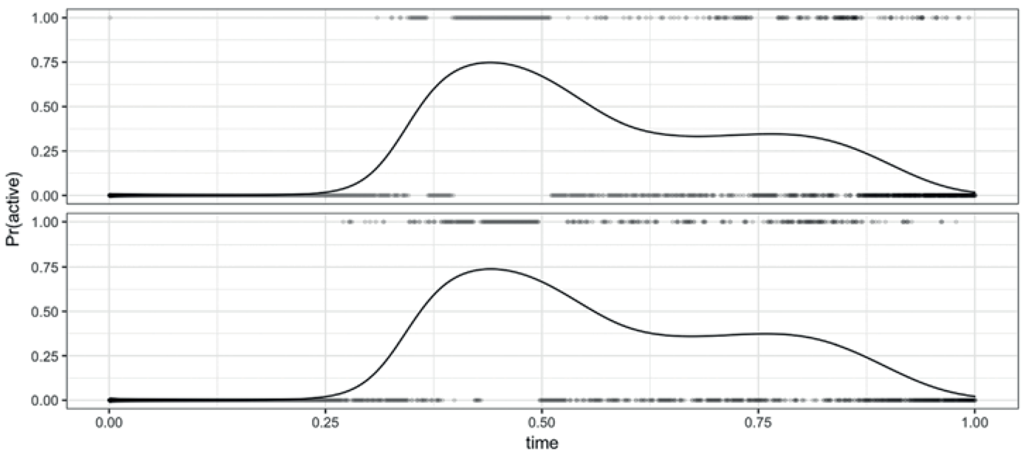
In the most common setting for functional data analysis, the basic unit of observation is the real-valued curve $Y_i(t)$ for subjects $i\in 1,\dots ,N$. More recently, there has been interest in exponential family functional data, where $Y_i(t)$ comes from a non-Gaussian distribution; it is typically assumed that $Y_i(t)$ has a smooth and continuous latent mean, ${\mu }_i(t)=E\left\{Y_i(t)\right\}$. Our motivation is the study of activity and inactivity using data collected with accelerometers, a setting with binary functional data. Figure 1 shows binary curves $Y_i(t)$ for two participants taking the value 1 when the participant is active and 0 when the participant is inactive. A solid curve shows an estimate of the smooth latent mean ${\mu }_i(t)$, interpreted as the probability the subject will be active at each minute in the 24 hours of observation. Other recent examples of non-Gaussian functional data include agricultural studies on the feeding behavior of pigs, spectral backscatter from long range infrared light detection, and longitudinal studies of drug use (Serban et al., 2013; Huang et al., 2014; Gertheiss et al., 2015).

Figure 1.

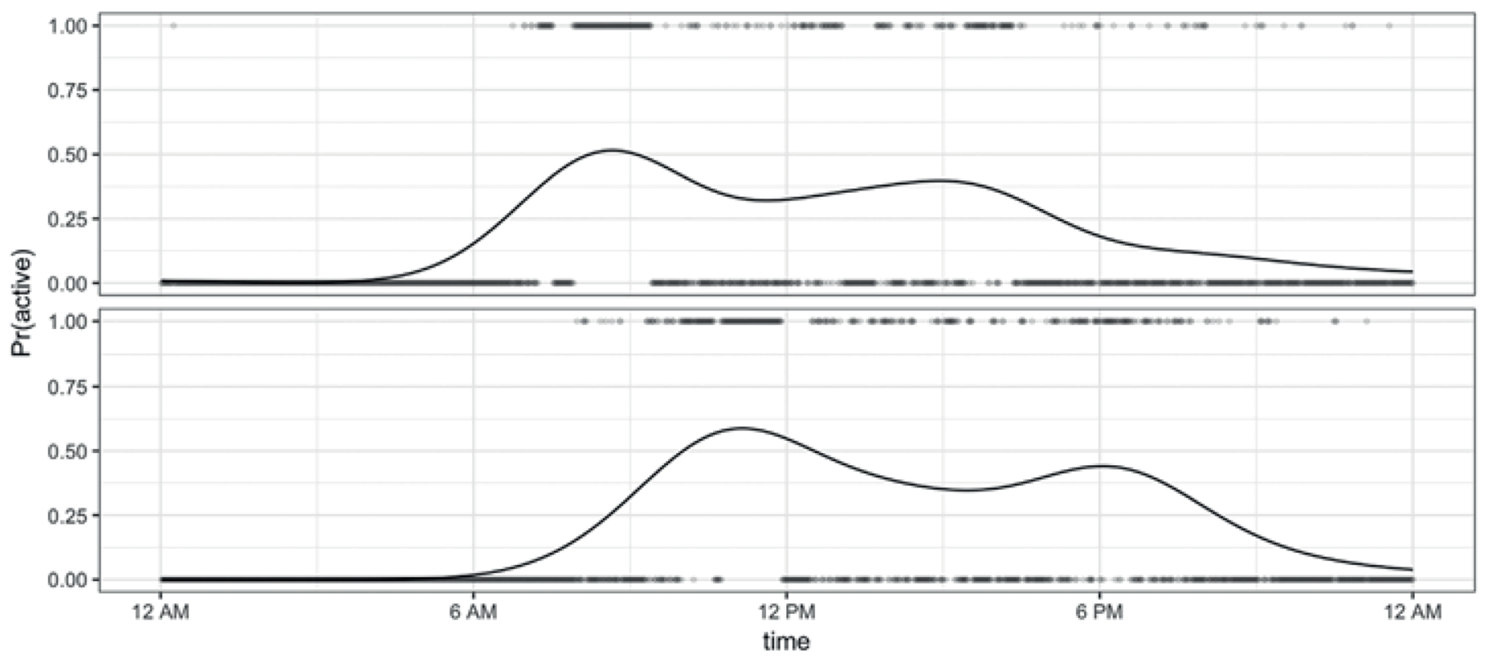
Points are binary curves for two subjects from the BLSA data before registration, where values of 1 and 0 represent activity and inactivity, respectively. The solid curves are estimates of the latent probability of activity, ${\mu }_i(t)$, and are fit for each subject using kernel smoothers.

Functional data often include both phase displacement, the misalignment of major features shared across curves, and amplitude variability. The process underlying phase variation may itself be of interest; additionally, when the interest is primarily in the amplitude variation, phase variation can artificially distort analyses of amplitude and mask the shared data structure. Methods for curve registration, which transform functional data to align features, are focused on addressing the problem of phase variation. The goal of registration is to warp the functional domain, which we will refer to as time, so that phase variation is minimized and the major features of the curves are aligned. This process necessitates a distinction between chronological time $\left(t_i^{\mathrm{*}}\right)$, which is the originally observed time for each subject, and internal time (t), which is the unobserved time on which major features are aligned across subjects (chronological and internal time are often referred to in the functional data literature as clock and system time, respectively). Stated differently, internal time is the true but unknown time over which aligned curves are generated and chronological time is the shifted time on which misaligned curves are observed. The registration problem amounts to recovering the subject-specific warping functions $h_i:t\mapsto t_i^{\mathrm{*}}$ which map internal time to chronological time. Inverse warping functions $h_i^{-1}\left(t_i^{\mathrm{*}}\right)$ can then be used to obtain aligned curves $Y_i(t)$ from observed data $Y_i\left(t_i^{\mathrm{*}}\right)$. To emphasize the conceptual difference between chronological and internal times, we index $t_i^{\mathrm{*}}$ by subject but do not index t.

We are interested in registering actigraphy data that comes from the Baltimore Longitudinal Study of Aging. The BLSA is an observational study of healthy aging and included an accelerometer for monitoring activity (Schrack et al., 2014). Our dataset includes 592 people, for whom accelerometer observations are gathered over 24 hours in one-minute epochs giving chronological times on equally spaced grids of length 1440. We are especially interested in activity and inactivity, defined using a threshold of raw accelerometer observations, as both low activity levels and excessive sedentary behavior have been associated with poor health outcomes. Moreover, there is a growing research interest in understanding temporal/diurnal patterns of accumulation of sedentary time (Martin et al., 2014; Diaz et al., 2017). However, those analyses typically report diurnal averages that ignore the differences between subject specific wake time and mix together amplitude and phase.

The left panel of Figure 2 shows observed binary curves against chronological time. In this plot subjects appear in rows, with active and inactive minutes shown in dark and light shades, respectively. This figure clearly shows the variability in the timing of inactivity across subjects, who may start or end the day at different times, and may accrue inactive minutes in sedentary bouts at different times. Such misalignment attenuates the diurnal patterns of activity that we believe to be present based on the naturally occurring circadian rhythm. The right panel of Figure 2 shows estimates of the unregistered mean ${\mu }_i\left(t_i^{\mathrm{*}}\right)$ obtained using a Gaussian kernel smoother; these smooths illustrate the phase misalignment across subjects. The shift in timing of activity and inactivity is also seen in Figure 1. Specifically, the subject in the top row wakes up early, has a peak of activity, and then has a low activity level for the rest of the day, while the subject below has a similar but shifted pattern of behavior.

Figure 2.

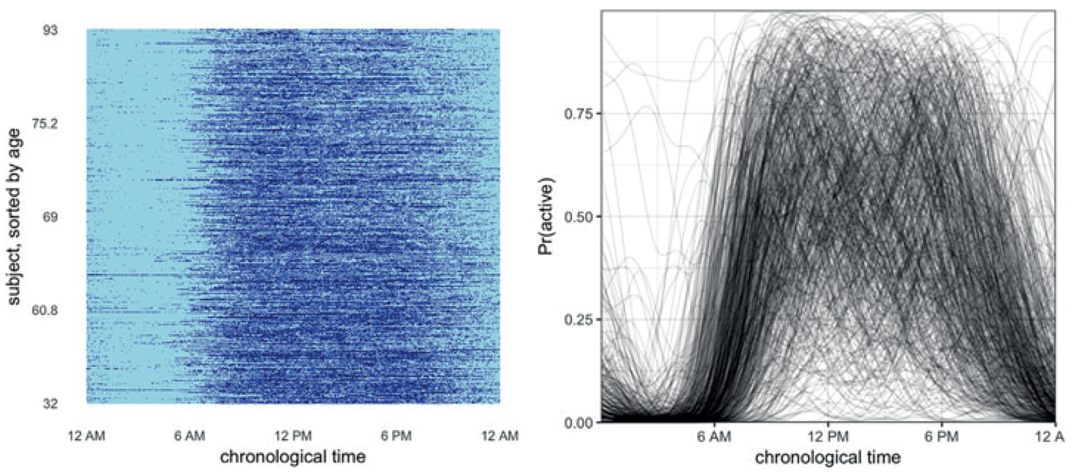
Plots of the unregistered data for 592 subjects at all 1440 minutes observed. At left is a lasagna plot, where row is the binary curve for a single subject and inactive and active observations are colored in light and dark shades, respectively. The rows are sorted by age, so that youngest subjects are at the bottom of the plot and oldest subjects are at the top. At right are smoothed curves for each subject, fit using kernel smoothers. This figure appears in color in the electronic version of this article.

We propose novel methods for the registration of exponential family functional data, with emphasis on binary curves. Due to data size computational efficiency is critical, and we take this into consideration at each step of our method development. Section 2 provides a review of relevant literature on registration and exponential-family functional principal components analysis; Section 3 details our methods; Section 4 shows simulation results, and Section 5 applies our method to the BLSA data. We conclude with a discussion in Section 6.

2. Literature Review

Our method draws on two distinct bodies of work in functional data analysis, which we review below. First, in 2.1, we review curve registration; this literature is primarily focused on Gaussian curves, with relatively little existing work for non-Gaussian curves. Then, in 2.2, we give an overview of exponential family FPCA, which is itself a relatively new area of interest in functional data analysis.

2.1. Registration

Several approaches for registering functional data have been proposed; we review these briefly, and suggest Marron et al. (2015) for a more detailed overview. Early approaches include dynamic time warping and landmark registration; for some time, however, template registration methods have been preferred. Template registration aligns each curve to a template curve by optimizing an objective function. This approach necessitates choosing the template, the objective function, and the optimization approach.

A common approach to template registration uses functional principal component analysis (FPCA) to select the template (Kneip and Ramsay, 2008). First these methods estimate the template, and then estimate the warping functions for a given template; these steps are iterated until convergence. Warping functions are estimated using a sum of squared errors approach, often penalized to enforce smoothness. There is a large registration literature operating under and expanding this framework, including Sangalli et al. (2010) and Hadjipantelis et al. (2015). Intuitively, functional principal components describe the main directions of variation in a set of curves, making FPCA a natural tool for identifying the features to which data is registered.

Srivastava et al. (2011) introduce a metric for calculating warping functions based on the Fisher–Rao distance. They calculate a Karcher mean template and define a square root slope function transform (SRSF) of the observed curves. Minimizing the ${𝕃}^2$ norm between two SRSFs is equivalent to minimizing their Fisher–Rao distance. Since the SRSF uses the derivative of the observed curve, the data to be registered are required to be smooth. The Fisher–Rao metric has been the basis for several recent approaches to registration, some which compute parameter values using dynamic programming (Srivastava et al., 2011; Wu and Srivastava, 2014), and others which use Riemannian optimization (Huang et al., 2014). Many of the SRSF-based approaches are implemented in the fdasrvf package (Tucker, 2017).

Although most work in registration has focused on continuous data, there are two recent exceptions. Wu and Srivastava (2014) apply the SRSF approach to binary functional data by pre-smoothing data with a Gaussian kernel and registering the resulting smooth curves. Panaretos and Zemel (2016) present a theoretical framework for separation of amplitude and phase variation of random point processes. The authors formalize a set of regularity conditions for warping functions that includes smoothness, proximity to the identity map, and unbiasedness, and establish a set of nonparametric estimators. However, since these estimators register the unobserved probabilities of the point processes, the authors also begin by smoothing binary curves using kernel density estimation.

In contrast to previous literature on registration, we develop an approach that can be applied to continuous and discrete data and does not require presmoothing. We also emphasize computational efficiency, an important matter given our high-dimensional data application.

2.2. FPCA for Exponential Family Curves

Functional principal components analysis is popular for identifying modes of variation in functional data. The most common approaches to FPCA decompose the variance-covariance matrix of demeaned functional observations; see Yao et al. (2005) or Goldsmith et al. (2013) for details on this approach. Hall et al. (2008) adapted the methods in Yao et al. (2005) for binary functional data by positing a smooth latent Gaussian process and then estimating and decomposing the covariance of this process. Serban et al. (2013) refined and extended this approach by improving approximations in the estimation procedure, increasing accuracy for rare events, and allowing spatial structures. However, as demonstrated in Gertheiss et al. (2017), the adaptation of Yao et al. (2005) to exponential family data has an inherent bias due to reliance on a marginal rather than conditional mean estimate.

Probabilistic FPCA is an appealing alternative to the covariance smoothing approach. This framework conceptualizes PCA as a likelihood-based model, can be approached from a Bayesian perspective, and easily accounts for sparse or irregular data. Tipping and Bishop (1999) introduce probabilistic PCA, and a related approach is used by James et al. (2000) for functional data. van der Linde (2008) extends probabilistic FPCA to binary and count data through a Taylor-approximated likelihood function, while Goldsmith et al. (2015) uses a fully Bayesian parameter specification for generalized FPCA and function-on-scalar regression. Because these approaches often relate the expected value of observed data to a smooth latent process through a link function, they are referred to as methods for generalized FPCA or GFPCA. Because all parameters are estimated simultaneously rather than sequentially, the probabilistic framework avoids the bias inherent in the covariance decomposition approach.

Our contributions to this literature focus on improving accuracy and efficiency for binary FPCA by estimating parameters in a probabilistic framework using a novel variational EM algorithm. To do this, we adapt the approach developed by Jaakkola and Jordan (1997) for logistic regression, which has since been extended to (non-functional) binary PCA (Tipping, 1999) and multi-level PCA (Yue, 2016). These methods rely on a variational approximation to the Bernoulli likelihood that is a true lower bound and allows for closed form updates of parameters. In contrast to van der Linde (2008), which uses a second-order Taylor expansion of the log likelihood to approximate a lower bound to the true distribution, our variational approximation is a true lower bound. While our method is optimized for binary data, similar derivations are possible for functional data from other exponential family distributions.

Consistent with this literature modeling exponential family curves, we assume a latent Gaussian process (LGP) generative model for our exponential family functional data. The LGP model assumes an unobserved smooth mean curve that serves as a “functional” natural parameter for the corresponding exponential family and from which the observed exponential family functional data is stochastically generated. In the case of binary data, the latent process is an unobserved smooth probability curve.

3. Methods

We first introduce the conceptual framework for our approach. Our goal is to estimate inverse warping functions $h_i^{-1}$ which map unregistered chronological time $t_i^{\mathrm{*}}$ to registered internal time t such that $h_i^{-1}\left(t_i^{\mathrm{*}}\right)=t$. Then for subject i, the unregistered and registered response curves are $Y_i\left(t_i^{\mathrm{*}}\right)$ and $Y_i(t)=Y_i\left\{h_i^{-1}\left(t_i^{\mathrm{*}}\right)\right\}$, respectively. Without loss of generality, we assume both $t^{\mathrm{*}}$ and t are on [0, 1]. We require that functions $h_i^{-1}$ are monotonically increasing and satisfy the endpoint constraints $h_i^{-1}(0)=0$ and $h_i^{-1}(1)=1$. Notationally, we combine warping functions with exponential family GFPCA through the following:

$$\begin{gathered} E\left[Y_i\left\{h_i^{-1}(t_i^{\text{*}})\right\}\mid c_i,h_i^{-1}\right]={\mu }_i(t) \\ g\left\{{\mu }_i(t)\right\}=\alpha (t)+\sum _{k=1}^K{c}_{ik}{\psi }_k(t). \end{gathered}$$ (1)

The aligned response curves $Y_i\left\{h_i^{-1}\left(t_i^{\mathrm{*}}\right)\right\}$ for each $t_i^{\mathrm{*}}\in [\mathrm{0,1}]$ arise from the canonical exponential family of distributions with density

$$P\left[Y_i\left\{h_i^{-1}(t_i^{\text{*}})\right\}\mid {\mu }_i(t)\right]=\text{exp}\{(Y_i\{h_i^{-1}(t_i^{\text{*}})\}g\{{\mu }_i(t)\}-b[g\{{\mu }_i(t)\}])/\phi +c[Y_i\{h_i^{-1}(t_i^{\text{*}})\},\phi ]\}$$ (2)

where $E\left[Y_i\left\{h_i^{-1}\left(t_i^{\mathrm{*}}\right)\right\}\mid {\mu }_i(t)\right]={\mu }_i(t)=b^{\prime }\left[g\left\{{\mu }_i(t)\right\}\right],Var\left[Y_i\left\{h_i^{-1}\left(t_i^{\mathrm{*}}\right)\}\right.\right.\left.\mid {\mu }_i(t)\right]=b^{″}\left[g\left\{{\mu }_i(t)\right\}\right]\phi$, and $\phi$ is the dispersion parameter. The subject-specific means ${\mu }_i(t)$ implicitly condition on parameters in model (1) and are used as templates in our warping step. Through link function $g$, the ${\mu }_i(t)$ are related to a linear predictor containing the population level mean $\alpha (t)$ and a linear combination of population level basis functions $\psi (t)$ and subject-specific score vectors ${\mathit{c}}_i\sim N\left(0,{\mathit{I}}_{K\times K}\right)$. This formulation assumes that registered curves can be decomposed using GFPCA and, in doing so, places both registration and GFPCA in a single model.

Our estimation method is based on model (1) and alternates between the following steps:

1. Subject-specific means ${\mu }_i(t)$ are estimated via probabilistic GFPCA, conditional on the current estimate of inverse warping functions $h_i^{-1}\left(t_i^{\mathrm{*}}\right)$.

2. Inverse warping functions $h_i^{-1}$ are estimated by maximizing the log likelihood of the exponential family distribution under monotonicity and endpoint constraints on $h_i$, conditional on the current estimate of ${\mu }_i$.

We iterate between steps (1) and (2) until curves are aligned.

Similar registration approaches for continuous-valued response curves have used the squared error loss for optimizing warping functions which, in a Gaussian setting, is equivalent to maximizing the likelihood function. However, our likelihood-based approach, which registers non-Gaussian data by extending the exponential-family framework, is novel. In contrast to registration methods for discrete functional data, we register observed binary curves using smooth templates rather than aligning pre-smoothed functional data. Because our application has 592 subjects measured at 1440 time points each, computational efficiency is critical. To this end, we develop a novel fast approach to binary FPCA in Step 1, which we describe in Section 3.1, and optimize speed in estimating warping functions in Step 2, which we describe in Section 3.2.

3.1. Binary FPCA

We first detail our novel EM approach to binary FPCA. Model (1) provides a conceptual framework, assuming that each curve $Y_i(t)$ is evaluated over internal time $t\in [\mathrm{0,1}]$. In practice, data for subject $i$ is observed on the discrete grid, ${\mathit{t}}_i=\left\{t_{i1},\dots ,t_{i{D}_i}\right\}$, which may be irregular across subjects, and therefore (in contrast to $t$) is indexed by subject. Functions indexed by the vector ${\mathit{t}}_i$ are $D_i\times 1$ vectors of those functions evaluated on the observed time points (e.g., ${\mathit{Y}}_i\left({\mathit{t}}_i\right)={\left\{Y_i\left(t_{i1}\right),\dots ,Y_i\left(t_{i{D}_i}\right)\right\}}^T$ and $\left.{\psi }_k\left({\mathit{t}}_i\right)={\left\{{\psi }_k\left(t_{i1}\right),\dots ,{\psi }_k\left(t_{i{D}_i}\right)\right\}}^T\right)$. The population level mean $\alpha (t)$ and principal components ${\psi }_k(t)$, $1\le k\le K$, are expanded using a fixed B-spline basis, ${\mathbf{\Theta }}_{\varphi }(t)$, of $K_{\varphi }$ basis functions ${\theta }_1(t),\dots ,{\theta }_{K_{\varphi }}(t)$. Let ${\mathbf{\Theta }}_{\varphi }\left({\mathit{t}}_i\right)$ be the $D_i\times K_{\varphi }$ B-spline matrix evaluated at ${\mathit{t}}_i$ and a $1\times K_{\varphi }$ vector when evaluated at a single point $t_{ij}$; then $\alpha \left({\mathit{t}}_i\right)={\mathbf{\Theta }}_{\varphi }\left({\mathit{t}}_i\right){\mathit{\alpha }}_{\mathrm{\Theta }}$ and $\mathrm{\Psi }\left({\mathit{t}}_i\right)=\left\{{\psi }_1\left({\mathit{t}}_i\right),\dots ,{\psi }_K\left({\mathit{t}}_i\right)\right\}={\mathbf{\Theta }}_{\varphi }\left({\mathit{t}}_i\right){\mathbf{\Psi }}_{\mathrm{\Theta }}$ where the vector ${\mathit{\alpha }}_{\mathrm{\Theta }}$ and matrix ${\mathbf{\Psi }}_{\mathrm{\Theta }}$ of size $K_{\varphi }\times K$ contain the spline coefficients for the mean and principal components, respectively. Observed on the discrete grid ${\mathit{t}}_i$, the linear predictor in (1) becomes

$$g\{{\mu }_i({\mathit{t}}_i)\}={\Theta }_{\varphi }(t_i)({\mathit{\alpha }}_{\text{Θ}}+{\Psi }_{\text{Θ}}{\mathit{c}}_i).$$ (3)

We estimate parameters in model (3) using an EM algorithm that incorporates a variational approximation. We assume ${\mathit{c}}_i\sim \mathit{MVN}(0,I)$. For the binary case that is our main interest, $g(\cdot )$ is the logit function, for each point on the grid for the ith subject, $Y_i\left(t_{ij}\right)\sim \mathit{Bernoulli}\left\{{\mu }_i\left(t_{ij}\right)\right\}$ where ${\mu }_i\left(t_{ij}\right)=P\left\{Y_i\left(t_{ij}\right)=1\mid {\mathit{c}}_i\right\}$. It is convenient to rewrite the probability density function as

$$P\left\{Y_i(t_{ij})\mid {\mathit{c}}_i\right\}=g^{-1}\left[\{2Y_i(t_{ij})-1\}\{{\Theta }_{\varphi }(t_{ij})({\mathit{\alpha }}_{\text{Θ}}+{\Psi }_{\text{Θ}}{\mathit{c}}_i)\}\right],$$ (4)

so that the full unobserved joint likelihood for the observations and score vectors is

$$\begin{gathered} L(\mathit{Y},\mathit{c})\propto \prod _{i=1}^I\prod _{j=1}^{D_i}{g}^{-1}\left[\{2Y_i(t_{ij})-1\}\{{\Theta }_{\varphi }(t_{ij})({\mathit{\alpha }}_{\text{Θ}}+{\Psi }_{\text{Θ}}{\mathit{c}}_i)\}\right] \\ \times \prod _{i=1}^I\text{exp}\left(-\frac{{\mathit{c}}_i^T{\mathit{c}}_i}{2}\right). \end{gathered}$$ (5)

Let scalar $A_i\left(t_{ij}\right)={\mathbf{\Theta }}_{\varphi }\left(t_{ij}\right)\left({\mathit{\alpha }}_{\mathrm{\Theta }}+{\mathbf{\Psi }}_{\mathrm{\Theta }}{\mathit{c}}_i\right)$ and $\lambda (z)=\frac{0.5-g^{-1}(z)}{2z}$. A variational approximation to (4), based on the approximation in Jaakkola and Jordan (1997), is

$$\begin{gathered} \tilde{P}\{Y_i(t_{ij})\mid {\mathit{c}}_i,{\xi }_i(t_{ij})\}=g^{-1}\{{\xi }_i(t_{ij})\}\text{exp}[\frac{\left\{2Y_i(t_{ij})-1\right\}{A}_i(t_{ij})-{\xi }_i(t_{ij})}{2} \\ +\lambda \left\{{\xi }_i(t_{ij})\right\}\left\{A_i{(t_{ij})}^2-{\xi }_i{(t_{ij})}^2\right\}] \end{gathered}$$ (6)

and is further discussed in Web Appendix A. The resulting variational joint likelihood is

$$\tilde{L}(\mathit{Y},\mathit{c})\propto \prod _{i=1}^I\prod _{j=1}^{D_i}\tilde{P}\left\{Y_i(t_{ij})\mid {\mathit{c}}_i,{\xi }_i(t_{ij})\right\}\times \prod _{i=1}^I\text{exp}\left(-\frac{{\mathit{c}}_i^T{\mathit{c}}_i}{2}\right).$$ (7)

We use an EM algorithm to obtain parameter estimates from (7) by (i) finding the posterior distribution of the scores; (ii) maximizing $\tilde{L}(\mathit{Y},\mathit{c})$ with respect to $\mathit{\xi }$; and (iii) maximizing the variational likelihood with respect to ${\mathit{\alpha }}_{\mathrm{\Theta }}$ and ${\mathbf{\Psi }}_{\mathrm{\Theta }}$. These three steps are described in Sections 3.1.1, 3.1.2, and 3.1.3; more details and simulations comparing to other GFPCA methods are given in the Appendix. A solution is attained when the squared difference between parameter estimates and their previous solution become arbitrarily small.

3.1.1. Calculating posterior scores.

The posterior scores for each subject, derived via Bayes’ rule, follow a multivariate normal distribution ${\mathit{c}}_i\mid Y_i\left({\mathit{t}}_i\right),{\xi }_i\left({\mathit{t}}_i\right)\sim \mathrm{MVN}\left({\mathit{m}}_i,{\mathit{C}}_i\right)$ with:

$${\mathit{C}}_i={\left({\mathit{I}}_{K\times K}-2{\Psi }_{\text{Θ}}^T{\Theta }_{\varphi }{({\mathit{t}}_i)}^T\mathit{diag}[\lambda \{{\xi }_i({\mathit{t}}_i)\}]{\Theta }_{\varphi }({\mathit{t}}_i){\Psi }_{\text{Θ}}\right)}^{-1}$$

and

$$\begin{gathered} {\mathit{m}}_i={\mathit{C}}_i({\Psi }_{\text{Θ}}^T{\Theta }_{\varphi }{({\mathit{t}}_i)}^T\{Y_i(t_i)-\frac{1}{2}\} \\ +2{\Psi }_{\text{Θ}}^T{\Theta }_{\varphi }{({\mathit{t}}_i)}^T\mathit{diag}[\lambda \{{\xi }_i({\mathit{t}}_i)\}]{\Theta }_{\varphi }({\mathit{t}}_i){\mathit{\alpha }}_{\text{Θ}}) \end{gathered}$$

where ${\xi }_i\left({\mathit{t}}_i\right)$ is a vector of length $D_i$ and $\mathit{diag}\left[\lambda \left\{{\xi }_i\left({\mathit{t}}_i\right)\right\}\right]$ is a $D_i\times D_i$ diagonal matrix.

3.1.2. Maximizing $\tilde{\mathit{L}}(\mathit{Y},\mathit{c})$ with respect to $\mathit{\xi }$.

We maximize the variational likelihood with respect to ${\xi }_i^2$, obtaining

$$\begin{gathered} {\widehat{\xi }}_i{(t_{ij})}^2=E_{{\tilde{P}}_{post}}\left\{A_i{(t_{ij})}^2\right\} \\ ={\mathit{\alpha }}_{\text{Θ}}^T{\Theta }_{\varphi }{(t_{ij})}^T{\Theta }_{\varphi }(t_{ij}){\mathit{\alpha }}_{\text{Θ}}+2{\mathit{\alpha }}_{\text{Θ}}^T{\Theta }_{\varphi }{(t_{ij})}^T{\Theta }_{\varphi }(t_{ij}){\Psi }_{\text{Θ}}{\mathit{m}}_i \\ +\text{tr}\left\{{\Psi }_{\text{Θ}}^T{\Theta }_{\varphi }{(t_{ij})}^T{\Theta }_{\varphi }(t_{ij}){\Psi }_{\text{Θ}}{\mathit{C}}_i\right\}+{\mathit{m}}_i^T{\Psi }_{\text{Θ}}^T{\Theta }_{\varphi }{(t_{ij})}^T{\Theta }_{\varphi }(t_{ij}){\Psi }_{\text{Θ}}{\mathit{m}}_i \end{gathered}$$

where the expectation is taken with respect to the posterior distribution $\tilde{P}\left\{{\mathit{c}}_i\mid Y_i\left({\mathit{t}}_i\right),{\xi }_i\left({\mathit{t}}_i\right)\right\}$, using estimates of ${\mathit{\alpha }}_{\mathrm{\Theta }}$ and ${\mathbf{\Psi }}_{\mathrm{\Theta }}$ from the previous iteration.

3.1.3. Maximizing $\tilde{\mathit{L}}(\mathit{Y},\mathit{c})$ with respect to ${\mathit{\alpha }}_{\Theta }$ and ${\mathit{\Psi }}_{\Theta }$.

In this step, we jointly estimate vectors of spline coefficients, which distinguishes our approach from previous binary PCA techniques and which entails additional complexity in the derivation of updates. The introduction of the spline basis and associated coefficients lowers the dimensionality of the estimation problem and enforces smoothness of the resulting ${\widehat{\mu }}_i(t)$.

In order to obtain updates for our population-level basis coefficients, we introduce a new representation of the model which is mathematically equivalent to the parameterization in model (4) and easier to maximize. Let ${\mathit{s}}_i={\left({\mathit{c}}_i^T,1\right)}^T$ of dimension $(K+1)\times 1$ and $\mathbf{\Phi }={\left({\mathbf{\Psi }}_{\mathrm{\Theta }}^T,{\mathit{\alpha }}_{\mathrm{\Theta }}\right)}^T$ of dimension $(K+1)\times K_{\varphi }$, and $vec(\mathbf{\Phi })$ be a vectorized version of $\mathbf{\Phi }$ with dimension $K_{\varphi }(K+1)\times 1$. We can rewrite $A_i\left({\mathit{t}}_i\right)$ as $A_i\left({\mathit{t}}_i\right)={\mathbf{\Theta }}_{\varphi }\left({\mathit{t}}_i\right)\left({\mathit{\alpha }}_{\mathrm{\Theta }}+{\mathbf{\Psi }}_{\mathrm{\Theta }}{\mathit{c}}_i\right)=\left\{{\mathbf{\Theta }}_{\varphi }\left({\mathit{t}}_i\right)\otimes {\mathit{s}}_i^T\right\}vec(\mathbf{\Phi })$, where $\otimes$ is the Kronecker product. Maximizing the variational log-likelihood in this reparameterized form gives updates

$$\begin{gathered} \mathit{vec}(\widehat{\Phi })={-(\sum _{i}2{\Theta }_{\varphi }{({\mathit{t}}_i)}^T\mathit{diag}[\lambda \{{\xi }_i({\mathit{t}}_i)\}]{\Theta }_{\varphi }({\mathit{t}}_i)\otimes \widehat{{\mathit{s}}_i{\mathit{s}}_i^T}))}^{-1} \\ \left[\sum _i{\left\{Y_i({\mathit{t}}_i)-\frac{1}{2}\right\}}^T\{{\Theta }_{\varphi }({\mathit{t}}_i)\otimes {\widehat{\mathit{s}}}_i^T\}\right] \end{gathered}$$

where $\widehat{{\mathit{s}}_i}={\left({\mathit{m}}_i^T,1\right)}^T$ and $\widehat{{\mathit{s}}_i{\mathit{s}}_i^T}=\left(\begin{array}{cc}& {\mathit{C}}_i+{\mathit{m}}_i{\mathit{m}}_i^T{\mathit{m}}_i\\ {\mathit{m}}_i^T& 1\end{array}\right)$. The first $K$ rows of $\widehat{\mathit{vec}\mathbf{\Phi }}$ are the K columns of ${\widehat{\mathbf{\Psi }}}_{\mathrm{\Theta }}$, and the last $K_{\varphi }$ rows are ${\widehat{\mathit{\mu }}}_{\mathrm{\Theta }}$.

3.2. Binary Registration

We now turn to the second step in our iterative algorithm, in which warping functions are estimated for each subject conditionally on the target function ${\mu }_i(t)$. Conceptually, our approach is to maximize the exponential family likelihood function given by integrating the density in equation (2) over time. We maximize with respect to the inverse warping function $h_i^{-1}\left(t_i^{\mathrm{*}}\right)$, subject to the constraint that $h_i^{-1}\left(t_i^{\mathrm{*}}\right)$ is monotonic with endpoints fixed at the minimum and maximum of our domain. For binary data we maximize the Bernoulli log-likelihood

$$\begin{gathered} l(h_i^{-1};Y_i,{\mu }_i)=\int (Y_i(t_i^{\text{*}})\text{log}{\mu }_i\{h_i^{-1}(t_i^{\text{*}})\}+\{1-Y_i(t_i^{\text{*}})\} \\ \text{log}[1-{\mu }_i\{h_i^{-1}(t_i^{\text{*}})\}]). \end{gathered}$$ (8)

Again, functions are observed on a discrete grid in practice, and we differentiate between subject-specific finite grids for chronological time ${\mathit{t}}_i^{\mathrm{*}}=\left\{t_{i1}^{\mathrm{*}},\dots ,t_{i{D}_i}^{\mathrm{*}}\right\}$ and internal time ${\mathit{t}}_i=\left\{t_{i1},\dots ,t_{i{D}_i}\right\}$. Using notation similar to Section 3.1, we let $Y_i\left({\mathit{t}}_i^{\mathrm{*}}\right),Y_i\left({\mathit{t}}_i\right)$, and $h_i^{-1}\left({\mathit{t}}_i^{\mathrm{*}}\right)$ be $D_i\times 1$ vectors corresponding to observed responses, registered responses, and inverse warping functions, respectively. We expand $h_i^{-1}\left({\mathit{t}}_i^{\mathrm{*}}\right)$ using a B-spline basis, ${\mathbf{\Theta }}_h\left({\mathit{t}}_i^{\mathrm{*}}\right)$, of dimension $D_i\times K_h$ to take the form $h_i^{-1}\left({\mathit{t}}_i^{\mathrm{*}}\right)={\mathbf{\Theta }}_h\left({\mathit{t}}_i^{\mathrm{*}}\right){\mathit{\beta }}_i={\mathit{t}}_i$. The $K_h\times 1$ vector of spline coefficients ${\mathit{\beta }}_i$ allows us to express $h_i^{-1}\left({\mathit{t}}_i^{\mathrm{*}}\right)$, and is the target of our estimation problem. We estimate ${\mathit{\beta }}_i$ separately for each subject using constrained optimization and loop over subjects.

We modify the conceptual likelihood in equation (8) to incorporate the spline basis expansion of $h^{-1}$ and to express data over the observed finite grid, which yields

$$\begin{gathered} l\{{\mathit{\beta }}_i;Y_i({\mathit{t}}_i^{\text{*}}),{\mu }_i(\cdot )\}\propto \sum _{j=1}^{D_i}(Y_i(t_{ij}^{\text{*}})\text{log}{\mu }_i\{{\Theta }_h(t_{ij}^{\text{*}}){\mathit{\beta }}_i\} \\ +\{1-Y_i(t_{ij}^{\text{*}})\}\text{log}\left[1-{\mu }_i\{{\Theta }_h(t_{ij}^{\text{*}}){\mathit{\beta }}_i\}\right]). \end{gathered}$$ (9)

Recall that ${\mu }_i(\cdot )$ from (3) is the subject-specific mean found in the FPCA step. Estimates are constrained to be monotonic with fixed endpoints. The constraints ensure that our resulting estimates for t are monotonic and span the desired domain. We implement these constraints using linear constraint matrices, which we provide in Appendix A. The constrained optimization can be made more efficient with an analytic form of the gradient. The gradient for the general exponential family case and for the Bernoulli loss in particular also appear in Appendix A.

3.3. Implementation

Our methods are implemented in R and are publicly available on GitHub as part of the registr package (Wrobel, 2018). For Step 1, binary FPCA is custom-written with a C++ backend for estimation. For Step 2, we implement linearly constrained optimization with the constrOptim() function, which uses an adaptive barrier algorithm to minimize an objective function subject to linear inequality constraints. If an analytic gradient of the objective function is not provided, then Nelder–Mead optimization is used, otherwise BFGS, a gradient descent algorithm, is used. By implementing an analytic gradient we improve accuracy and computational efficiency of our estimation.

Though our simulated and real data examples are observed on a dense regular grid, the registr package handles both sparse and irregular functional data. For visualizing results, registr is compatible with refund.shiny, an R package that produces interactive graphics for functional data analyses (Wrobel et al., 2016).

4. Simulations

We assess the accuracy and computational efficiency of our method using data simulated to mimic our motivating study, and compare to competing approaches described below.

4.1. Simulation Design

Binary functions in simulated datasets are designed to exhibit a circadian rhythm, so that simulated participants are more likely to be inactive at the beginning and end of the domain (“day”) and more likely to be active in the middle of the day. Overall activity levels vary across simulated participants, as do the timing of the active period. Participants exhibit two main active periods separated by a dip, which is consistent with the BLSA data.

We first generate a grid of chronological times ${\mathit{t}}_i^{\mathrm{*}}$, which is equally spaced and shared across subjects. We generate inverse warping functions $h_i^{-1}\left({\mathit{t}}_i^{\mathrm{*}}\right)$ using a B-spline basis with 3 degrees of freedom; coefficients are chosen from a uniform(0,1) distribution and placed in increasing order to ensure monotonically increasing warping functions. The internal times ${\mathit{t}}_i$ for each subject are obtained by evaluating the inverse warping functions at ${\mathit{t}}_i^{\mathrm{*}}$. We simulate latent probability curves over internal time, ${\mu }_i\left({\mathit{t}}_i\right)$, from the model

$$\begin{gathered} E\left\{Y_i({\mathit{t}}_i)\mid c_i\right\}={\mu }_i({\mathit{t}}_i) \\ g\left\{{\mu }_i({\mathit{t}}_i)\right\}=\mathit{\alpha }({\mathit{t}}_i)+c_i\times \psi ({\mathit{t}}_i) \end{gathered}$$ (10)

where $\alpha \left({\mathit{t}}_i\right)$ and $\psi \left({\mathit{t}}_i\right)$ are constructed using a B-spline basis and $c_i\stackrel{i.i.d}{\sim }N(\mathrm{0,1})$. For each $t_{ij}\in i,j=1,\dots ,D_i$, binary observations $Y_i\left(t_{ij}\right)$ are sampled independently over $j$ from a Bernoulli distribution with $\mu \left(t_{ij}\right)$.

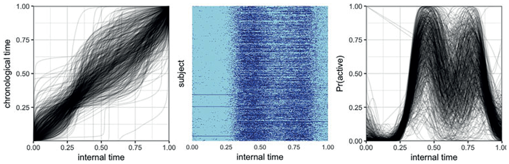
Unregistered data $Y_i\left({\mathit{t}}^{\mathrm{*}}\right)$, observed over the grid ${\mathit{t}}_i^{\mathrm{*}}$, are defined by the warping functions $h_i\left({\mathit{t}}_i\right)$. Figure 3 shows an example of a single simulated dataset, including latent probability curves on both ${\mathit{t}}_i^{\mathrm{*}}$ and $\mathit{t}$ (first row, first and second columns) and observed binary data (second row, first and second columns).

Figure 3.

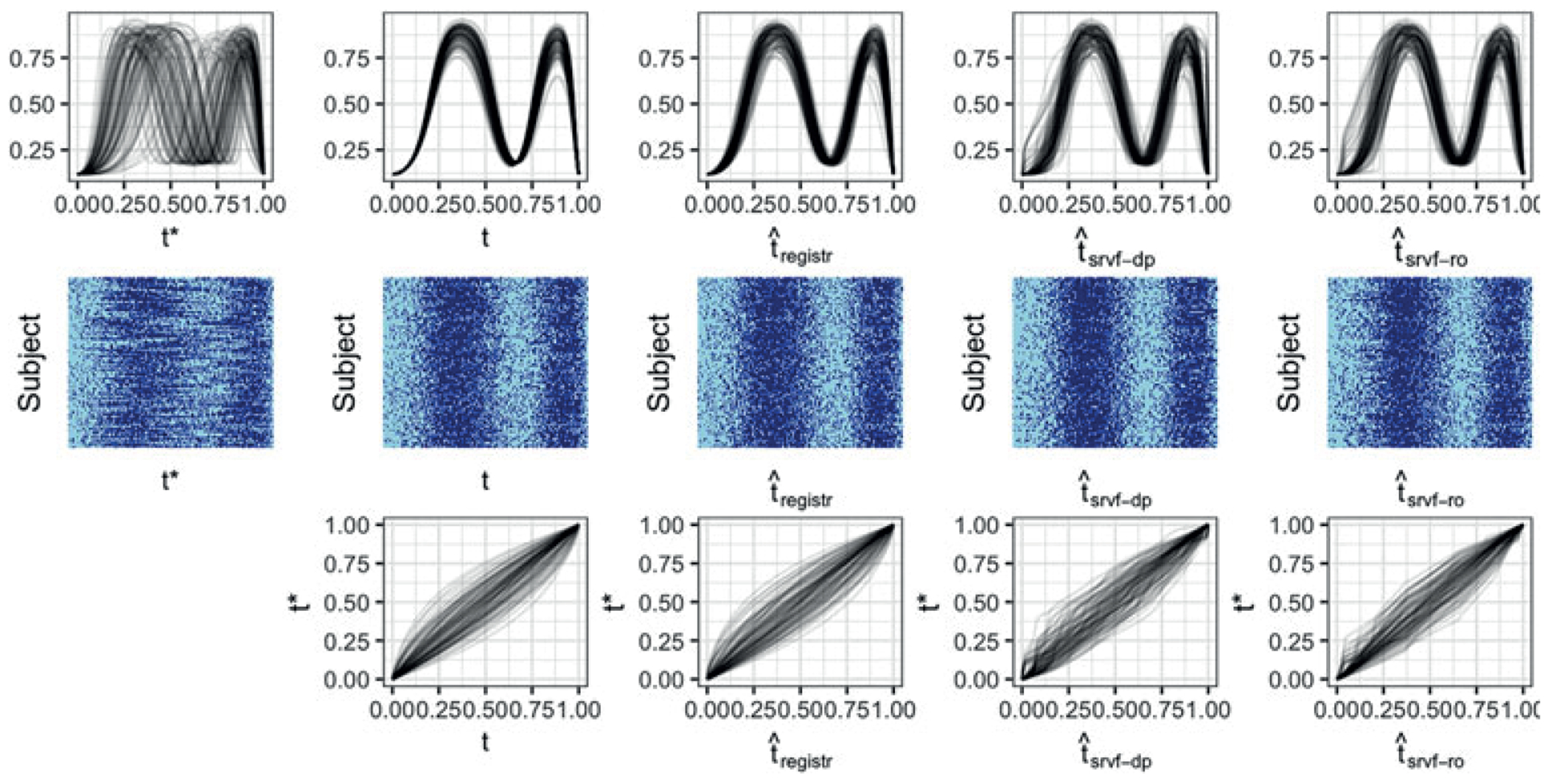
For top and center rows, from left to right we have: unregistered curves, curves registered using true inverse warping functions, curves registered using registr method, curves registered using fdasrvf method with dynamic programming optimization, curves registered using fdasrvf method with Riemannian optimization. The top row shows the true latent probability curves which are used to generate the binary curves but not used to estimate warping since they are unknown in a real data application. The middle row shows the binary curves as a heatmap-style plot, as in Figure 2. The bottom row shows the true, registr method, fdasrvf method with dynamic programming, and fdasrvf method with Riemannian optimization inverse warping functions. This figure appears in color in the electronic version of this article.

We evaluate the performance of our algorithm as a function of sample size and grid length. We simulate 25 datasets for each combination of sample sizes (50, 100, and 200) and grid lengths (taking values 100, 200, 400). For each dataset, we apply the methods in Section 3, denoted registr in text and figures below, setting $K_{\varphi }=9,K_h=3$, and using 1 FPC.

To provide a frame of reference, we compare our approach with two approaches based on the SRSF framework, both of which are implemented in the time_warping() function in the fdasrvf package (Tucker, 2017). Both implementations use smoothed versions of the binary data but use different optimization methods. The first uses dynamic programming, which is the default optimization choice for the fdasrvf software, and is denoted svrf-dp in text and figures below. The second uses Riemannian optimization and is denoted svrf-ro. For both competing approaches, observed binary data was smoothed using a box filter, which is built into the fdasrvf software. The number of box filter passes is a tuning parameter that must be selected, and we found that the overall registration results were sensitive to this choice. We considered several values (25, 50, 100, 200, and 400); in the following, we use 200 passes, which generally lead to better performance in our simulations.

Methods are compared in terms of estimation accuracy and computation time, with accuracy quantified using mean integrated squared error (MISE). For each subject, integrated squared error calculations are made comparing the estimated inverse warping functions for each method, ${\widehat{h}}_i^{-1}\left({\mathit{t}}_i^{\mathrm{*}}\right)$, to the true inverse warping functions $h_i^{-1}\left({\mathit{t}}_i^{\mathrm{*}}\right)$ such that $ISE={\int }_0^1{\left\{h_i^{-1}\left({\mathit{t}}_i^{\mathrm{*}}\right)-{\widehat{h}}_i^{-1}\left({\mathit{t}}_i^{\mathrm{*}}\right)\right\}}^{2}d{t}_i$. MISE is then the average of ISEs across subjects. A sensitivity analysis of our method’s performance across values of $K_{\varphi }$ and $K_h$ is given in the Appendix.

4.2. Simulation Results

Figure 3 shows a simulated dataset with 100 subjects observed over a grid with 200 time points. From left to right, columns show observed (unregistered) data; data observed on the true internal time t; and data aligned using the registr method, the srvf-dp method, and the srvf-ro method. The top row shows the latent mean curves, the middle row shows plots of observed binary data, and the bottom row shows inverse warping functions using true internal time t and estimated internal times ${\widehat{t}}_{\mathit{registr}},{\widehat{t}}_{svrf-dp}$, and ${\widehat{t}}_{\mathit{svrf-ro}}$. The latent probability curves illustrate the structure of the simulated data and the relative magnitudes of phase and amplitude variability. Binary curves illustrate the observed data, and include two periods of higher activity for each subject.

The results for registr in this example are encouraging, both for the latent curves and for the binary activity data in that phase variation is largely removed. Some amount of misalignment remains, which is attributable to the inherent sampling variability introduced when binary points are generated from the latent probabilities. The srvf-dp method also works reasonably well, although visual inspection of the probability curves and binary data suggests somewhat poorer alignment. The srvf-ro method has poorest alignment, although it also performs reasonably well and captures the major features in the data.

Figure 4 summarizes results across simulated datasets at different sample sizes and grid lengths; for reference, the data in Figure 3 has a median MISE for the registr method relative to other datasets generated with 100 subjects and 200 time points. The columns of Figure 4, from left to right, show results for datasets with 50, 100, and 200 subjects, respectively, and grid lengths of 100, 200, and 400 are shown within each panel. The top row shows box plots of MISE and the bottom row shows median computation times. Across all settings, registr outperforms both srvf-dp and srvf-ro methods in terms of the MISE; this is consistent with observations in Figure 3. With respect to computation time, although the methods are similar for small sample sizes and grid lengths, registr and srvf-ro scale as these increase, while the burden grows dramatically for srvf-dp.

Figure 4.

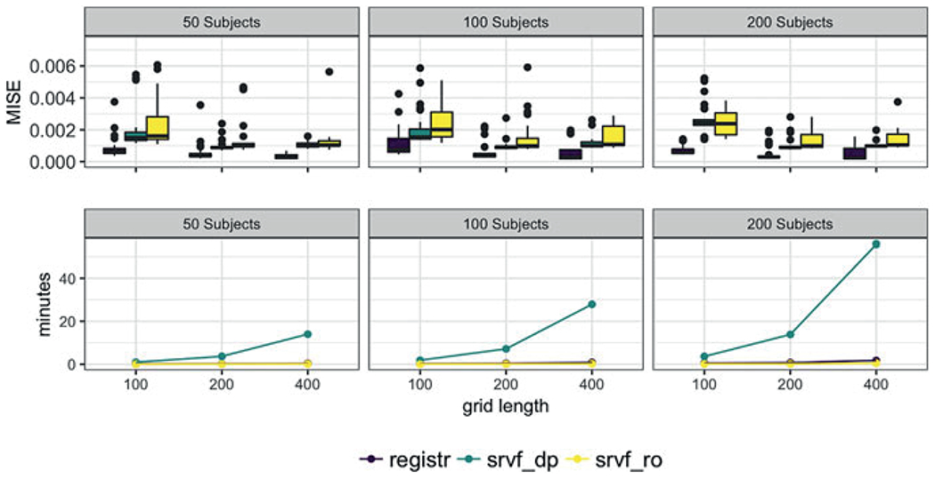
This figure shows mean integrated squared errors (top row) and median computation times (bottom row) for registr (darkest shade), srvf-dp (medium shade), and srvf-ro (lightest shade) methods across varying sample sizes and grid lengths. The columns, from left to right, show sample sizes 50, 100, and 200, respectively. Within each panel we compare grid lengths of 100, 200, and 400. This figure appears in color in the electronic version of this article.

5. Analysis

We now apply our method described in Section 3 to the BLSA data. These data contain 592 subjects with activity counts every minute over 24 hours, for a total of 1440 measurements per subject. BLSA participants wore the accelerometer for 5 days; we average across these days to establish a typical diurnal pattern for each participant, and then threshold the result at values of 10 counts per minute to obtain the binary activity curve to be registered. We fix the dimensions of the B-spline basis functions to $K_{\varphi }=8$ and $K_h=4$ and number of FPCs to $K=2$. Total computation time was 17 minutes. In the following, we discuss registered activity profiles using language that refers to times of day. However, it is important to remember throughout this section that registered curves are observed on internal time rather than chronological time, and times of day are person-specific in that sense.

Figure 5 shows the registered curves from the BLSA dataset, which can be compared with the observed data in Figure 2. After registration, there are two clear activity peaks: people tend to be active for an extended period of time after they wake up; this period is followed by a mid-day dip in activity, and a second, smaller, period of activity in the afternoon and evening. Figure 6 emphasizes this point, and the effect of registration, by plotting the subjects from Figure 1 after registration. The data for these two subjects are more closely aligned, as are the latent probabilities curves estimated from the aligned data. The left panel of Figure 5 shows the inverse warping functions which transform the BLSA data from the unregistered to the registered space.

Figure 5.

Plots of the registered BLSA data. Left panel shows inverse warping functions from alignment of the data; center panel shows a plot of the aligned binary data; and right panel shows smooths of the aligned data. See Figure 2 for the unregistered data. This figure appears in color in the electronic version of this article.

Figure 6.

These are binary curves for the same two subjects from the BLSA data as in Figure 1 but now the curves are registered. Here, the lines represent estimates of the latent probability that come from our binary FPCA algorithm.

The results of the applying the registration method to these data are consistent with expectations, in that the diurnal activity pattern observed across subjects after registration contains both morning and afternoon active periods and a period of relative inactivity around lunchtime. These results also emphasize the importance of assessing and removing phase variability in studies of daily activity patterns. The existence and number of “chronotypes,” or subjects who intrinsically prefer certain hours of the day (like the colloquial night owls or early birds), is the subject of intense debate in the circadian rhythm literature (Adan et al., 2012). Aligning observed activity data as a processing step may help inform this debate, and our results are consistent with the existence of distinct chronotypes in this population. The supplementary materials contain additional analysis results for the registration of data from each day of the week separately. These results are similar to those presented in this section.

6. Discussion

We present a novel approach to curve registration for functional data from exponential family distributions which avoids the need for pre-smoothing, and our attention to computational efficiency is necessitated by our data. Simulations suggest our approach compares favorably to competing methods in the settings we examined. Our scientific results are plausible and meaningful in the context of activity measurement. Finally, our code for registration and binary probabilistic FPCA is publicly available in the registr package.

Our approach assumes exponential family functional data is generated from a latent Gaussian process. While this is a common modeling choice for binary functional data that works well in practice, it may not provide a suitable framework for theoretical considerations in which the grid size goes to infinity. Possible future work building on Descary and Panaretos (2016), which considers modeling continuous functional data with both low rank structure and local correlation in the Gaussian setting, may provide a scientifically meaningful way forward but is beyond our current scope.

Though registr outperformed the SRSF-based approaches in our simulations, we expect that the SRSF method will be better suited to some cases including, potentially, smooth Gaussian curves. Indeed, when curves are absolutely continuous SRSF has the added theoretical benefits of translation and scale invariance and consistency of the warping procedure. For discrete data or noisy Gaussian data, where a smoothing parameter must be chosen before applying SRSF methods, it is unclear if any method will be uniformly superior and we recommend considering multiple approaches to registration.

Because of the nature of our application, we optimize performance for registering binary curves. While our method can be applied to functional data from any exponential family, one will not reap the computational benefits we highlight here without at least some additional work optimizing the FPCA algorithm for additional distributions; computationally efficient implementations for the Poisson distribution will be relevant for studies using accelerometer data. For our application, we chose to threshold activity count data and register the resulting binary curves, which aligned general patterns of activity and inactivity. Though we could have chosen to register the raw counts using a Poisson distribution, exploratory analyses suggested that aligning raw activity counts may be overly influenced by extreme values.

Though we focus on amplitude alignment for this article, the inverse warping functions contain information on phase variation and are potential analysis objects for future scientific work. Subsequent analyses will examine whether aligned data are more clearly affected by covariates like age and sex, and how the phase alignment relates to these covariates. Finally, we note that our emphasis has been on the temporal structure of inactivity, and additional work to connect these results with the accrual of sedentary minutes in bouts is needed.

References

- Adan A, Archer SN, Hidalgo MP, Di Milia L, Natale V, and Randler C (2012). Circadian typology: A comprehensive review. Chronobiology International 29, 1153–1175. [DOI] [PubMed] [Google Scholar]
- Descary M-H and Panaretos VM (2016). Functional data analysis by matrix completion. arXiv preprint arXiv:1609.00834. [Google Scholar]
- Diaz K, Howard V, Hutto B (2017). Patterns of sedentary behavior and mortality in u.s. middle-aged and older adults: A national cohort study. Annals of Internal Medicine 167, 465–475. [DOI] [PMC free article] [PubMed] [Google Scholar]
- Gertheiss J, Goldsmith J, and Staicu A-M (2017). A note on modeling sparse exponential-family functional response curves. Computational Statistics and Data Analysis 105, 46–52. [DOI] [PMC free article] [PubMed] [Google Scholar]
- Gertheiss J, Maier V, Hessel EF, and Staicu A-M (2015). Marginal functional regression models for analyzing the feeding behavior of pigs. Journal of Agricultural, Biological, and Environmental Statistics 20, 353–370. [Google Scholar]
- Goldsmith J, Greven S, and Crainiceanu CM (2013). Corrected confidence bands for functional data using principal components. Biometrics 69, 41–51. [DOI] [PMC free article] [PubMed] [Google Scholar]
- Goldsmith J, Zipunnikov V, and Schrack J (2015). Generalized multilevel function-on-scalar regression and principal component analysis. Biometrics 71, 344–353. [DOI] [PMC free article] [PubMed] [Google Scholar]
- Hadjipantelis PZ, Aston JAD, Müller H-G, and Evans JP (2015). Unifying amplitude and phase analysis: A compositional data approach to functional multivariate mixed-effects modeling of mandarin chinese. Journal of the American Statistical Association 110, 545–559. [DOI] [PMC free article] [PubMed] [Google Scholar]
- Hall P, Müller H-G, and Yao F (2008). Modelling sparse generalized longitudinal observations with latent gaussian processes. Journal of the Royal Statistical Society, Series B 70, 703–723. [Google Scholar]
- Huang H, Yehua L, and Guan Y (2014). Joint modeling and clustering paired generalized longitudinal trajectories with application to cocaine abuse treatment data. Journal of the American Statistical Association 109.508, 1412–1424. [Google Scholar]
- Huang W, Gallivan KA, Srivastava A, Absil P-A (2014). Riemannian optimization for elastic shape analysis. In Mathematical theory of Networks and Systems. [Google Scholar]
- Jaakkola TS and Jordan MI (1997). A variational approach to bayesian logistic regression models and their extensions. In Proceedings of the Sixth International Workshop on Artificial Intelligence and Statistics 82, 4. [Google Scholar]
- James GM, Hastie TJ, and Sugar CA (2000). Principal component models for sparse functional data. Biometrika 87, 587–602. [Google Scholar]
- Kneip A and Ramsay JO (2008). Combining registration and fitting for functional models. Journal of the American Statistical Association 103, 1155–1165. [Google Scholar]
- Marron JS, Ramsay JO, Sangalli LM, and Srivastave A (2015). Functional data analysis of amplitude and phase variation. Statistical Science 30, 468–484. [Google Scholar]
- Martin KR, Koster A, Murphy RA, Van Domelen DR, Hung MY, Brychta RJ, et al. (2014). Changes in daily activity patterns with age in u.s. men and women: National health and nutrition examination survey 2003-04 and 2005-06. Journal of the American Geriatrics Society 62, 1263–1271. [DOI] [PMC free article] [PubMed] [Google Scholar]
- Panaretos VM and Zemel YZ (2016). Amplitude and phase variation of point processes. The Annals of Statistics 44, 771–812. [Google Scholar]
- Sangalli LM, Secchi P, Vantini S, and Vitelli V (2010). k-mean alignment for curve clustering. Computational Statistics & Data Analysis 54, 1219–1233. [Google Scholar]
- Schrack JA, Zipunnikov V, Goldsmith J, Bai J, Simonshick EM, Crainiceanu CM, et al. (2014). Assessing the “physical cliff”: Detailed quantification of aging and physical activity. Journal of Gerontology: Medical Sciences 69, 973–979. [DOI] [PMC free article] [PubMed] [Google Scholar]
- Serban N, Staicu A-M, and Carrol RJ (2013). Multilevel cross-dependent binary longitudinal data. Biometrics 69, 903–913. [DOI] [PMC free article] [PubMed] [Google Scholar]
- Srivastava A, Wu W, Kurtek S, Klassen E, and Marron JS (2011). Registration of functional data using fisher–rao metric. arXiv preprint arXiv 1103.3817. [Google Scholar]
- Tipping ME (1999). Probabilistic visualisation of high-dimensional binary data. Advances in Neural Information Processing Systems 11, 592–598. [Google Scholar]
- Tipping ME and Bishop C (1999). Probabilistic principal component analysis. Journal of the Royal Statistical Society, Series B 61, 611–622. [Google Scholar]
- Tucker JD (2017). fdasrvf: Elastic Functional Data Analysis. R package version 1.8.1. URL: https://CRAN.R-project.org/package=fdasrvf (2017).
- van der Linde A (2008). Variational bayesian functional PCA. Computational Statistics and Data Analysis 53, 517–533. [Google Scholar]
- Wrobel J (2018). registr: Registration for exponential family functional data. The Journal of Open Source Software 3, 557. [Google Scholar]
- Wrobel J, Park SY, Staicu A-M, and Goldsmith J (2016). Interactive graphics for functional data analyses. Stat 5, 108–118. [DOI] [PMC free article] [PubMed] [Google Scholar]
- Wu W and Srivastava A (2014). Analysis of spike train data: Alignment and comparisons using the extended fisher–rao metric. Electronic Journal of Statistics 8, 1776–1785. [Google Scholar]
- Yao F, Müller H, and Wang J (2005). Functional data analysis for sparse longitudinal data. Journal of the American Statistical Association 100, 577–590. [Google Scholar]
- Yue C (2016). Generalizations, extensions and applications for principal component analysis. PhD thesis, Johns Hopkins University. [Google Scholar]
Associated Data
This section collects any data citations, data availability statements, or supplementary materials included in this article.