HACA3: A unified approach for multi-site MR image harmonization

Abstract

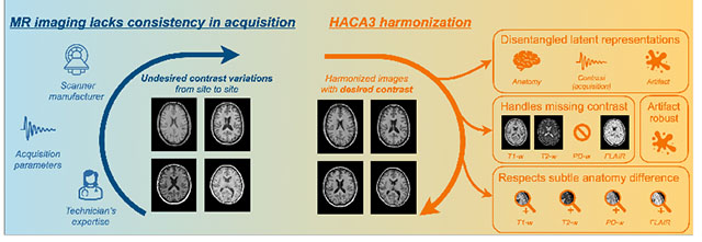
The lack of standardization and consistency of acquisition is a prominent issue in magnetic resonance (MR) imaging. This often causes undesired contrast variations in the acquired images due to differences in hardware and acquisition parameters. In recent years, image synthesis-based MR harmonization with disentanglement has been proposed to compensate for the undesired contrast variations. The general idea is to disentangle anatomy and contrast information from MR images to achieve cross-site harmonization. Despite the success of existing methods, we argue that major improvements can be made from three aspects. First, most existing methods are built upon the assumption that multi-contrast MR images of the same subject share the same anatomy. This assumption is questionable, since different MR contrasts are specialized to highlight different anatomical features. Second, these methods often require a fixed set of MR contrasts for training (e.g., both T1-weighted and T2-weighted images), limiting their applicability. Lastly, existing methods are generally sensitive to imaging artifacts. In this paper, we present Harmonization with Attention-based Contrast, Anatomy, and Artifact Awareness (HACA3), a novel approach to address these three issues. HACA3 incorporates an anatomy fusion module that accounts for the inherent anatomical differences between MR contrasts. Furthermore, HACA3 can be trained and applied to any combination of MR contrasts and is robust to imaging artifacts. HACA3 is developed and evaluated on diverse MR datasets acquired from 21 sites with varying field strengths, scanner platforms, and acquisition protocols. Experiments show that HACA3 achieves state-of-the-art harmonization performance under multiple image quality metrics. We also demonstrate the versatility and potential clinical impact of HACA3 on downstream tasks including white matter lesion segmentation on people with multiple sclerosis and longitudinal volumetric analyses for normal aging subjects. Code will be publicly available upon paper acceptance.

Graphical Abstract

1. Introduction

Magnetic resonance (MR) imaging is a widely used and flexible imaging modality for studying the human brain. By modifying underlying pulse sequences, multiple MR tissue contrasts can be acquired in a single imaging session, revealing different tissue properties and pathology (Prince and Links, 2006). For example, T₁-weighted (T₁-w) images typically show balanced soft tissue contrast between gray matter (GM) and white matter (WM). T₂-weighted (T₂-w) fluid-attenuated inversion recovery (FLAIR) images can detect WM lesions (Brown and et al., 2014). However, the flexibility of MR imaging also introduces drawbacks, most notably the lack of standardization and consistency between imaging studies. Changes in pulse sequences, imaging parameters, and scanner manufacturers often cause undesired contrast variations in acquired images. These contrast variations are frequently observed in multi-site and longitudinal studies, where acquiring images with identical protocols and platforms is challenging. It has been shown that directly processing these images without compensating for contrast variations can lead to biased and inconsistent measurements, also known as the domain shift problem (Biberacher et al., 2016; He et al., 2020; Zuo et al., 2021b).

Efforts from various aspects have been made to mitigate domain shift caused by inconsistent MR acquisition.

One approach is to standardize acquisition, such as the CMSC 2021 MRI guideline for multiple sclerosis (MS) study (Wattjes et al., 2021), which recommends core MR sequences for clinical practice. However, compliance with this guideline is not optimal, and even for sites following this guideline, manufacturers and protocols can still vary significantly across sites (Clark et al., 2022; Dewey et al., 2021). Another approach is statistical image harmonization, which focuses on a specific measurement, such as volumetric measurements, and uses statistical models to mitigate the effect of batches and sites (Beer et al., 2020; Fortin et al., 2018; Johnson et al., 2007; Newlin et al., 2023). However, a downside of statistical harmonization methods is that they often rely on specific assumptions about the statistical properties of the images being harmonized. These assumptions may not hold true for all imaging modalities or for all types of data (Cetin-Karayumak et al., 2020; Hu et al., 2023). Additionally, statistical methods may not be effective at harmonizing images with large differences in image quality or contrast, as they are designed to adjust for batch effects rather than address the underlying imaging artifacts (Dewey et al., 2019; Zuo et al., 2021b).

Harmonization through image synthesis is an emerging technique to alleviate domain shift.

In recent years, image synthesis-based MR harmonization techniques (Beizaee et al., 2023; Dewey et al., 2019, 2022; Gebre et al., 2023; Liu et al., 2021; Zuo et al., 2021a,b, 2022) have emerged to mitigate the lack of standardization in MR imaging. These methods are a special type of image-to-image translation (I2I) (Huang et al., 2018; Park et al., 2020; Liu et al., 2023; Roy et al., 2013; Zhu et al., 2017; Zuo et al., 2020), where the source and target images $x$ and $y$ come from different sites, such as two different T₁-w images from separate sites. In this context, we assume that images acquired with the same hardware and software come from the same (imaging) site. These harmonization methods learn a function, $f(\cdot )$, that translates $x$ from a source site to a target site, i.e., $\hat{y}=f(x)$ while preserving the underlying anatomy. Depending on the required training data, existing harmonization methods can be categorized into supervised and unsupervised methods. Supervised harmonization methods (Dewey et al., 2019; Tian et al., 2022) require a sample population to be imaged at multiple sites. The acquired images across sites (i.e., inter-site paired data), as shown in Fig. 1(a), are then used to train $f(\cdot )$. Although supervised harmonization generally exhibits superior performance due to the explicit voxel-level supervision provided by the inter-site paired data, its utility is limited to sites visited by traveling subjects. Conversely, unsupervised harmonization methods do not require inter-site paired data, thereby offering broader applicability. Most existing unsupervised methods for natural image I2I, such as CycleGAN (Zhu et al., 2017), UNIT (Liu et al., 2017), MUNIT (Huang et al., 2018), and CUT (Park et al., 2020) can be used to achieve unsupervised harmonization by translating MR images across imaging sites, as shown in Fig. 1(b). Even though cycle-consistency loss (assuming an identity transformation after a forward and a backward I2I) is typically used in these methods to encourage the preservation of anatomical features during I2I, geometry shift remains a significant issue due to the absence of direct supervision on anatomy across sites. Recent studies have shown that the cycle-consistency constraint is insufficient for unsupervised I2I in medical imaging (Gebre et al., 2023; Yang et al., 2018; Zuo et al., 2021b).

Figure 1:

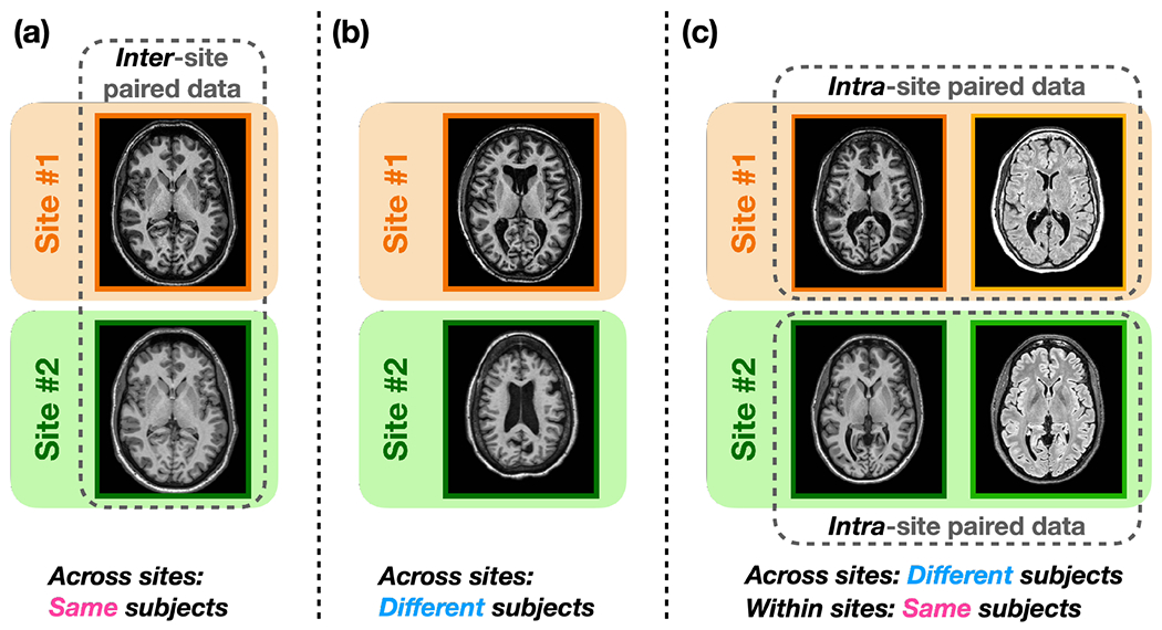
Training data required of the three types of harmonization methods. (a) Supervised harmonization methods (Dewey et al., 2019; Tian et al., 2022) require a sample group of subjects to be imaged across sites (i.e., inter-site paired data) for training. (b) Unsupervised methods developed for natural image I2I (Huang et al., 2018; Liu et al., 2018; Park et al., 2020; Zhu et al., 2017) can be trained with different subjects across sites. (c) Unsupervised harmonization methods with disentanglement (Ouyang et al., 2021; Zuo et al., 2021a,b) utilize the routinely acquired intra-site paired data for training.

A unique aspect of MR imaging motivates better unsupervised harmonization.

A distinctive feature of MR imaging is the routine acquisition of multi-contrast images of the same subject within a single imaging session (i.e., intra-site paired data) to highlight different anatomical properties. For example, the publicly available IXI (Biomedical Image Analysis Group, 2007) dataset includes T₁-w, T₂-w, and proton density-weighted (PD-w) images from different imaging sites. The OASIS3 (LaMontagne et al., 2019) dataset has intra-site paired T₁-w and T₂-w images. In recent years, unsupervised harmonization methods with disentanglement have been proposed to utilize intra-site paired data for improved harmonization. Figure 1(c) illustrates the training data used by these methods, where multi-contrast images of the same subject within each imaging site are employed. The core concept is to learn disentangled representations of anatomy and contrast (i.e., acquisition related) using intra-site paired images during training, so that the anatomy information and a desired contrast can be recombined at test time to achieve inter-site harmonization. For instance, Zuo et al. (2021a,b) disentangled anatomical and contrast information given intra-site paired T₁-w and T₂-w images. In their work, disentanglement was achieved with adversarial training and a similarity loss, assuming that the intra-site paired images share the same anatomical information. Ouyang et al. (2021) learned disentangled anatomy and contrast representations based on intra-site paired data with a margin hinge loss. The authors reported superior performance over existing unsupervised I2I methods such as CycleGAN (Zhu et al., 2017), due to supervision in geometry provided by the intra-site paired data.

However, current unsupervised harmonization methods miss an important consideration.

Most disentangling methods assume that intra-site paired images share identical underlying anatomy while only differing in image contrast (Chartsias et al., 2019; Dewey et al., 2020; Liu et al., 2022; Zuo et al., 2021a,b). This assumption is commonly used as an inductive bias, which is fundamental to learn disentanglement, according to Locatello et al. (2019). However, an overlooked aspect is that different MR contrasts are specifically designed to better reveal different tissue types and pathologies, which implies that the commonly used assumption of identical anatomy is not strictly accurate in MR imaging. For example, the images in Fig. 2 show that, although the two images come from the same subject, different MR contrasts reveal slightly different anatomical information. Specifically, the T₁-w image shows better contrast between GM, WM, and cerebrospinal fluid (highlighted by the green box), while the FLAIR image shows clearer boundaries for the WM lesions (highlighted by the orange circles). In this sense, these intra-site paired data are not perfect due to inherent anatomical differences between contrasts in MR imaging. Recent work by Träuble et al. (2021) have both theoretically and practically identified trade-offs between disentanglement and the quality of synthetic images when using imperfect paired data during training. Follow-up works in the medical domain by Ouyang et al. (2021) and Zuo et al. (2022) have reported on the negative impact of enforcing identical anatomies of intra-site paired data during image synthesis.

Figure 2:

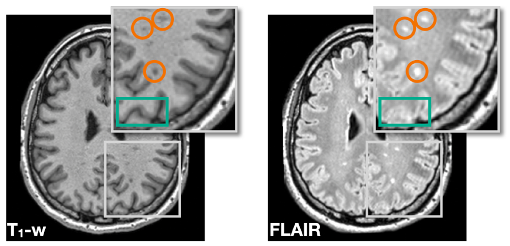
T₁-w and FLAIR images of a MS subject reveal slightly different anatomical features. The T₁-w image shows better contrast between GM, WM, and cerebrospinal fluid (highlighted by the green box), while the FLAIR image shows clearer boundaries for the WM lesions (highlighted by the orange circles).

Several unresolved problems persist with training a harmonization model that respects the anatomical differences between MR images with different acquisitions. First, the observable anatomy of intra-site paired images should be considered different, necessitating a new inductive bias to achieve disentanglement. Second, given different MR contrasts from the source site, the choice of source images has an impact on harmonization. Ideally, the model should choose an appropriate combination of contrasts to produce better harmonization. Third, imaging artifacts and missing contrasts should be handled to improve robustness and applicability.

In this paper, we propose harmonization with attention-based contrast, anatomy, and artifact awareness (HACA3), a novel harmonization approach to address these three issues. The contributions of the paper are as follows:

• We challenge the common assumption of identical anatomy for MR disentanglement and propose a new inductive bias to learn disentanglement from MR images. As a result, HACA3 respects the inherent anatomy difference between MR contrasts.

• We design a novel contrast and artifact attention mechanism to produce an optimal harmonized image based on the contrast and artifact information of each input image.

• HACA3 can be trained and applied to any set of MR contrasts by using a special design to handle missing contrasts.

HACA3 outperforms existing harmonization and I2I methods according to multiple image quality metrics. We use diverse MR datasets to demonstrate the broad applicability of HACA3 in downstream tasks including WM lesion segmentation and longitudinal volumetric analyses.

2. Methods

2.1. General framework

HACA3 follows an “encoder–attention–decoder” structure. In constrast to existing frameworks that disentangle anatomy and contrast (Dewey et al., 2020; Liu et al., 2022; Ouyang et al., 2021; Zuo et al., 2021b), HACA3 has an additional encoder—the artifact encoder—to assess the extent of artifacts present in the input MR images. Additionally, we introduce an attention module that analyzes the learned representations of contrast, anatomy, and artifacts to inform the decoder for better harmonization. Figure 3 shows the schematic framework of HACA3, which comprises three major components: 1) encoding, 2) anatomy fusion with attention, and 3) decoding. In this section, we provide an overview of HACA3’s general ideas. We offer detailed explanations of the encoding and attention components in Secs. 2.2 and 2.3, respectively. Implementation details, including network architectures and training losses, are described in Secs. 2.4 and 2.5.

Figure 3:

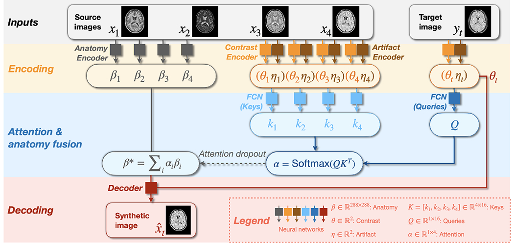
Schematic framework of HACA3. Networks with the same color share weights. Synthetic image ${\hat{x}}_t$ has the same contrast as the target image $y_t$ while preserving the anatomy from source images. Networks to process keys and queries are both fully connected networks (FCNs).

During training, HACA3 encodes the intra-site T₁-w, T₂-w, PD-w, and FLAIR images ($x_1,x_2,x_3,\text{and}{x}_4$, respectively) of the same subject into anatomy representations $\beta$, contrast representations $\theta$, and artifact representations $\eta$ using three corresponding encoders $E_{\beta }(\cdot ),E_{\theta }(\cdot )$, and $E_{\eta }(\cdot )$, respectively. Note that HACA3 does not require all four contrasts for training; it can be trained with any combination of MR tissue contrasts, as we describe in Sec. 2.3. Contrast and artifact representations (${\theta }_t$ and ${\eta }_t$) of the target image $y_t$ are also calculated during encoding. Following Chartsias et al. (2019); Dewey et al. (2020); Ouyang et al. (2021); Zuo et al. (2021a, 2022), HACA3 conducts intra-site I2I (e.g., intra-site T₁-w to T₂-w synthesis) with disentangled representations $\theta$ and $\beta$ during training. At test time, $\theta$ and $\beta$ from different sites are recombined to achieve inter-site harmonization. The anatomy representation $\beta$ has the same spatial dimension as images $x$ with five distinct intensity levels, calculated from a five-channel one-hot encoded map using Gumbel softmax Jang et al. (2017). This choice of anatomy representation has been explored and validated in multiple disentangling works (Chartsias et al., 2019; Dewey et al., 2020; Liu et al., 2020; Zuo et al., 2021b, 2022). The contrast representation $\theta$ and artifact representation $\eta$ are two-dimensional variables (i.e., $\theta ,\eta \in {ℝ}^2$). HACA3 then employs an attention module (we describe in Sec. 2.3) to process the learned representations $\theta$ and $\eta$ of both source and target images and find the optimal anatomy representation ${\beta }^{\mathrm{*}}$ for harmonization. The decoder subsequently recombines ${\beta }^{\mathrm{*}}$ and ${\theta }_t$ to generate a harmonized image ${\hat{x}}_t$ with the desired contrast as $y_t$ while preserving the anatomy from the source images. Since ${\eta }_t$ is processed by the attention module to calculate ${\beta }^{\mathrm{*}}$, it is not directly used by the decoder as input.

2.2. Encoding: contrast, anatomy, and artifacts

2.2.1. A new inductive bias to disentangle anatomy and contrast

We introduce a novel way to disentangle anatomy and contrast while respecting the natural anatomy differences between MR contrasts. The core concept of our anatomy encoder is based on contrastive learning (Park et al., 2020), which learns discriminative features from query, positive, and negative examples. Here, the query, positive, and negative examples are small image patches denoted as $p_q,p_{+}$, and $p_{-}$, respectively. As shown in Fig. 4, intra-site paired images of different MR contrasts are individually processed by the anatomy encoder to learn anatomical representations, where $i,j\in \{\mathrm{1,2},\mathrm{3,4}\}(i\ne j)$ are randomly selected contrasts. The query patch, $p_q$, is selected at a random location of ${\beta }_i$, i.e., the anatomical representation of contrast $i$. The positive patch $p_{+}$ is selected at the corresponding locations of ${\beta }_j$, where $j\ne i$. Negative patches $p_{-}^{(n)}$ are sampled at the same locations as $p_q$ from the original MR images as well as random locations from the learned $\beta$’s. Previous works (Chartsias et al., 2019; Dewey et al., 2020; Liu et al., 2022; Zuo et al., 2021a,b) have attempted to enforce identical anatomical representations between different MR contrasts. In other words, the query patch $p_q$ equals to the positive patch $p_{+}$ at every location. However, as we discussed in Sec. 1, this assumption is not entirely true. In our work, instead of enforcing $p_q$ to be identical to $p_{+}$, we encourage $p_q$ to be more similar to $p_{+}$ than to the $p_{-}^{(n)}$’s using the following loss function (Park et al., 2020)

$${ℒ}_{\text{C}}(p_q,p_{+},p_{-}^{(n)})=-\text{log}\left[\frac{\text{exp}(p_q\cdot p_{+})}{\text{exp}(p_q\cdot p_{+})+\frac{1}{N}{\sum }_{n=1}^N\text{exp}(p_q\cdot p_{-}^{(n)})}\right].$$ (1)

Figure 4:

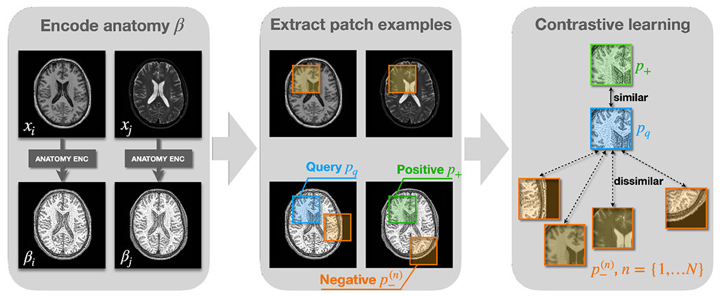
Learning anatomical representations $\beta$ with contrastive learning. $p_q,p_{+}$, and $p_{-}^{(n)}$ are query patch, positive patch, and negative patches, respectively. In previous works, $p_q$ is encouraged to be equal to $p_{+}$. In our work, $p_q$ is encouraged to be more similar to $p_{+}$ than to $p_{-}^{(n)}$ using Eq. 1, where $n=\{1,\dots ,N\}$ and $N$ is the number of negative patches.

Our inductive bias for disentanglement is that no matter how similar $p_q$ and $p_{-}^{(n)}$’s are, the positive patches $p_{+}$ should always be more similar to $p_q$, but not necessarily identical. The intuition is that $p_q$ and $p_{+}$ are representations of the same subject, while $p_{-}^{(n)}$’s either represent different anatomical information or the same subject with weighted contrasts. Choosing $p_{-}^{(n)}$’s from different locations of $\beta$’s ensures that the anatomical representations $\beta$ capture distinctive anatomical features at different locations, while choosing $p_{-}^{(n)}$ from original MR images of the same location encourages contrast information to be removed from $\beta$. Because our decoder takes both $\beta$ and $\theta$ as direct inputs to generate a harmonized image during training, contrast information is pushed to the $\theta$ branch, which we adopt from Zuo et al. (2021b).

2.2.2. Learning representations of artifacts

Our artifact encoder $E_{\eta }(\cdot )$ is designed to capture imaging artifacts that commonly occur in MR images and can negatively affect harmonization performance. By learning artifact representations $\eta$ from source MR images $x$, i.e., $\eta =E_{\eta }(x)$, the harmonization model is informed to avoid using images with high levels of artifacts. $E_{\eta }(\cdot )$, based on (Zuo et al., 2023), is also trained with contrastive learning, with query, positive, and negative examples being MR image slices denoted as $x_q,x_{+}$, and $x_{-}^{(m)}$, respectively. We prepare $x_q$ and $x_{+}$ by selecting 2D image slices from the same 3D MR volume, assuming they have similar levels of artifact. Negative examples $x_{-}^{(m)}$ are prepared in two ways: 1) by augmenting $x_q$ with simulated artifacts, such as motion and noise, and 2) by selecting 2D image slices from different volumes than $x_q$. In both cases, we assume $x_{-}^{(m)}$’s and $x_q$ have different levels of artifact. Since both simulated and real MR images are used as negative examples, $E(\eta )$ after training captures various artifacts beyond just motion and noise, as we demonstrated in our previous work Zuo et al. (2023). As shown in Fig. 5, query, positive, and negative images are processed by our artifact encoder $E_{\eta }(\cdot )$ to calculate the corresponding artifact representations $\eta$. The final loss to train $E_{\eta }(\cdot )$ is given by the contrastive loss ${ℒ}_{\mathrm{C}}\left({\eta }_q,{\eta }_{+},{\eta }_{-}^{(m)}\right)$ in Eq. 1, where $m=\{1,\dots ,M\}$ and $M$ is the total number of negative example images.

Figure 5:

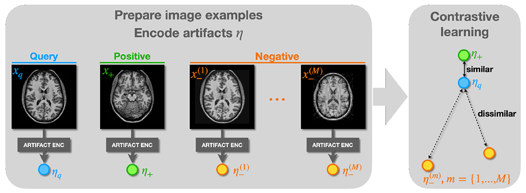
Learning artifact representations $\eta \in {ℝ}^2$ with contrastive learning. $x_q$ and $x_{+}$ are assumed to have the same level of artifacts, while $x_q$ and $x_{-}^{(m)}$ have different levels of artifacts. The contrastive loss is applied to encourage $\eta$ to preserve this relationship.

2.3. Decoding with attention

Given that ${\beta }_i$’s $(i=\{1,2,3,4\})$ from different images of the same subject should be similar but not necessarily identical, the choice of ${\beta }_i$ during decoding is crucial for successful harmonization. When harmonizing an MR contrast from a target site, it is intuitive to choose $\beta$ of the same contrast from the source site since similar pulse sequences usually reveal similar underlying anatomical information. However, this approach may not always be optimal when dealing with imaging artifacts and poor image quality. Alternatively, one can calculate $\beta$’s from all the available contrasts of the source images, which provides increased robustness against imaging artifacts and poor image quality. Previous works (Chartsias et al., 2019; Ouyang et al., 2021; Zuo et al., 2021a) have used either of the two ways separately, but HACA3 takes a step further by combining the advantages of both methods. Specifically, we propose a novel attention mechanism that takes both contrast and artifact into consideration when fusing anatomy from multiple source images. To do so, we use fully connected networks (FCNs) to learn keys $K=\left[k_1,k_2,k_3,k_4\right]$ and queries $Q$ (Vaswani et al., 2017), from the encoded $\theta$ and $\eta$ of both source and target images, as shown in Fig. 3. We then obtain attentions $\alpha \in {ℝ}^4$ by measuring the similarity between $K$ and $Q$ (Vaswani et al., 2017). The learned attentions highlight source images with similar contrast and image quality as the target image $y_t$ and guide the decoder to use the corresponding $\beta$’s for harmonization. Here, we assume that the target image $y_t$ has good image quality. The optimal anatomical representation, ${\beta }^{\mathrm{*}}$, is then obtained by conducting a weighted average with attention, i.e., ${\beta }^{\mathrm{*}}={\sum }_{i=1}^4{\alpha }_i{\beta }_i$, where ${\alpha }_i$ is the $i$-th dimension of $\alpha$. Finally, the decoder combines both ${\beta }^{\mathrm{*}}$ and ${\theta }_t$ to generate a synthetic image ${\hat{x}}_t$.

To enable HACA3 to handle an arbitrary number of MR contrasts during training, we introduce an attention dropout mechanism. When there are missing contrasts during training, the corresponding ${\alpha }_i$ is set to zero and the remaining ${\alpha }_i$’s are renormalized. This ensures that ${\sum }_{i=1}^4{\alpha }_i=1$ and $\beta$ of the missing contrasts will not be selected while calculating ${\beta }^{\mathrm{*}}$. Even when all four contrasts are available during training, one or more of the ${\alpha }_i$’s still have a chance to be randomly dropped out (set to zero), and the remaining ${\alpha }_i$’s are renormalized accordingly. During application, HACA3 handles missing contrasts in source images in a similar manner by setting the corresponding ${\alpha }_i$ to zero.

2.4. Network architectures

Network architectures are shown in Fig. 6. Our anatomy encoder and decoder are both U-Nets (Ronneberger et al., 2015) with four downsampling layers. The decoder has double the channels of the anatomy encoder, because we believe it needs larger network capacity to generate various MR contrasts. The contrast encoder is a fully convolutional network with four “Convolution–InstanceNorm–LeakyReLU” modules. The first convolutional kernel of our contrast encoder has a large kernel size. Because we believe contrast information of an MR image should be relatively global, using a large convolutional kernel to reduce the spatial dimension can help the model capture contrast information. Our artifact encoder has a DenseNet structure with four convolutional layers adopted from Zuo et al. (2023).

Figure 6:

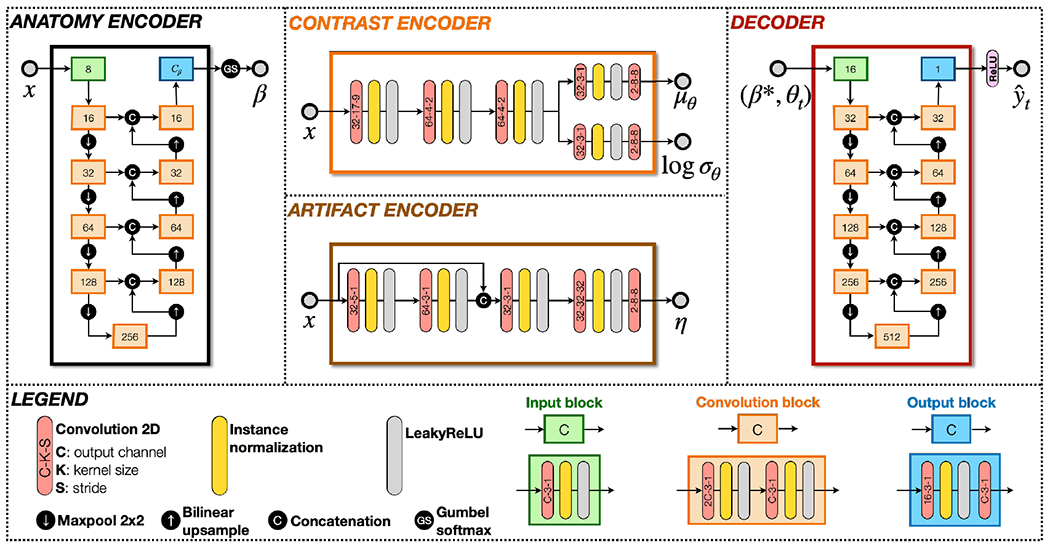
Network architectures of HACA3. The anatomy encoder and decoder are both U-Nets.

2.5. Implementation details and loss functions

The framework of HACA3 is a conditional variational autoencoder (CVAE). $\theta$ is the CVAE latent variable, and ${\beta }^{\mathrm{*}}$ is the condition. The CVAE loss to train HACA3 is given by

$${ℒ}_{\text{CVAE}}={|{\widehat{x}}_t-y_t|}_1+{\lambda }_1{𝒟}_{\text{KL}}[p(\theta \mid y_t)\left|\right|p(\theta )],$$ (2)

where ${𝒟}_{\mathrm{K}\mathrm{L}}$ is the KL divergence and $p(\theta )$ is a standard normal distribution, similar as most CVAE works. To further regularize HACA3, the synthetic image $\hat{x}$ is reanalyzed by the encoders $E_{\theta }(\cdot )$ and $E_{\eta }(\cdot )$ and a cycle consistency loss is calculated, i.e., ${ℒ}_{\text{cyc}}={\left|E_{\theta }\left({\hat{x}}_t\right)-{\theta }_t\right|}_1+{\left|E_{\eta }\left({\hat{x}}_t\right)-{\eta }_t\right|}_1$. The overall loss to train HACA3 includes ${ℒ}_{\mathrm{C}\mathrm{V}\mathrm{A}\mathrm{E}}$, contrastive losses for anatomy and artifact encoders (see Eq. 1), and ${ℒ}_{\text{cyc}}$, i.e.,

$${ℒ}_{\text{total}}={ℒ}_{\text{CVAE}}+{\lambda }_2{ℒ}_{\text{C}}(p_q,p_{+},p_{-}^{(n)})+{\lambda }_3{ℒ}_{\text{C}}({\eta }_q,{\eta }_{+},{\eta }_{-}^{(m)})+{\lambda }_4{ℒ}_{\text{cyc}},$$ (3)

where $\lambda$’s are hyperparameters. In our implementation, ${\lambda }_1$ through ${\lambda }_4$ are 10⁻⁵, 0.1, 0.1, and 0.1, respectively, which were chosen from the following reasons. Except for the KL divergence loss, the other loss terms have approximately equal magnitude after weighting by the $\lambda$’s. The $\mathrm{K}\mathrm{L}$ divergence loss is lightly penalized in training, because previous works (Higgins et al., 2017) have reported that when the KL divergence loss in a VAE model is heavily weighted, synthetic images tend to be blurry. We also want to keep the KL divergence term, since this allows HACA3 to generate MR images with various contrasts by sampling $\theta$ space. Dropping the KL divergence term will make HACA3 a conditional autoencoder, thus losing the ability to do variational sampling.

During training, target image $y_t$ is first randomly selected from intra-site paired images $x_1$ to $x_4$. In this case, HACA3 is trained to conduct intra-site I2I with disentanglement. We also select $y_t$ from a different site than the source images during training. In this case, only ${ℒ}_{\text{cyc}}$ is calculated to train the attention module with inter-site I2I. Our code will be publicly available upon paper acceptance.

3. Experiments and Results

3.1. Datasets and preprocessing

As we show in Table 1, HACA3 is developed and evaluated with highly variable MR datasets acquired from 21 sites, including healthy subjects (Sites S₁ to S₁₀) and people with MS (Sites S₁₁ to S₂₁). Out of the 21 sites we used in our training and evaluation, sites S₁₃ to S₂₁ are clinical centers and have more variability in image acquisition parameters. For these sites, a small percentage of images acquired from the same site may have different acquisition parameters, leading to different image contrasts.

Table 1.

MR images acquired from 21 sites were used to train and evaluate HACA3. Out of the 21 sites, 11 are publicly available (Biomedical Image Analysis Group, 2007; LaMontagne et al., 2019; Resnick et al., 2000; Carass et al., 2017). Magnetic field strengths are reported in teslas.

Site ID	S 1	S 2	S 3	S 4	S 5	S 6	S 7	S 8	S 9	S 10	S 11	S 12	S 13	S 14	S 15	S 16	S 17	S 18	S 19	S 20	S 21
Open data	✓	✓	✓	✓	✓	✓	✓	✓	✓	✓	✓	✕	✕	✕	✕	✕	✕	✕	✕	✕	✕
Manufacturer	Philips	Philips	Siemens	Siemens	Siemens	Siemens	Philips	Philips	Philips	Philips	Philips	Philips	Siemens	GE	Siemens	GE	Philips	Siemens	Siemens	Siemens	Siemens
Field	1.5	3.0	3.0	3.0	3.0	1.5	1.5	3.0	3.0	3.0	3.0	3.0	3.0	1.5	3.0	3.0	3.0	3.0	3.0	1.5	3.0
Population	Healthy	Healthy	Healthy	Healthy	Healthy	Healthy	Healthy	Healthy	Healthy	Healthy	MS	MS	MS	MS	MS	MS	MS	MS	MS	MS	MS
T1-w	✓	✓	✓	✓	✓	✓	✓	✓	✓	✓	✓	✓	✓	✓	✓	✓	✓	✓	✓	✓	✓
T2-w	✓	✓	✓	✓	✓	✓	✓	✓	✓	✓	✓	✓	✓	✓	✓	✓	✓	✓	✓	✓	✓
PD-w	✓	✓	✕	✕	✕	✕	✓	✓	✓	✓	✓	✓	✓	✕	✓	✕	✓	✕	✓	✕	✓
FLAIR	✕	✕	✕	✕	✕	✕	✓	✓	✓	✓	✓	✓	✓	✓	✓	✕	✓	✓	✓	✓	✓

All images were preprocessed with inhomogeneity correction (Tustison et al., 2010), super-resolution for 2D acquired images (Zhao et al., 2019, 2020), registration to an MNI atlas with $0.8{\mathrm{m}\mathrm{m}}^3$ resolution, and a WM peak normalization (Reinhold et al., 2019). For each site, ten training and two validation subjects were selected, each with two to four MR contrasts depending on availability. HACA3 was trained with 2D axial, coronal, and sagittal slices extracted from each 3D MR volume. We adopt the model introduced in Zuo et al. (2021b) to combine multi-orientation 2D slices into a 3D volume as our final harmonization result. Specifically, we use a 3D convolutional network that takes stacked 2D slices from axial, coronal, and sagittal orientations as input and generates a final 3D volume as output.

3.2. Exploring the latent contrast, anatomy, and artifact space

The contrast encoder $E_{\theta }(\cdot )$ in HACA3 captures acquisition-related information from MR images. After training, we expect the learned representations in $\theta$ space to reflect information about site and MR contrasts . Figure 7(a) shows the learned contrast space of T₁-w, T₂-w, PD-w, and FLAIR images from ten representative sites. Each point in the plot corresponds to a 3D MR volume, and the $\theta$ value of each MR volume is calculated by averaging the $\theta$’s of the center 20 axial slices per volume. The results demonstrate that the four MR contrasts are separated in $\theta$ space. Furthermore, we observe that the $\theta$ values of PD-w and T₂-w images are located next to each other, which is consistent with the fact that these two contrasts are often acquired simultaneously with different echo times.

Figure 7:

Contrast representations $\theta$ of 10 representative sites. (a) $\theta$’s of T₁-w, T₂-w, PD-w, and FLAIR images. (b) $\theta$’s of T₁-w images from different sites. Circled numbers show $\theta$ values of six representative images. Corresponding MR images are shown in (c).

To investigate the impact of sites on the learned $\theta$ values, we plotted the $\theta$ values of T₁-w images from the ten sites in Fig. 7(b). The results reveal several interesting observations. First, the $\theta$ values of images from the same site are generally closer to each other than those from different sites. Second, images with overlapping $\theta$ clusters share similar echo time, inversion time, and image contrast, as demonstrated in cases ④ and ⑤ of Figs. 7(b) and (c). Third, we observed several outliers with $\theta$ values deviating from their main clusters, as showcased by ① and ② of Fig. 7(b). Upon examination, we discovered that case ② is a post-gadolinium T₁-w (post T₁-w) image that had erroneous header information identifying it as a pre-gadolinium T₁-w (pre T₁-w). This error is evident from inspection of ② in Fig.7(c). With respect to case ③, the image was acquired using different parameters than the other images from Site S₁₂.

Figure 8 shows the learned anatomical representations $\beta$ of intra-site paired T₁-w, T₂-w, PD-w, and FLAIR images. Generally, $\beta$’s of the four images are visually similar, suggesting that they capture similar anatomical information. However, there are subtle differences highlighted by the orange boxes, indicating that each MR contrast reveals slightly different anatomical information. This observation supports our motivation behind developing HACA3—that different MR contrasts reveal slightly different anatomical information.

Figure 8:

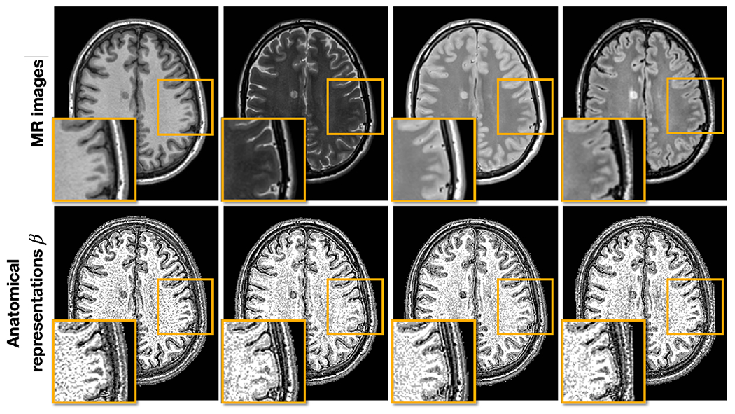
Anatomical representations $\beta$ of intra-site paired data. The top row shows T₁-w, T₂-w, PD-w, and FLAIR images, respectively, with the inset being a zoomed up version of the orange box. The bottom row shows the corresponding $\beta$’s of each contrast and the same zoomed in region.

In our previous work (Zuo et al., 2023), we demonstrated that the artifact encoder captures various cases of poor quality images. However, it is also crucial to ensure that our attention mechanism works properly in highlighting similar contrast source images and downplaying the role of poor quality source images. To investigate this, we present three harmonization scenarios where T₁-w, T₂-w, PD-w, and FLAIR images from Sites S₁₃ or S₁₇ are harmonized to a FLAIR image from Site S₁₂—i.e., Sites S₁₃ or S₁₇ are the source and Site S₁₂ is the target. Figure 9(a) shows the scenario where all four source modalities have good image quality, resulting in most of the attention (77%) being on the FLAIR image of the source site S₁₃—see the attention column in Fig. 9. This makes sense since the attention $\alpha$ is computed from representations of contrast and artifacts and then used to select the corresponding anatomical representation $\beta$ during harmonization. Figure 9(b) depicts another harmonization scenario where the FLAIR image from the source site S₁₇ has higher noise levels. Here, the attention on the source FLAIR image has decreased, while the other three MR contrasts have increased. The attention model seeks anatomical information from other contrasts to compensate for the lower quality of the source FLAIR. As a result, the harmonized FLAIR image has a better quality appearance while preserving anatomical details such as the WM lesions. Figure 9(c) presents an extreme scenario in which the source FLAIR image has even higher noise levels and motion artifacts. In this case, the attention $\alpha$ on the source FLAIR image further decreases to seek alternative anatomical information from other contrasts. As a result, the harmonized FLAIR image demonstrates improved image quality and anatomical fidelity. It is important to note that the decrease in attention from Figs. 9(b) to (c) is likely due to differences in image quality rather than contrast, as the images in Figs. 9(b) and (c) come from the same source site.

Figure 9:

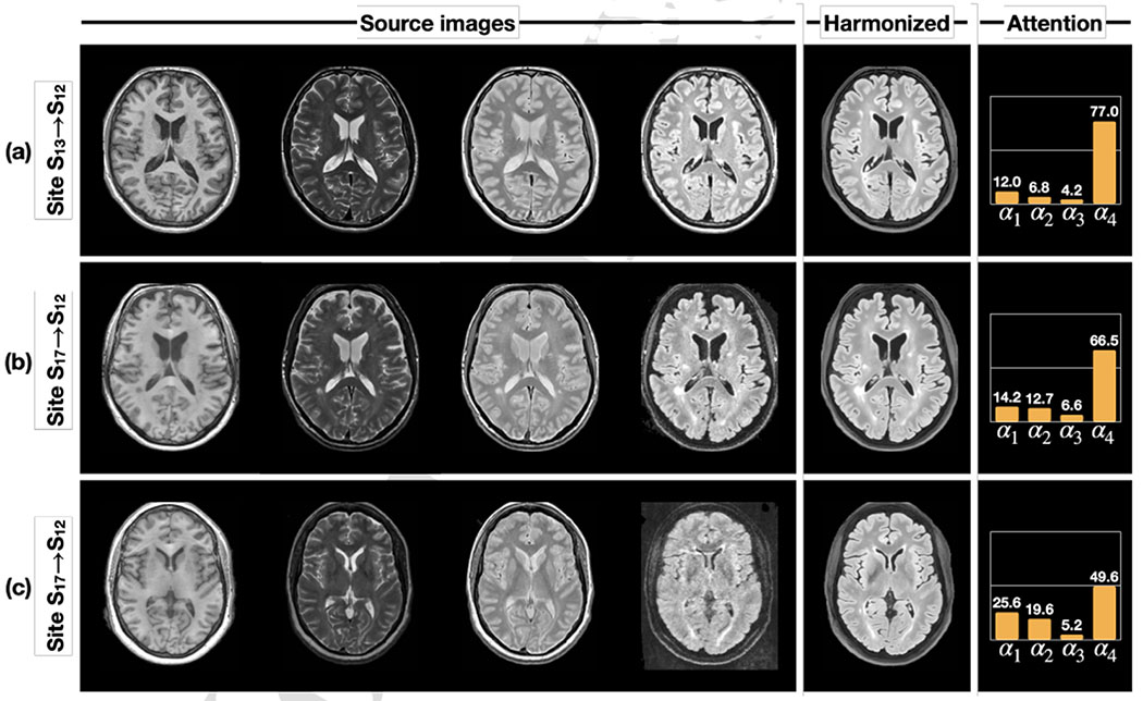
The learned attention $\alpha$ changes with three different harmonization scenarios. In all three scenarios, T₁-w, T₂-w, PD-w, and FLAIR images from sites (S₁₃ or S₁₇) are harmonized to a FLAIR image of a different site—S₁₂ in this case.

3.3. Numerical comparisons of multi-site MR image harmonization

3.3.1. Comparing with supervised and unsupervised harmonization methods

In this experiment, we seek a harmonization model that translates T₁-w images from a source site to a target site. We used a held-out dataset with 12 subjects traveling across Sites S₁₁ (source) and S₁₂ (target) to quantitatively evaluate HACA3 and other methods. The same traveling dataset was also used in Dewey et al. (2019) for evaluation. These methods come from three broad types: 1) unsupervised I2I including CycleGAN (Zhu et al., 2017) and CUT (Park et al., 2020), 2) two unsupervised harmonization methods based on intra-site paired data (Adeli et al., 2021; Zuo et al., 2021b), and 3) supervised harmonization (Dewey et al., 2019). Structural similarity index (SSIM) (Wang et al., 2004) and peak signal-to-noise ratio (PSNR) are used to quantitatively evaluate all methods. Throughout the paper, both SSIM and PSNR are calculated on the MR image.

Comparison with unsupervised I2I with cycle consistency constraint in anatomy:

As shown in Fig. 10, we compared HACA3 (pink) with CycleGAN (green) and CUT (red). Both CycleGAN and CUT were trained on unpaired T₁-w images from Sites S₁₁ and S₁₂. HACA3 outperforms both methods with statistical significance (p < 0.01 in a paired Wilcoxon signed-rank test). Surprisingly, CycleGAN and CUT did not show much improvement compared to the unharmonized images (blue), even though the synthetic images are visually fine, as shown in Fig. 10. We hypothesize that this may be due to the issue of geometry shift, as indicated by the orange arrows in Fig. 10. This observation supports the findings in previous studies (Gebre et al., 2023; Yang et al., 2018) that the cycle consistency constraint for anatomy alone is not sufficient for MR harmonization.

Figure 10:

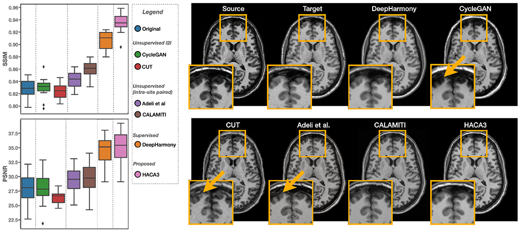
Numerical comparisons between HACA3 (proposed) and other methods using a held-out dataset of inter-site traveling subjects. SSIM and PSNR of T₁-w images are calculated. Example T₁-w images are shown on the right.

Comparison with unsupervised harmonization based-on intra-site paired data:

We then compared HACA3 to existing unsupervised harmonization methods that are also based on intra-site paired data, including Adeli et al. (Adeli et al., 2021) and CALAMITI (Zuo et al., 2021b). Both methods were trained on intra-site paired T₁-w and T₂-w images with disentanglement. As shown in Fig. 10(a), HACA3 (pink) outperforms these methods (purple and brown) with statistical significance (p < 0.01 in a paired Wilcoxon signed-rank test). Given that all three methods are based on intra-site paired images for training, we believe that the superior performance of HACA3 comes from its ability to use multiple MR contrasts during application. In Sec. 3.3.2, we further explore the impact of this ability with various cases of input MR contrasts. Interestingly, all three methods have better performance than unsupervised I2I methods, which demonstrates the benefits of using intra-site paired data in harmonization.

Comparison with supervised harmonization:

Given that HACA3 can be trained on a wide variety of data, we finally ask ourselves whether it could potentially outperform supervised harmonization methods. To test this hypothesis, we compared HACA3 with DeepHarmony (Dewey et al., 2019), a supervised harmonization method that was specifically trained on inter-site paired images from S₁₁ and S₁₂. The same evaluation dataset as Dewey et al. (2019) was used here to evaluate HACA3 and other comparison methods. A paired Wilcoxon signed rank test shows that HACA3 outperforms DeepHarmony (orange) in SSIM (see Fig. 10) with statistical significance (p < 0.01). This result highlights the potential of HACA3 as a versatile and effective harmonization method.

3.3.2. Ablation: HACA3 handling missing contrasts

HACA3 is designed to handle any number of source MR contrasts during both training and application. To investigate this ability and the impact of each source contrast on the final harmonization result, we conducted an ablation study on all possible scenarios during application. Specifically, we used the same inter-site traveling dataset as Sec. 3.3.1 in our ablation study ($N=12$ subjects traveled between Sites S₁₁ and S₁₂ with T₁-w, T₂-w, PD-w, and FLAIR images). We then applied HACA3 to harmonize images from S₁₁ to S₁₂ and reported the SSIM values between the harmonized image and the real S₁₂ image for each of T₁-w, T₂-w, PD-w, and FLAIR being the target contrast. Results in Figs. 11(a)–(d) demonstrate HACA3’s robust performance across various combinations of input contrasts. The best performance is typically achieved when all four contrasts are used as input, however, the results are similar when only two or three input contrasts are used as input. For our target contrasts of T₁-w, T₂-w, and FLAIR, we observed that missing the corresponding source image often has an negative impact on the harmonization results. However, when PD-w is the target contrast, the performance deviates from this pattern. In this case, missing PD-w as the source image actually improves the results. We hypothesize that this is due, in part, to the generally lower resolutions of PD-w and T₂-w images. Lastly, when FLAIR is the target contrast, the harmonization performance is lower compared to the other target contrasts. This can be attributed to the challenges in reproducing WM lesions, which are harder to replicate accurately. HACA3 heavily relies on information from T₁-w and FLAIR images to achieve this task. Overall, our study highlights the robustness of HACA3 in handling various input contrasts and sheds light on the factors influencing its performance.

Figure 11:

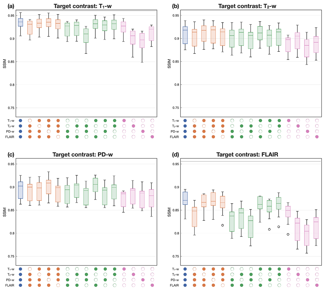
HACA3 handling different availability of source images. From (a) to (d): target image being T₁-w, T₂-w, PD-w, and FLAIR images, respectively. Colored boxplots represent different numbers of source images. The panel below the boxplots indicates which images were used as input to the harmonization (with an empty circle indicating the absence of a particular contrast).

3.4. Evaluating HACA3 in downstream tasks

To validate HACA3’s ability to alleviate domain shift, we showcase two different downstream image analysis tasks: 1) WM lesion segmentation and 2) whole brain parcellation. The first task is based on multi-site cross-sectional data and the second task focuses on longitudinal analyses with scanner change and upgrades.

3.4.1. WM lesion segmentation on multi-site data

As shown in Fig. 12(a), two MS datasets acquired from sites S₁₁ and S₁₂ were used in this experiment. The training data (S₁₂) for MS lesion segmentation include T₁-w (not shown), FLAIR, and expert delineations of WM lesions of 10 subjects. The testing data (S₁₁) to evaluate lesion segmentation come from ILLSC 2015 (Carass et al., 2017), which is publicly available. A 3D U-Net with four downsampling layers was trained with MR images and delineations from S₁₂ using a Dice similarity coefficient (DSC) loss.

Figure 12:

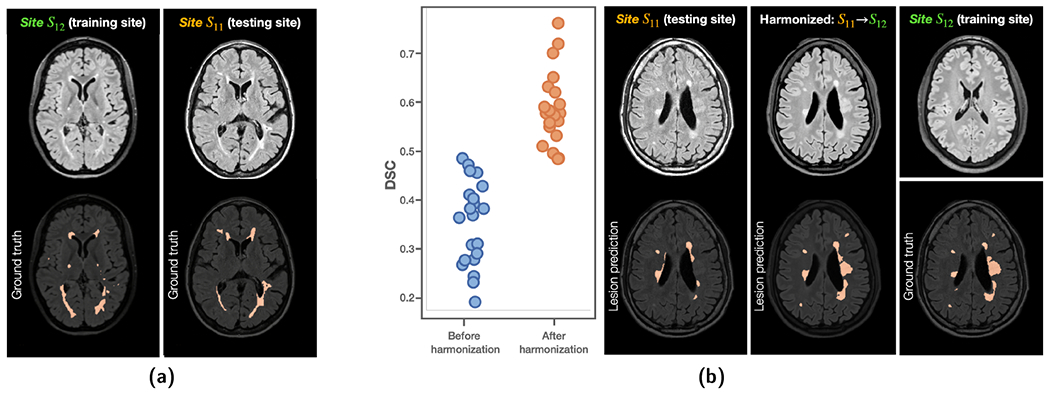
(a) Training and testing sites for WM lesion segmentation with a 3D U-Net. (b) DSC showed improvements after harmonizing images from the testing site (Site S₁₁) to the lesion training site (Site S₁₂). Example images are shown on the right.

The 3D U-Net achieved a DSC of 0.593 ± 0.072 (similar to the best results reported in Tohidi et al. (2022) and close to the inter-rater variability of Carass et al. (2017)) in a five-fold cross validation on S₁₂, which it was trained on However, when the 3D U-Net was applied to S₁₁, the DSC dropped to 0.348 ± 0.089 due to domain shift. HACA3 was then applied to harmonize images from Site S₁₁ to S₁₂ aiming at alleviating domain shift, and the lesion segmentation was reevaluated. As shown in Fig. 12(b), DSC has improved to 0.590 ± 0.075, which is similar to the performance on the training site. It is worth noting that WM lesions are particularly difficult to synthesize and characterize due to the large variation in lesion size and location. It is encouraging that HACA3 generates high fidelity images that show effectiveness in WM lesion segmentation both qualitatively and quantitatively.

3.4.2. Whole brain parcellation on longitudinal data.

We used two public longitudinal datasets, i.e., OASIS3 (Sites S₃ to S₆) (LaMontagne et al., 2019) and BLSA (Sites S₇ to S₁₀) (Resnick et al., 2000), to evaluate HACA3 for longitudinal analyses. The number of subjects and sessions of each dataset is shown in Table 2. The same preprocessing was applied here, followed by a whole brain parcellation on T₁-w images using Huo et al. (2019). For the cortical GM (cGM), cerebral WM (WM), and lateral ventricles (LatV), a structure-specific linear mixed effects (LME) model $y_{ij}=a_0+a_1{x}_{ij}+b_j+{ϵ}_{ij}$ was fitted, where $x_{ij}$ and $y_{ij}$ are age and percentage structural volume (structural volume divided by total brain volume) of session $i$ and subject $j$, respectively. We reuse the notations $x,y,i$, and $j$ to be consistent with the LME literature (Erus et al., 2018). $b_j\sim 𝓝\left(0,{\sigma }_b^2\right)$ is the subject-specific bias, and ${\sigma }_b^2$ models population variance. ${ϵ}_{ij}\sim 𝓝\left(0,{\sigma }_{ϵ}^2\right)$ is the error term modeling noise in observations. Based on the LME, longitudinal intra-class correlations (ICCs) were calculated to characterize the effect of harmonization in longitudinal analysis with ICC defined by,

$$\text{ICC}=\frac{{\sigma }_b^2}{{\sigma }_b^2+{\sigma }_{ϵ}^2}\times 100\text{\%},$$

where an ICC close to 0% means the noise in observations is the dominant factor over population difference. An ICC close to 100% indicates most variances are due to the natural population difference rather than noisy observations. Assuming the effect of scanner change and upgrades are alleviated with harmonization, we would expect increased ICCs after harmonization. Table 2 shows that the ICCs and ${\sigma }_{ϵ}^2$ of all structures from both datasets were improved after harmonization.

Table 2.

Longitudinal ICCs and ${\sigma }_{ϵ}^2$ of cGM, WM, and LatV before and after harmonization. Details about each dataset are shown in Table 1 (Sites S₃ to S₁₀). For longitudinal ICC higher values are better, while for ${\sigma }_{ϵ}^2$ lower values are better.

Dataset	# Subjects	# Sessions	Structure	ICC (%) ↑		${\sigma }_{ϵ}^2$ ↓
				Before	After	Before	After
OASIS3	721	1,117	cGM	81.95	95.13	83.6	44.8
			WM	83.54	95.85	64.1	31.9
			LatV	96.37	96.38	25.4	25.2
BLSA	1,037	2,655	cGM	86.98	96.49	106.9	52.1
			WM	87.35	96.38	133.1	59.3
			LatV	95.96	95.99	46.2	29.7

4. Discussion and Conclusion

In this paper, we present HACA3, a novel harmonization approach with attention-based contrast, anatomy, and artifact awareness. We demonstrate the effectiveness of HACA3 through extensive experiments and evaluations on diverse MR datasets. HACA3 learns a disentangled latent space of contrast and anatomy, allowing different MR contrasts and imaging sites to be differentiated in the contrast space $\theta$. This demonstrates HACA3’s capability to capture complex information about image acquisition and contrast, which is crucial for contrast-accurate MR image harmonization. Moreover, we show that the anatomical representations $\beta$ of intra-site paired images, while generally similar, reveal slight different anatomical features. This finding is consistent with HACA3’s design, which respects the inherent anatomical differences between MR contrasts. HACA3’s capability to understand these nuanced anatomical features is essential for generating harmonized images with high anatomical fidelity. The learned artifact representations $\eta$ not only inform HACA3 for robust harmonization but also provide rich information for MR quality control, as we have demonstrated in previous work (Zuo et al., 2023). Our attention mechanism based on $\eta$ and $\theta$ identifies poor quality images at the source site and learns to dynamically combine anatomical information.

By respecting contrast and artifacts, HACA3 produces harmonized images that are high quality and suitable for downstream image analyses. Numerical comparisons show that HACA3 significantly outperforms unsupervised I2I methods, unsupervised harmonization methods based on intra-site paired images, and a supervised harmonization method. We have also explored the impact of different source image availability on harmonization results, demonstrating HACA3’s robustness under varying input conditions.

Our study highlights the potential clinical impact of HACA3 through two different downstream tasks. In the WM lesion segmentation task, HACA3 provides high-quality synthetic FLAIR images with preserved lesion structure. We demonstrate improved lesion segmentation performance by alleviating domain shift. Accurate lesion detection is essential for making informed treatment decisions in MS. Specifically, clinicians may recommend stronger immune therapies if harmonization helps identify lesions that are otherwise missed by the lesion segmentation algorithm. Conversely, if harmonization helps correct false lesions, clinicians may not recommend changing or escalating therapies unnecessarily. For the longitudinal volumetric analysis task, HACA3 promotes consistent longitudinal volumetric analyses in terms of longitudinal ICCs and error residual. This can facilitate more meaningful longitudinal analyses of the normal aging process of the human brain.

Despite its strengths, we discuss some limitations and intriguing findings that may motivate future research. First, the imbalance of available MR contrasts in training data may have a negative impact on harmonization performance. Specifically, if a contrast is missing in many training sites, HACA3 may not be sufficiently trained due to the lack of training data of that particular contrast. It is worth noting that this issue of imbalanced training data is not specific to HACA3, but is present in most deep learning methods. We believe this issue can be mitigated by importance sampling training data based on the prevalence of each contrast, so each MR contrast would appear equally during training. Second, HACA3 currently focuses on T₁-w, T₂-w, PD-w, and FLAIR images. While this covers a large range of MR contrasts in clinical applications, we believe HACA3’s capability is beyond that. As we show in Fig. 7, even though HACA3 was not trained on post T₁-w, the theta-encoder is still able to capture this difference in contrast. This capacity should be explored in future research for potential extension of HACA3 to include more MR contrasts and even other imaging modalities (e.g., computed tomography (Chartsias et al., 2019)). Third, each attention variable ${\alpha }_i$ is currently applied to the entire image with the $i$-th contrast, but these variables could be extended in the future to be spatially variable as well. By allowing the attention to vary across spatial locations, it can better adapt to the local anatomical features and provide more fine-grained control over the harmonization process. This could potentially lead to better performance, especially in areas with complex or subtle anatomical differences, depending on the source images and target contrasts.

In conclusion, our work on HACA3 showcases its ability to address challenges in MR image harmonization and its potential to improve the quality and consistency of neuroimaging studies. By successfully disentangling contrast and anatomy, respecting inherent anatomical differences, and leveraging attention mechanisms for handling artifacts, HACA3 sets a new benchmark in MR image harmonization and promises to advance the field of harmonization. Future research should focus on addressing the limitations and further expanding the applicability of HACA3 to a wider range of MR contrasts and imaging scenarios.

Highlights.

• A unified harmonization approach that disentangles contrast and anatomy, while respecting inherent anatomical difference between MR contrasts.

• A novel attention mechanism optimally processes anatomical information based on image contrast and artifacts.

• Extensive evaluations on 21 imaging sites with diverse acquisition parameters and image quality.

References

- Adeli E, et al. 2021. Representation learning with statistical independence to mitigate bias, in: Proceedings of the IEEE/CVF Winter Conference on Applications of Computer Vision, pp. 2513–2523. [DOI] [PMC free article] [PubMed] [Google Scholar]
- Beer JC, et al. 2020. Longitudinal ComBat: A method for harmonizing longitudinal multi-scanner imaging data. NeuroImage 220, 117129. [DOI] [PMC free article] [PubMed] [Google Scholar]
- Beizaee F, et al. 2023. Harmonizing flows: Unsupervised mr harmonization based on normalizing flows. arXiv preprint arXiv:2301.11551. [Google Scholar]
- Biberacher V, et al. 2016. Intra-and interscanner variability of magnetic resonance imaging based volumetry in multiple sclerosis. NeuroImage 142, 188–197. [DOI] [PubMed] [Google Scholar]
- Biomedical Image Analysis Group, 2007. IXI Brain Development Dataset. https://brain-development.org/ixi-dataset/.
- Brown RW, et al. 2014. Magnetic resonance imaging: physical principles and sequence design (Second edition.) Wiley. [Google Scholar]
- Carass A, et al. 2017. Longitudinal multiple sclerosis lesion segmentation data resource. Data in brief 12, 346–350. [DOI] [PMC free article] [PubMed] [Google Scholar]
- Cetin-Karayumak, et al. 2020. Exploring the limits of ComBat method for multi-site diffusion MRI harmonization. bioRxiv , 2020–11. [Google Scholar]
- Chartsias A, et al. 2019. Disentangled representation learning in cardiac image analysis. Medical Image Analysis 58, 101535. [DOI] [PMC free article] [PubMed] [Google Scholar]
- Clark KA, et al. 2022. Inter-scanner brain MRI volumetric biases persist even in a harmonized multi-subject study of multiple sclerosis. bioRxiv , 2022–05. [DOI] [PMC free article] [PubMed] [Google Scholar]
- Dewey BE, et al. 2019. DeepHarmony: a deep learning approach to contrast harmonization across scanner changes. Magnetic Resonance Imaging 64, 160–170. [DOI] [PMC free article] [PubMed] [Google Scholar]
- Dewey BE, et al. 2020. A disentangled latent space for cross-site MRI harmonization, in: International Conference on Medical Image Computing and Computer-Assisted Intervention, pp. 720–729. [Google Scholar]
- Dewey BE, et al. 2021. Improving the utilization of standardized MRIs in multiple sclerosis care: a pragmatic trial perspective, in: The consortium of multiple sclerosis centers. [Google Scholar]
- Dewey BE, et al. 2022. Chapter 11 - Medical image harmonization through synthesis, in: Biomedical Image Synthesis and Simulation. Academic Press. The MICCAI Society book Series, pp. 217–232. [Google Scholar]
- Erus G, et al. 2018. Longitudinally and inter-site consistent multi-atlas based parcellation of brain anatomy using harmonized atlases. NeuroImage 166, 71–78. [DOI] [PMC free article] [PubMed] [Google Scholar]
- Fortin JP, et al. 2018. Harmonization of cortical thickness measurements across scanners and sites. NeuroImage 167, 104–120. [DOI] [PMC free article] [PubMed] [Google Scholar]
- Gebre RK, et al. 2023. Cross–scanner harmonization methods for structural MRI may need further work: A comparison study. NeuroImage 269, 119912. [DOI] [PMC free article] [PubMed] [Google Scholar]
- He Y, et al. 2020. Self Domain Adapted Network, in: International Conference on Medical Image Computing and Computer-Assisted Intervention, pp. 437–446. [Google Scholar]
- Higgins I, et al. 2017. Beta-VAE: Learning basic visual concepts with a constrained variational framework, in: International conference on learning representations. [Google Scholar]
- Hu F, et al. 2023. Image harmonization: A review of statistical and deep learning methods for removing batch effects and evaluation metrics for effective harmonization. NeuroImage, 120125. [DOI] [PMC free article] [PubMed] [Google Scholar]
- Huang X, et al. 2018. Multimodal unsupervised image-to-image translation, in: Proceedings of the European Conference on Computer Vision, pp. 172–189. [Google Scholar]
- Huo Y, et al. 2019. 3D whole brain segmentation using spatially localized atlas network tiles. NeuroImage 194, 105–119. [DOI] [PMC free article] [PubMed] [Google Scholar]
- Jang E, et al. 2017. Categorical reparameterization with gumbel-softmax, in: International Conference on Learning Representations. [Google Scholar]
- Johnson WE, et al. 2007. Adjusting batch effects in microarray expression data using empirical bayes methods. Biostatistics 8, 118–127. [DOI] [PubMed] [Google Scholar]
- LaMontagne PJ, et al. 2019. OASIS-3: Longitudinal neuroimaging, clinical, and cognitive dataset for normal aging and Alzheimer disease. medRxiv. [Google Scholar]
- Liu AH, et al. 2018. A Unified Feature Disentangler for Multi-domain Image Translation and Manipulation, in: Advances in Neural Information Processing Systems, pp. 2590–2599. [Google Scholar]
- Liu J, et al. 2023. One model to synthesize them all: Multi-contrast multi-scale transformer for missing data imputation. IEEE Transactions on Medical Imaging. [DOI] [PMC free article] [PubMed] [Google Scholar]
- Liu M, et al. 2021. Style transfer using generative adversarial networks for multi-site MRI harmonization, in: International Conference on Medical Image Computing and Computer-Assisted Intervention, Springer. pp. 313–322. [DOI] [PMC free article] [PubMed] [Google Scholar]
- Liu MY, et al. 2017. Unsupervised Image-to-image Translation Networks, in: Advances in Neural Information Processing Systems, pp. 700–708. [Google Scholar]
- Liu Y, et al. 2020. Variational intensity cross channel encoder for unsupervised vessel segmentation on OCT angiography, in: Medical Imaging 2020: Image Processing, SPIE. pp. 206–212. [Google Scholar]
- Liu Y, et al. 2022. Disentangled representation learning for OCTA vessel segmentation with limited training data. IEEE Transactions on Medical Imaging. [DOI] [PMC free article] [PubMed] [Google Scholar]
- Locatello F, et al. 2019. Challenging common assumptions in the unsupervised learning of disentangled representations, in: International Conference on Machine Learning, PMLR. pp. 4114–4124. [Google Scholar]
- Newlin NR, et al. 2023. Comparing voxel-and feature-wise harmonization of complex graph measures from multiple sites for structural brain network investigation of aging, in: Medical Imaging 2023: Image Processing, SPIE. pp. 524–530. [DOI] [PMC free article] [PubMed] [Google Scholar]
- Ouyang J, et al. 2021. Representation disentanglement for multi-modal brain MRI analysis, in: International Conference on Information Processing in Medical Imaging, Springer. pp. 321–333. [DOI] [PMC free article] [PubMed] [Google Scholar]
- Park T, et al. 2020. Contrastive learning for unpaired image-to-image translation, in: European Conference on Computer Vision, Springer. pp. 319–345. [Google Scholar]
- Prince JL, Links JM, 2006. Medical imaging signals and systems. Pearson Prentice Hall Upper Saddle River. [Google Scholar]
- Reinhold JC, et al. 2019. Evaluating the impact of intensity normalization on MR image synthesis, in: Medical Imaging 2019: Image Processing, International Society for Optics and Photonics. p. 109493H. [DOI] [PMC free article] [PubMed] [Google Scholar]
- Resnick SM, et al. 2000. One-year age changes in mri brain volumes in older adults. Cerebral Cortex 10, 464–472. [DOI] [PubMed] [Google Scholar]
- Ronneberger O, et al. 2015. U-Net: convolutional networks for biomedical image segmentation, in: International Conference on Medical Image Computing and Computer-Assisted Intervention, pp. 234–241. [Google Scholar]
- Roy S, et al. 2013. Magnetic Resonance Image Example Based Contrast Synthesis. IEEE Trans. Med. Imag 32, 2348–2363. [DOI] [PMC free article] [PubMed] [Google Scholar]
- Tian D, et al. 2022. A deep learning-based multisite neuroimage harmonization framework established with a traveling-subject dataset. NeuroImage, 119297. [DOI] [PubMed] [Google Scholar]
- Tohidi P, et al. 2022. Multiple sclerosis brain lesion segmentation with different architecture ensembles, in: Medical Imaging 2022: Biomedical Applications in Molecular, Structural, and Functional Imaging, SPIE. pp. 578–585. [Google Scholar]
- Träuble F, et al. 2021. On disentangled representations learned from correlated data, in: International Conference on Machine Learning, PMLR. pp. 10401–10412. [Google Scholar]
- Tustison NJ, et al. 2010. N4ITK: improved N3 bias correction. IEEE Transactions on Medical Imaging 29, 1310–1320. [DOI] [PMC free article] [PubMed] [Google Scholar]
- Vaswani A, et al. 2017. Attention is all you need. Advances in Neural Information Processing Systems 30. [Google Scholar]
- Wang Z, et al. 2004. Image quality assessment: from error visibility to structural similarity. IEEE Transactions on Image Processing 13, 600–612. [DOI] [PubMed] [Google Scholar]
- Wattjes MP, et al. 2021. 2021 MAGNIMS–CMSC–NAIMS consensus recommendations on the use of MRI in patients with multiple sclerosis. The Lancet Neurology 20, 653–670. [DOI] [PubMed] [Google Scholar]
- Yang H, et al. 2018. Unpaired brain MR-to-CT synthesis using a structure-constrained cyclegan, in: Deep Learning in Medical Image Analysis and Multimodal Learning for Clinical Decision Support. Springer, pp. 174–182. [Google Scholar]
- Zhao C, et al. 2019. Applications of a deep learning method for anti-aliasing and super-resolution in MRI. Mag. Reson. Im 64, 132–141. [DOI] [PMC free article] [PubMed] [Google Scholar]
- Zhao C, et al. 2020. SMORE: a self-supervised anti-aliasing and super-resolution algorithm for MRI using deep learning. IEEE Transactions on Medical Imaging 40, 805–817. [DOI] [PMC free article] [PubMed] [Google Scholar]
- Zhu JY, et al. 2017. Unpaired image-to-image translation using cycle-consistent adversarial networks, in: Proceedings of the IEEE International Conference on Computer Vision, pp. 2223–2232. [Google Scholar]
- Zuo L, et al. 2020. Synthesizing realistic brain MR images with noise control, in: International Workshop on Simulation and Synthesis in Medical Imaging, pp. 21–31. [Google Scholar]
- Zuo L, et al. 2021a. Information-based disentangled representation learning for unsupervised MR harmonization, in: International Conference on Information Processing in Medical Imaging, Springer. pp. 346–359. [Google Scholar]
- Zuo L, et al. 2021b. Unsupervised MR harmonization by learning disentangled representations using information bottleneck theory. NeuroImage 243, 118569. [DOI] [PMC free article] [PubMed] [Google Scholar]
- Zuo L, et al. 2022. Disentangling a single MR modality, in: Data Augmentation, Labelling, and Imperfections, Springer Nature; Switzerland. pp. 54–63. [Google Scholar]
- Zuo L, et al. 2023. A latent space for unsupervised MR image quality control via artifact assessment, in: Medical Imaging 2023: Image Processing, SPIE. pp. 278–283. [Google Scholar]